
Abstract
The precision tools equipped with active vibration isolation platform in high-tech facilities are sensitive to low-frequency vibration. Currently, there are neither standards nor rules to select the time period of vibration data for conducting the spectral analysis of low-frequency vibration, and none of the analyses can be used to compare and discuss the differences of spectral amplitude generated by the selection of different time periods. Therefore, to estimate the amplitude of low-frequency vibration, the spectral analysis at low-frequency range is crucial. This paper is to elaborate the spectral analysis procedures on various band widths by using zero-padding on the vibration signal in low-frequency band. The mechanism not only facilitates to obtain more reliable result but also to lay a common base for comparison from different user. Finally, the in situ measurement data, including high-speed train-induced low-frequency vibration, are used to exemplify the length of time period affects the results of spectral analysis, either on narrowband or one-third octave band analysis.
Introduction
When conducting spectral analysis of digital signal, the mathematical operation of discrete Fourier transform (DFT) or the algorithm of fast Fourier transform (FFT) is widely used. One should select a finite length (or finite time period) of digital signal to conduct FFT, but there is neither standard nor rule to select the duration of time period (or frequency resolution, bandwidth) for conducting spectral analysis.
In general, most researchers select the time period for FFT using data point with a power of 2 (N = 2
r
), if the interval of equally spaced N samples is
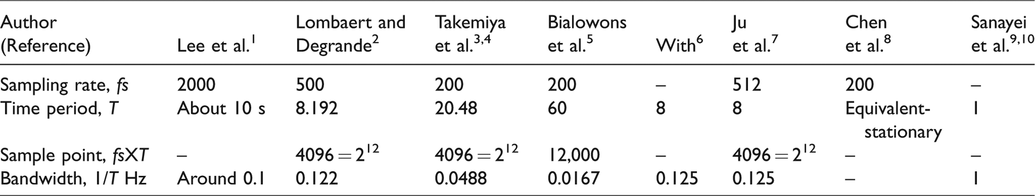
In spectral analysis of vibration signal, depends on the sampling rate, time period of the record may be different for analysis. For example, Lee et al. 1 studied micro-vibration evaluations on chip fabrication facilities by using 2000 Hz sampling rate, T is about 10 s results in around 0.1 Hz resolution, Lombaert and Degrande 2 validated a numerical prediction model for free field traffic induced vibrations by in situ experiments using 500 Hz sampling rate, T = 8.192 s, the equivalent resolution is 0.122 Hz, Takemiya et al. 3 and Takemiya 4 studied high-speed train on viaduct induced ground vibrations using 200 Hz sampling rate, T = 20.48 s, the corresponding resolution is 0.0488 Hz, Bialowons et al. 5 measured the ground motion in various sites using 200 Hz sampling rate and T = 60 s, With With and Bodare 6 looked into train-induced vibration inside buildings using T = 8 s, the resolution is 0.125 Hz, Ju et al. 7 studied characteristics of train-induced ground vibrations using 512 Hz sampling rate and T = 8 s, the resolution is 0.125 Hz, Chen et al. 8 dealt with the transient vibration by equivalent-stationary duration which means the duration between 5% and 95% of accumulated energy, Sanayei et al.9,10 measured and predicted train-induced vibration in building following FTA assessment manual 11 using T = 1 s, but the lowest one-third octave band frequency is 10 Hz in their studies, which does not meet the frequency range 1–80 Hz of VC curves. The parameters revealed in the papers are summarized in Table 1. Besides, there are many researches focus on the study and analysis of traffic-induced vibration through field test data.12–29 However, as the authors know, none of analyses be compared and discussed on the differences of amplitude in frequency domain generated by the selection of different time periods. Thus, the difference of amplitude may result in opposite conclusion of the vibration impact on the facilities, even though, it may get into controversial lawsuits/legal issues later.
The parameters revealed in different papers.
After years of study, the authors found out that the selection of the time periods or sample points for spectral analysis is critical because different selections may lead to different results especially for the low-frequency vibration. Nevertheless, so far, there is no experimental benchmark for reliable reference to choose the time periods/sample points.
Therefore, the purpose of this paper is to demonstrate a better mechanism for obtaining reliable results that could be comparable and communicable among domain researchers. In this paper, the generic vibration criteria (VC) and the theoretical background of spectral analysis will be provided. Then, in situ experiments include traffic-induced vibration and ambient vibration for exploring a better mechanism to select the proper time periods/sample points will be illustrated in detail. Finally, a conclusion and recommendation will be made.
Generic vibration criteria
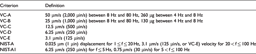
It is customary to use so-called generic VC when designing high-tech facilities and advance R&D labs. Eric Ungar and Colin Gordon29,30 developed the VC curves using one-third octave band in the early 1980s. With the evolution of the advanced semiconductor process to small feature size, many tools were equipped with active vibration system, the VC curves have been changed in order to avoid the problem of the amplification of low-frequency vibration. The frequency range below VC-C is modified from 8–80 Hz to 1–80 Hz and the amplitude is “flattened” as shown in Figure 1. The numerical definition of VC curves is listed in Table 2.
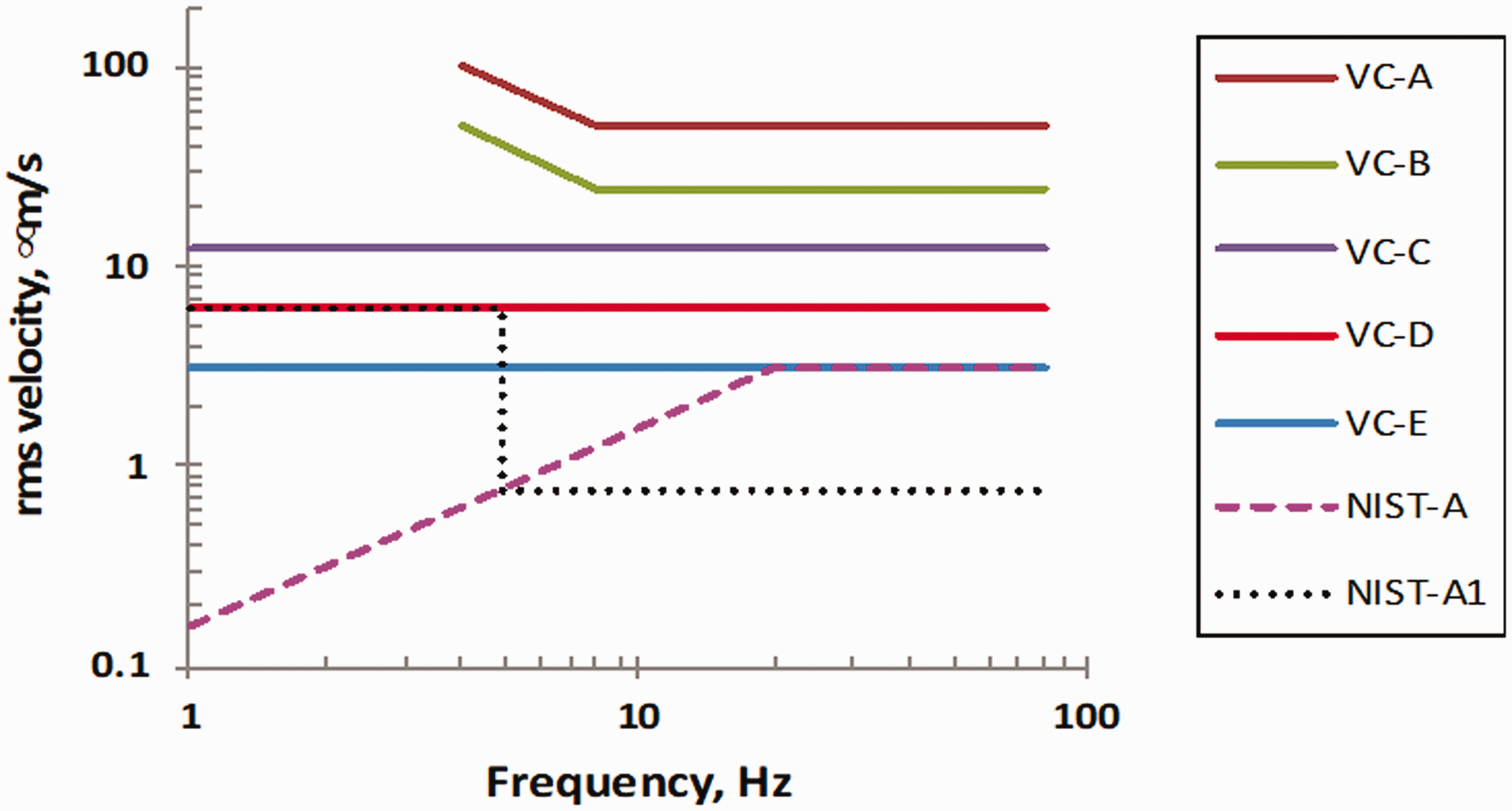
Vibration criteria curves.
Numerical definition of vibration criteria curves.
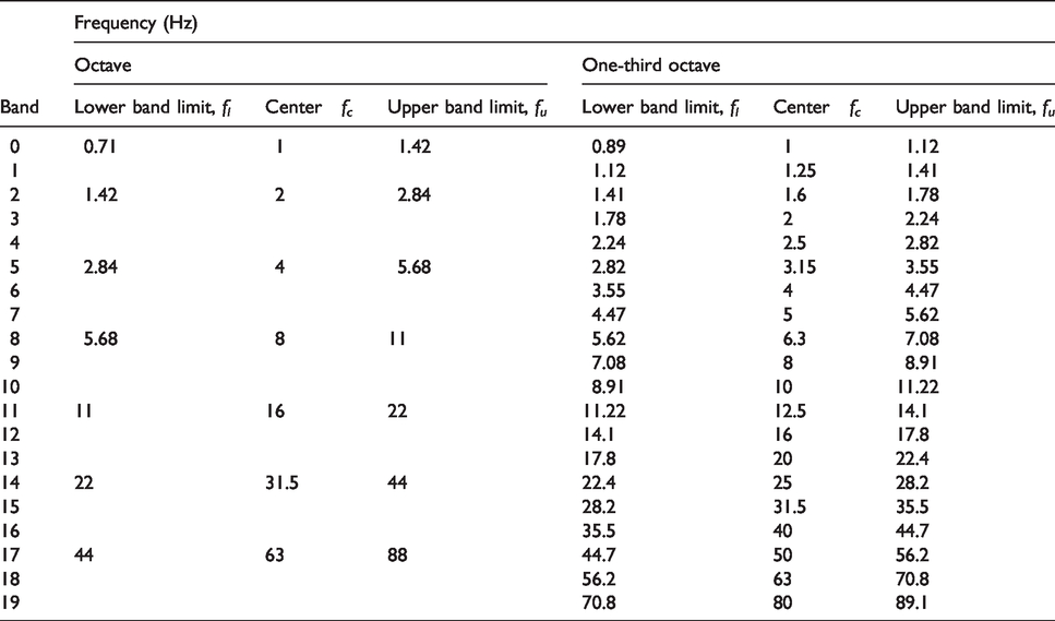
The VC curves are based on one-third octave band. An octave band is a frequency band where the highest frequency is twice the lowest frequency (i.e., 
Center and band limit frequency of octave and one-third octave band.
Spectral analysis of low-frequency (long period) signals
In this section, the procedures of spectral analysis on low-frequency signal will be discussed, which include fundamental definition of DFT, the effect of zero-padding on spectral analysis, and the calculation of one-third octave band.
Discrete–Time Fourier Transform and DFT
Consider a discrete–time of (t) is presented as x[n] which can be expressed as an impulse train in time domain
The Fourier transform of 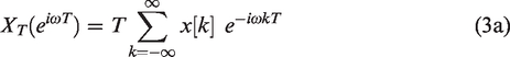
Since 
Note that the
Spectral analysis of signal with zero-padding
Zero-padding is an operation in which more zeros are appended to the tail of original sequence. For example, adding zeros to the tail of a sequence with N samples, then the total sample is N + number of zeros added, say M. This insight can be understood by increasing the frequency resolution through using zero-padding. Assume that a new signal is created by zero-padding x according to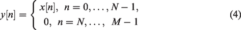
This indicated the augmentation of signal x with M − N zeros (of course M > N). Now, if the DFT of y[n] is applied, the implicit assumption indicated that it is periodic with period M. As more and more zeros are appended to the signal, the periodicity assumption will more and more resemble the assumption that the signal is zero outside the sampled range. Hence, by padding the signal with zeros one shift from the DFT assumption (periodicity) to the truncated DTFT assumption (that the signal is zero outside the known range). Consequently, the DFT of the signal will “move” toward the truncated DTFT.
Consider a time series, as shown below

(a) DFT of x[n]
With the same procedure of analysis, the result is also shown in Figure 2(b). It is observed that for case of DFT with 32 point of x[n], the peak of the Fourier amplitude cannot actually identify the dominant frequency of the signal, besides, the peak amplitude also shows lower than the other test cases. If zero padding is used, the exact dominant frequency under peak amplitude can be identified. It is concluded that padding zero to the end of signal can obtain a more stable Fourier spectrum.
Analysis of one-third octave band
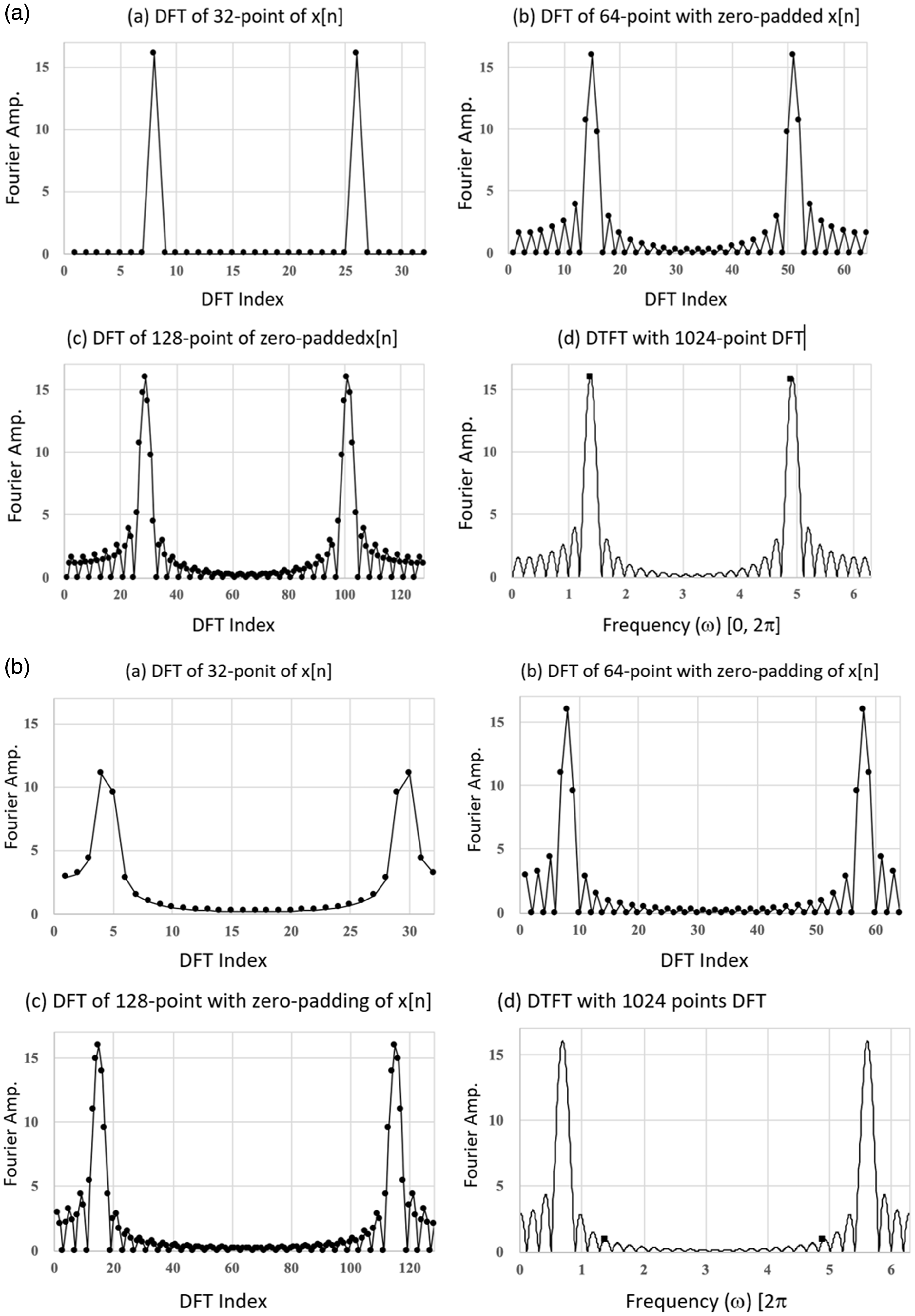
Since the amplitude of the long period vibration signal plays an important role on the quality control of the product in high-tech facilities, therefore, to develop a reasonable and well-acceptable estimation of the broadband spectrum is required. The procedures of the spectral analysis to estimate the square root of the mean square of a signal are briefly as follows: Transform time domain sequence Calculate one-sided auto-spectral density 3. Integrate 4. Calculate the square root of the mean square amplitude
where NT is the period, excluding zero-padded.
where 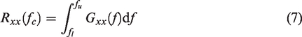

There are two issues raised in this spectral analysis: (1) What is adequate bandwidth? and (2) What is the adequate duration, NT, for transient data?
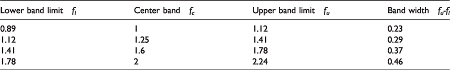
The band limit and bandwidth of one-third octave band below 2 Hz are shown in the Table 4 (based on equation (1)). It is observed that the bandwidth is less than 0.5 Hz when the center frequency is below 2 Hz, while the smallest bandwidth (
Band limit and band width of one-third octave band below 2 Hz.
At the early stage, the development of VC-curves only up to the lower frequency limit of 4 Hz, because the frequency resolution for lower frequency limit of 4 Hz is not important (bandwidth is wider for larger center frequency). But for the later evolution of VC curves, the frequency limit is lowered to 1 Hz, then the frequency resolution will affect the accuracy at low frequency range. In general, one chooses the duration of time period T based on the sampling rate of the data acquisition system, the major concern is
One could use a longer time period to get better frequency resolution since Use T = 4.0 s (total data point is 4 x 256 = 1024 points) and the bandwidth is Use zero-padded 4 s to the tail of original sequence (T = 8.0 s), the bandwidth is Use zero-padded 12 s, the bandwidth is
Figure 3 plots the discrete PSD with frequency axis less than 2 Hz. The center frequency of one-third octave band 1, 1.25, 1.6, and 2 Hz are also marked and their corresponding band limits 0.89, 1.12, 1.41, 1.78, and 2.24 Hz (one-third octave band) are plotted. To calculate the mean square amplitude (equation (8)) within the band limit (either at center frequency1.0 Hz or 1.25 Hz) using different length of signal, the mean square amplitude may have difference due to the effect of interpolation (as shown in Figure 3). For example, when the bandwidth is 0.25 Hz (T = 4 s), for case of center frequency 1 Hz (bandwidth: 0.89–1.12 Hz), to evaluate the PSD value under such band limit, the PSD value at 0.89 Hz needs to be interpolated between the values at 0.75 Hz and 1 Hz. In the case of 4 s + 4s zeros, the band limit 0.89 Hz and 1.12 Hz, and the frequency interval for such case is 0.875 Hz, and 1.125 Hz on the both sides of the frequency 1 Hz which shows very close to the band limit even through the interpolation is applied. From Figure 3, one can see that the mean square amplitude under the 1/3 octave band limit at center frequency 1 Hz and 1.25 Hz is obviously different if the data length used to calculate the PSD is different. If the signal frequency resolution is not consistent with the lower and upper bound frequency of one-third octave band, this may lead to significant differences in the calculation of mean square amplitude.
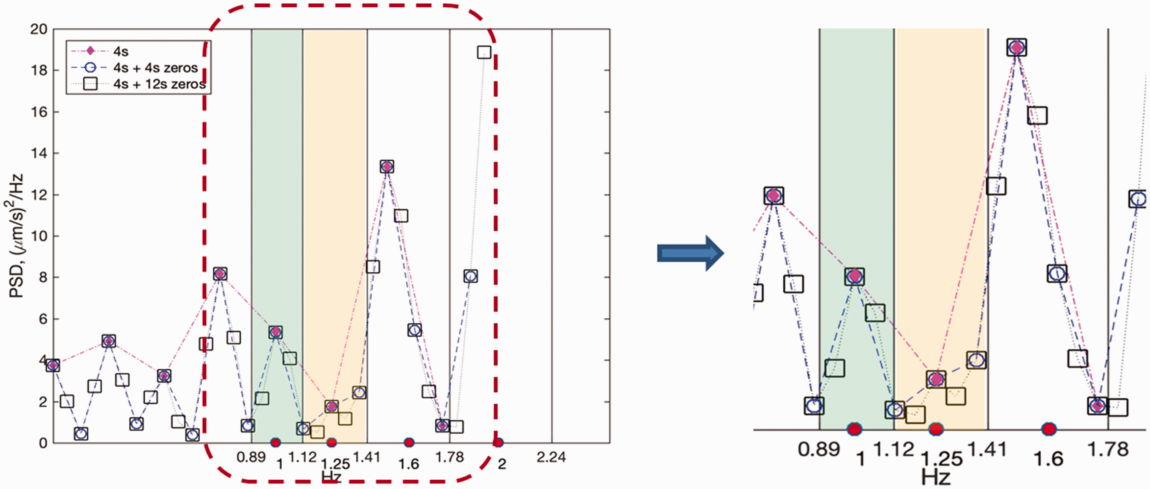
PSD of narrowband data with different bandwidth by zero-padding and compare with the band limit of one-third octave band less than 2 Hz.
Because the position of the band limit may not consistent with each discrete frequency band (due to different duration of signal). This phenomenon indicates that using different data length (with or without zero-padding), the plot of mean square amplitude may be different. This may cause some argument in the evaluation of impact of low-frequency vibration signal for high-tech facilities.
Results from in situ measurement data analysis
The in situ measurement data including ambient and transient vibration induced by high-speed train at free-field and at nearby building were taken as examples to compare the spectral analysis results of different methods.
1/3 Octave band analysis of high-speed train induced transient vibration at free field
Figure 4 shows a free-field time history example of high-speed train induced vibration, the distance between measurement location and the railway is 175 m and the measurement direction is along the railway. The high-speed railway structure is a simply supported viaduct structure with 30-m span length. To collect the data the frequency range of recorded time history is set as 100 Hz and the sampling rate is 256 Hz. The moving window technique with window length of 4 s and overlap 3.0 s was conducted. The interval of 4 s between 80 and 84 s of the recorded time history from one of the moving time windows was selected for spectral analysis. This interval includes the maximum amplitude of time history as shown with dash lines in Figure 4.
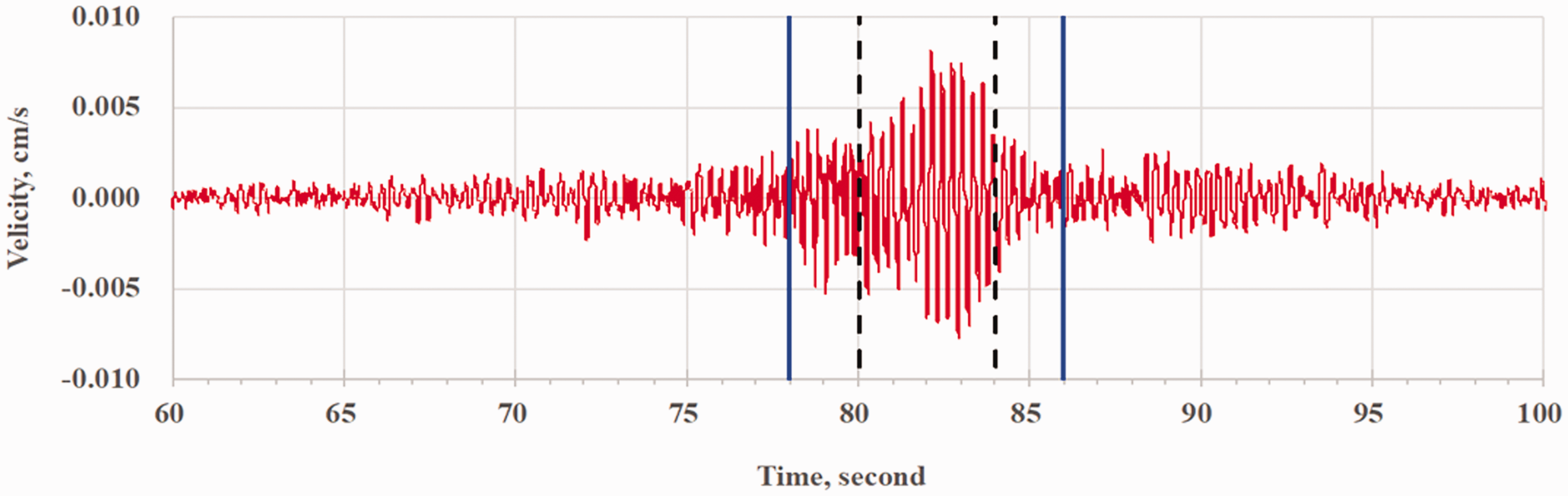
Free-field time history example of high-speed train induced vibration.
Three cases of analysis as mentioned in previous section are conducted. The maximum amplitude is at center frequency 3.15 Hz. Results from three different approaches (with and without zero-padding) to calculate the discrete PSD between 2 Hz and 3.75 Hz is shown in Figure 5. The distribution band limit of center frequency 3.15 Hz between 2.82 Hz and 3.55 Hz is also shown (1/3 octave band). It is observed that the maximum value of PSD is almost the same by using the data set with time period of 4 s + 4 s zero-padding with frequency resolution
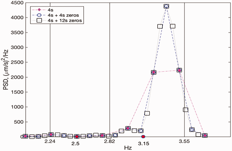
PSD of narrowband data with different bandwidth by zero-padding and compare with the band limit of one-third octave band at 3.15 Hz.
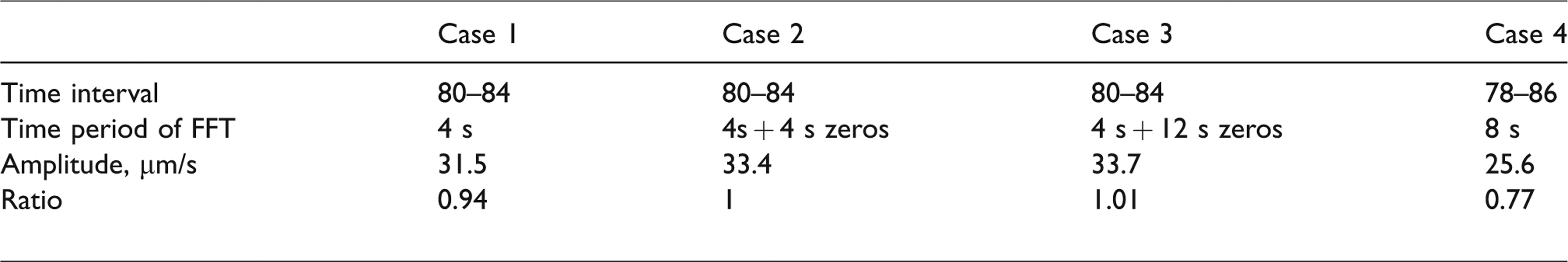
The mean value of the area (as shown in equation (7)) under the discrete PSD enclosed by the 1/3 octave band limit at each center frequency of 3.15 Hz is calculated. Figure 6(a) to (d) shows the area of four test cases, Figure 6(a) to (c) is the aforementioned cases, Figure 6(d) is an additional case that the interval of 78–86 s of the time history was taken (the time duration is 8 s with bandwidth of 0.125 Hz), as shown at blue dot line in Figure 4. It is observed that the analysis of a transient signal with and without zero padding, the amplitude of PSD is very different. The root-mean square amplitude according to equation (8) of four cases is shown in Table 5. The ratio of Case 1, Case 3, and Case 4 to Case 2 are 0.94, 1.01, and 0.77, respectively.
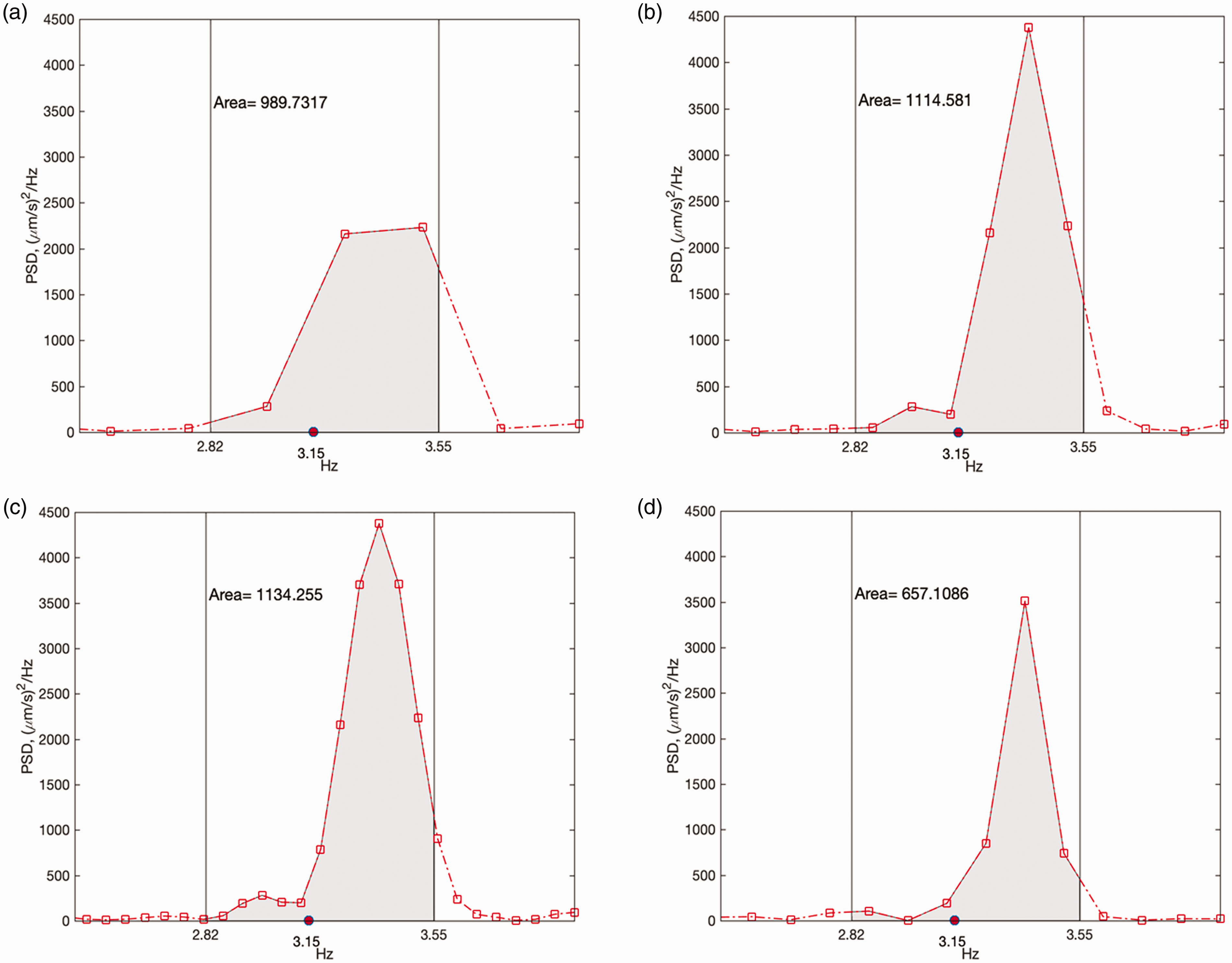
Area of discrete PSD curve enclosed by band limit of center frequency 3.15 Hz, (a) 4 s, 1024 points, (b) 4 s + 4s zeros, 2048 points, (c) 4 s + 12s zeros, 4096 points, and (d) 8 s, 2048 points.
The one-third octave band amplitude at center frequency 3.15 Hz.
For a finite length time signal 
For stationary signal, it has been proved that the power spectral density
As shown in Figure 6(a) to (c), frequency resolution (duration of data) plays a significant role on the estimation of signal PSD. Therefore, it is important to reveal the user-defined parameters in the signal analysis, especially the spectral amplitude which is very crucial to make decision on the amplitude level. Based on this case study, one can find that the cases of Cases 2 and 3 with zero-padded data, one can have almost the same results. Regarding the impact on high-tech facility due to train-induced vibration, the estimated spectral amplitude by using different duration of data collected from the field may have different results. As shown in Table 5, one can see the amplitude of Case 1 (4 s) is 31.5 µm/s which is 23% larger than Case 4 (8 s) 25.6 µm/s. The difference is quite significant so the comparison from different analyzer may show different result. It is necessary to define a physical-base analytical method on the estimation of PSD.
Narrowband analysis of high-speed train-induced transient vibration at free field
To conduct narrowband analysis, the procedures are basically the same as broadband analysis (one-third octave band). First, the band limit difference,
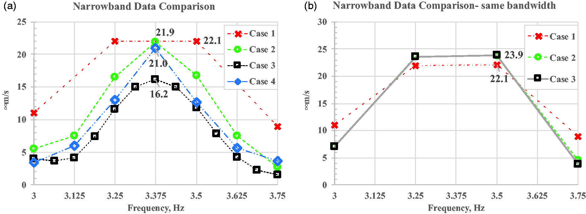
The narrowband amplitude between 3 Hz and 3.75 Hz, (a) the narrowband amplitude of four cases and (b) case 2 and 3 convert to 0.25 Hz bandwidth.
The bandwidth from Case 1 to Case 4 is 0.25 Hz, 0.125 Hz, 0.0625 Hz, and 0.125 Hz, respectively.
From Figure 7(a) it is observed that: The bandwidth 0.25 Hz (using data length of 4 s) is too rough to catch the frequency where the peak value occurred. In order to compare the narrowband amplitude, the comparison should have the same bandwidth. Otherwise, the narrower bandwidth (Case 3, narrowest bandwidth 0.0625 Hz) normally results in smaller amplitude (Case 3, smallest amplitude 16.2 µm/s). Compare the amplitude of Case 2 (4 s + 4 s zeros) and Case 4 (8 s) that have the same bandwidth (0.125 Hz), and it shows again the shorter time period leads to larger amplitude.
One can also confirm that the sequence of data with/without zero-padding also satisfy Parseval’s Theorem. The Parseval’s Theorem in discrete form can be written as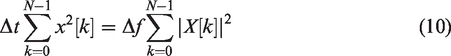
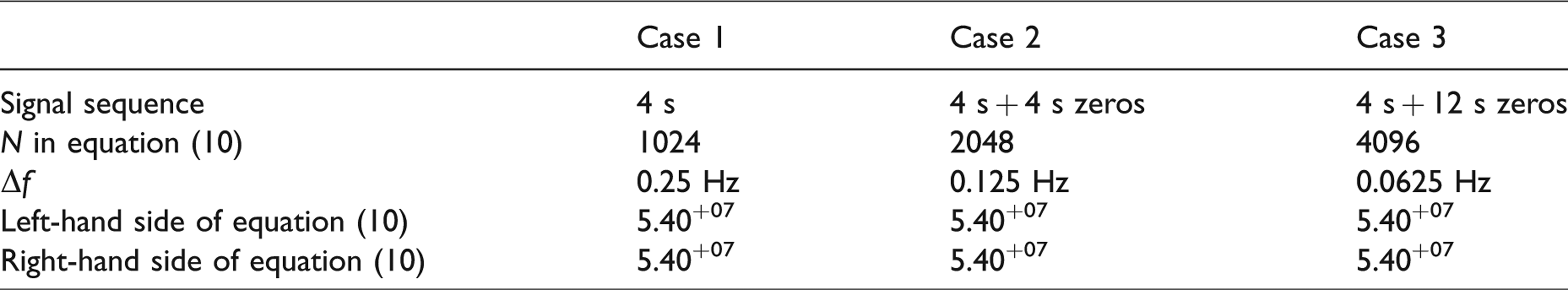
The Parseval’s Theorem can be regarded as energy conservation in the time domain and frequency domain. Then, one can further check if the sequences with/without zero-pad satisfy Parseval’s Theorem. The left-hand and right-hand side of equation (10) are summarized in Table 6, it is obvious that no matter how many zeros padded to original sequence, the left-hand side remains unchanged; and the right-hand side of equation (10) in the frequency domain, in spite of different N and
The results of Parseval’s theorem in discrete form.
However, one can utilize dense narrowband data to get coarse narrowband amplitude: Take Case 1 to Case 3 as an example: The bandwidth with zero-padded of Case 2 and Case 3 is 0.125 Hz and 0.0625 Hz, respectively. Now one can convert the narrowband data from narrower 0.125 Hz and 0.0625 Hz to a wider bandwidth 0.25 Hz as Case 1 and the results are shown as Figure 7(b). It is observed that the peak amplitude of Case 2 and Case 3 is slightly higher than Case 1 but very close to Case 1.
The conversion can be discussed by considering the center frequency 3.5 Hz as an example, for bandwidth is 0.25 Hz, the equation (7) now becomes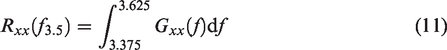
The area from above equation is shown in Figure 8, the root mean square amplitude is square root of the area, they are 22.1, 23.8, and 23.9, respectively, as shown in Figure 7(b).
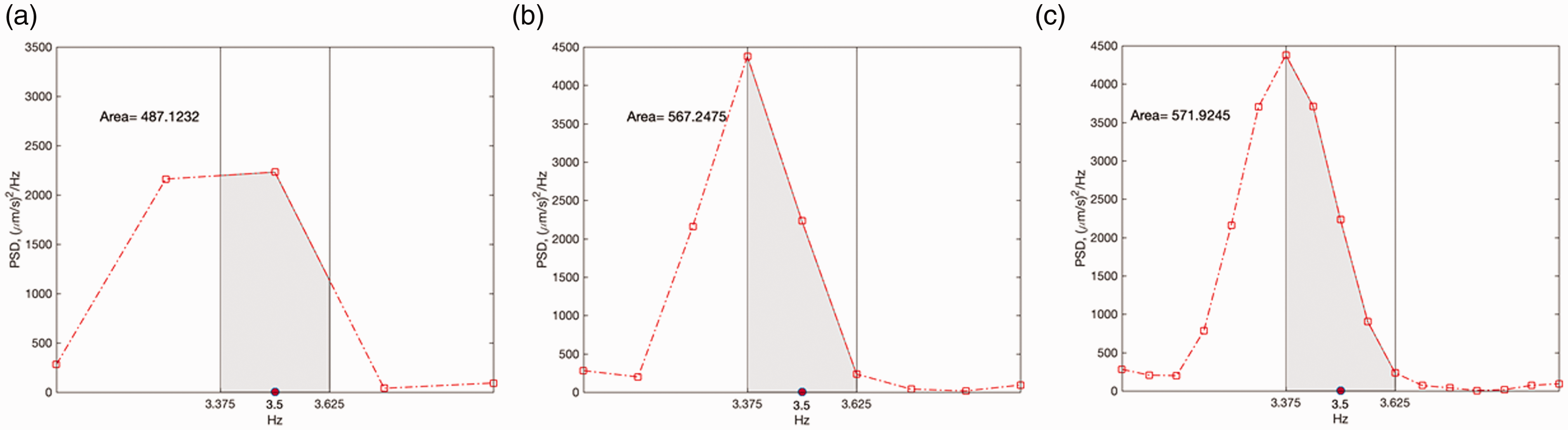
Diagram shows the area from equation (11), (a) 4 s, (b) 4 s + 4 s zeros, and (c) 4 s + 12 s zeros (for case of the center frequency 3.5 Hz as an example).
It is concluded that, for narrowband analysis, a longer duration record (zero-padding) will have high-frequency resolution but may reduce the mean square amplitude which may create a problem for comparison on the result (as shown in Figure 7(a)) unless the result from different frequency resolution can be transformed to the same resolution (as shown in Figure 7(b)). From the result of Figure 7(b) the Cases 2 and 3 can also have the same amplitude as Case 1 which shows that by adding one multiple zero on the original samples length (Case 2) is enough to get good accuracy.
One-third octave band analysis of high-speed train-induced transient vibration of a nearby building
The spectral analysis of structural response induced by high-speed train was studied. Consider a six-story steel structure building located 40 m away from high-speed railway, Figure 9 shows the high-speed train-induced floor response that was measured from the fifth floor of the building and in the direction perpendicular to the high-speed railway.
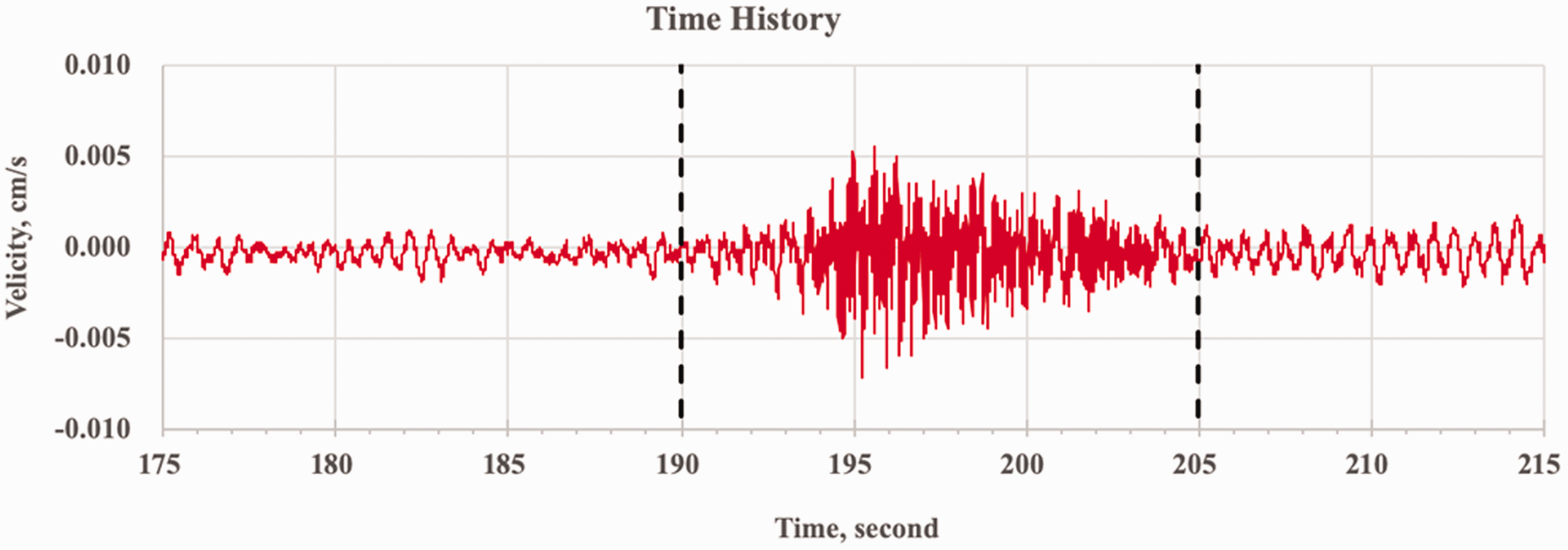
High-speed train induced floor response of nearby building.
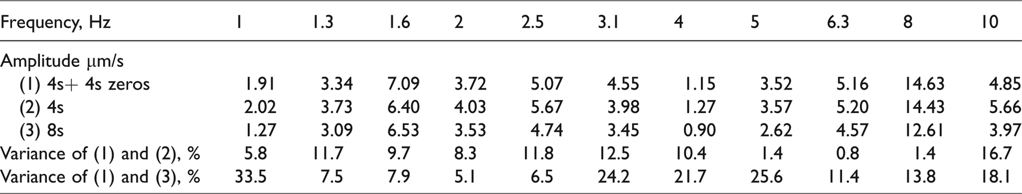
The interval between 190 s and 205 s was selected for analysis by using the procedures of the four cases as described before. Since the duration is 15 s, in contrast to previous analysis, moving window with appending 1 s was used, and peak-hold values of each analysis window were adopted. The one-third octave band amplitude is shown in Figure 10(a), the amplitude ratio of each test case to the Case 2 (4 s + 4 s zeros) is shown in Figure 10(b). One can observe that the longer time period Case 4 (8 s) has the smallest amplitude as compared to other three cases, the amplitude of Case 3 (4 s + 12 s zeros) and Case 2 (4 s + 4s zeros) are almost the same. It implies that by padding one multiple of zeros has good accuracy enough. Table 7 shows the amplitude variance of compared to Case 2 (4 s + 4s zeros).
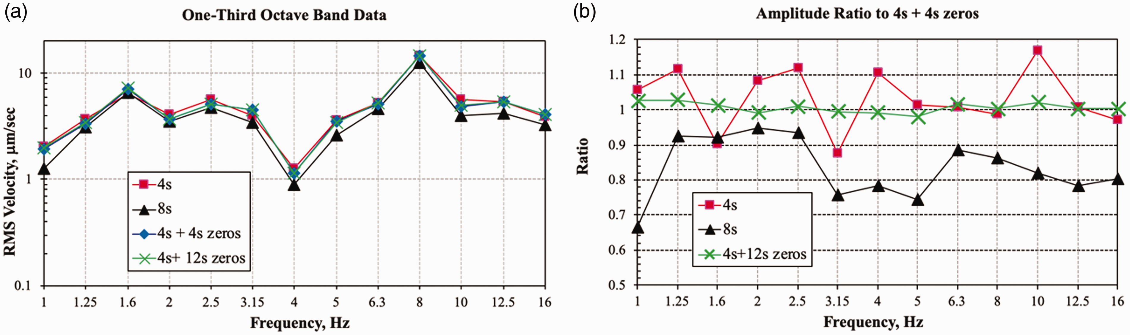
The spectral analysis of high-speed train induced floor response, (a) the one-third band amplitude of four cases and (b) the amplitude ratio to case 4 s + 4 s zeros.
Amplitude variance of three cases of high-speed train induced floor response.
One-third octave band analysis of site ambient vibration
Figure 11(a) is a recorded 64 s ambient vibration data (velocity) of a site. Comparing the one-third octave band of velocity data using three analysis cases, Table 8 shows the parameters of the three cases. From the beginning of the time history, the data of 4 s or 8 s were selected, and then using moving time window by appending 1 s and select another 4 s or 8 s until the last time was shorter than 4 s or 8 s. Thus, the overlap percentage is 75% and 87.5%, respectively. The whole 64 s time history is divided into 64–4 + 1 = 61 and 64–8 + 1 = 57 segments for 4 s and 8 s time intervals, respectively. The result shows the linear average of all segments.
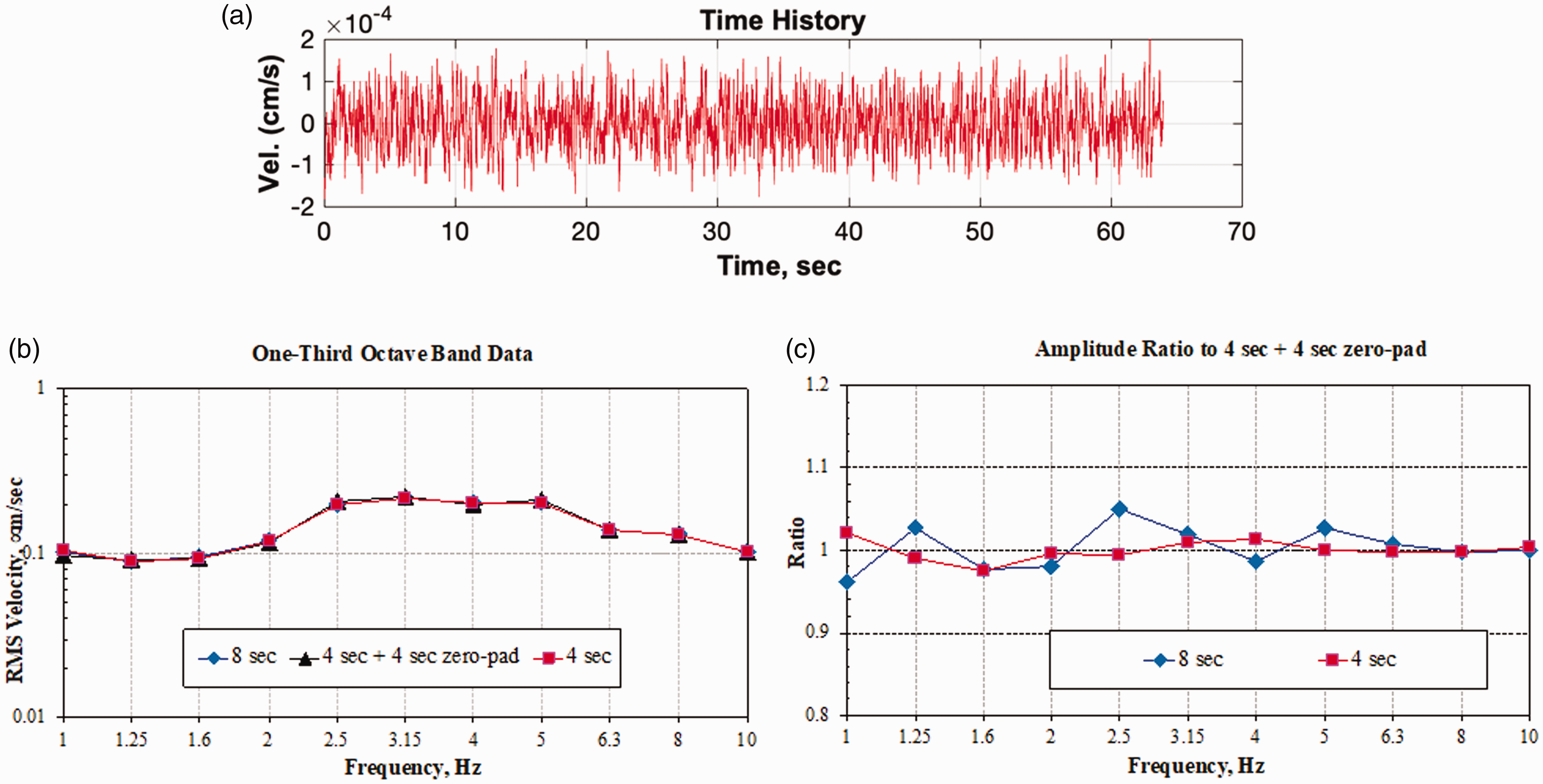
Spectral analysis of site ambient vibration, (a) vibration time history, (b) linear average 1/3 octave band data, and (c) amplitude ratio to “4 s + 4 s zeros.”
Parameters of analysis cases.
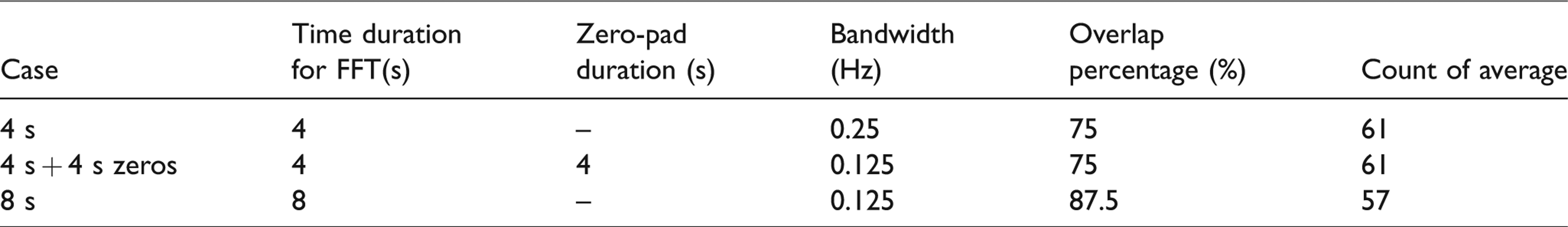
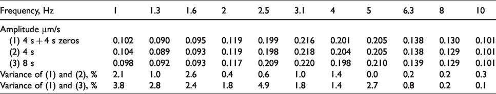
The results of one-third octave band velocity below 10 Hz are shown in Figure 11(b), and the amplitude ratio of case “4 s” and “8 s” to case “4 s + 4 s zeros” is shown as Figure 11(c). Since the ambient vibration can be regarded as stationary vibration signal, we can observe that the three cases have consistent results. The amplitude variance of three cases is within 5% as shown in Table 9. The results demonstrate that for the nearly stationary vibration data, the bandwidth which depends on the time period and zero-padded length is insignificant for spectral analysis.
Amplitude variance of three cases of site ambient vibration.
Conclusions
In this paper, the procedures on the spectral analysis of measured data were discussed by using different time period of zero-paddings at the end of the measured data. Through experimental study on high-speed train induced vibration at free-field, nearby building and ambient vibration were exemplified to demonstrate the procedures of the spectral analysis. Based on the results, some conclusions were drawn and presented as follows: Zero-padding can provide finer bandwidth from shorter time period and get more information/data points of spectrum. From the study, one multiple zero padding of original samples length is demonstrated for getting adequate spectral analysis accuracy. The length of the time period or the bandwidth for spectral analysis of high-speed train induced transient vibration will affect the spectral amplitude. In this study, the amplitude of 4 s time period is 23% higher than 8 s time period from the analysis of free-field data. The amplitude variances further increase at nearby building floor, it results in confusion whether the high-speed train induced vibrations affect the tools installed or not. For a nearly stationary ambient vibration, the length of time period or the bandwidth for spectral analysis is insignificant. The 4 s time period leads to 1/4 = 0.25 Hz bandwidth is too coarse to catch the frequency which peak amplitude happened of a transient signal, the bandwidth 0.125 Hz either by 4 s + 4 s zero or by 8 s time period is more adequate. The selection of bandwidth is crucial for getting comparable amplitude in narrowband analysis. Using different bandwidth may result in extremely opposite amplitudes. For reliable comparison, narrowband spectral analysis had better base on the same bandwidth.
Based on authors’ study, when the sampling rate is 256 Hz, the 4 s samples plus 4 s zeros padded results in 0.125 Hz bandwidth which has better accurate results of spectral analysis either in narrowband or one-third octave band analysis. Therefore, the approach of using a finer bandwidth (0.125 Hz) by adding zeros (4 s zeros) is recommended when one deals with train-induced vibration that spurs up transient amplitudes.
Footnotes
Declaration of conflicting interests
The author(s) declared no potential conflicts of interest with respect to the research, authorship, and/or publication of this article.
Funding
The author(s) received no financial support for the research, authorship, and/or publication of this article.