Modeling of self-excited stress measurement system

Abstract

In the paper two types of numerical models of the self-excited acoustical system are presented. This new type of auto-oscillating system is used for stress change measurement in constructions and rock masses. The essence of the self-excited acoustical system is to use a vibration emitter and vibration receiver placed at a distance, which are coupled with a proper power amplifier, and which are operating in a closed loop with a positive feedback. This causes the excitation of the system. The change of the velocity of wave propagation, which is associated with the change of the resonance frequency in the system is caused by the deformation of the examined material. Stress changes manifest themselves in small but detectable variations of frequency. The first of the presented models was created on the basis of estimating the model parameters by identification of the sensor–conditioner–amplifier–emitter system. The second mathematical model was delivered from the force–charge equation of the piezoelectric transducers: the sensor and the emitter. The model of the loaded beam, which determined the response of any beam point to the force applied to any other beam point is also presented.

Introduction

The speed change of an acoustical wave propagation caused by a stress is tiny. As a result, the need for measuring wave flight (transition) times with a nanosecond accuracy is required. Therefore, the sampling times of GHz range are used in the standard ultrasonic measurement systems. It is possible to work with these values comfortably but only in a laboratory environment: constant temperature, pressure, etc. In practical applications of the ultrasonic strain gauge method, with devices connected to rough and unpolished construction elements in the field conditions, the required measurement accuracy of time of flight is a really demanding task. The same problems may occur in other ultrasonic diagnostic systems where the propagation time is a mean of materials state assessment. ¹

Currently there are several interesting researches in the field of system stress change measurement and in structural health measurement. The application of carbon nanotubes (CNTs) can be distinguished in nanoscale stress measurement. A study on the deformation and electrical effects of a CNT–epoxy resin composite is presented in Paćko et al. ² The principle of operation of this method is that with the deformation of the composite the CNT alignment in the matrix is changing. It influences on the electrical properties of the nanotube. The method is still under research because of the presence of various effects, which may cause some undesired measurement results.

There is also application of optic fiber for stress change measurement. ³ In the method two light beams with different frequencies transferred antiparallel to a fiber are used. The acoustic waves moving in the optical fiber core are excited as a result of interaction between them. According to the Doppler’s effect, change of stress causes change of frequency. Unfortunately, this method requires very wide range of frequency to operate properly.

Another method uses RFID sensing technology in structural health monitoring. ⁴ The sensors work in wireless technology with possibility of interrogation from distance with the antenna applied additionally for energy harvesting.

In this paper a self-excited acoustical system (SAS) was developed. The essence of the SAS system is to use a vibration emitter and a vibration receiver placed at a distance, which are coupled with a proper power amplifier and are operating in a closed loop with a positive feedback. This causes the excitation of the system. The change of the velocity of wave propagation, which is associated with the change of the resonance frequency in the system is caused by the deformation of the examined material. Stress changes manifest themselves in small but detectable variations of frequency. The SAS system allows to operate in the range of a dozen or so kHz which is easily reached in practical applications. It is attainable by using the self-excitation phenomena.

The self-excited systems are widely known in technics ³ and in energy-harvesting devices.^5–7 The self-excitation is used also in devices called auto-oscillators.

SAS system as every auto-oscillator consists of three main parts: energy source, oscillating system, and control valve of energy supply.^8,9 The scheme is presented in Figure 1. The system can be divided essentially into two parts: the first one is a sample under examination (mechanical system part) and the second one is equipment (executive system part). The latter consist of measurement and vibration transducers as well as a control part. The emitter (E) is a piezoelectric shaker while receiver (R) is a piezoelectric accelerometer. A conditioner and an amplifier are used adequately to condition and amplify the signal obtained from the receiver. The emitter, the conditioner, and the amplifier with the shaker at the end create a positive feedback loop. Additionally, the data acquisition card and FPGA unit are placed in the loop. Their task is to gather the data and control the system by controlling the delay time of the loop. The parameters of the shaker and the receiver are presented in Table 1.

Figure 1.

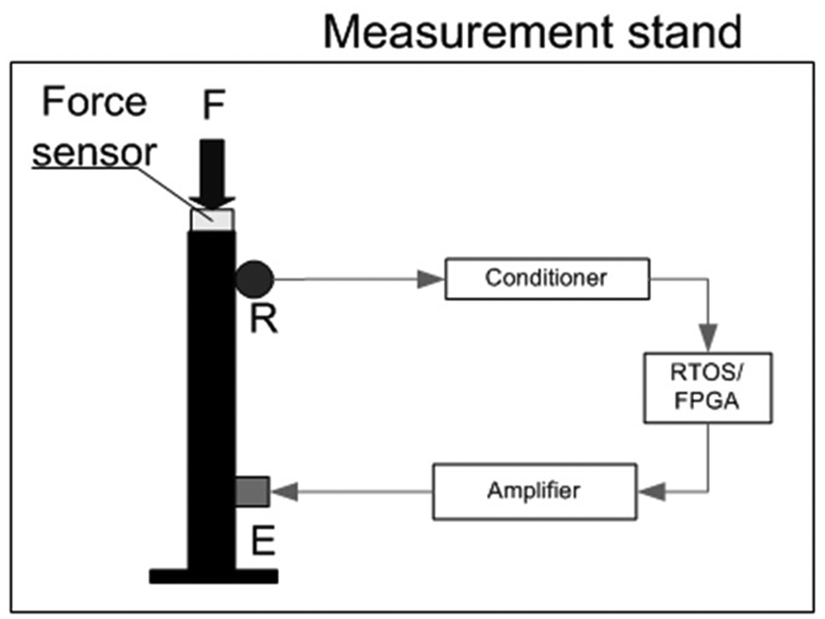
The scheme of the SAS: E: emitter; FPGA: Field programmable gate arrays; R: receiver; RTOS: Real-time operating system.

Table 1.

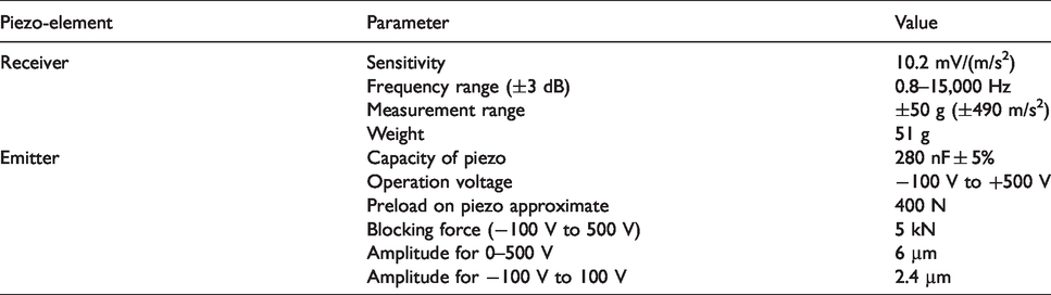
Parameters of the piezo-elements.

Piezo-element	Parameter	Value
Receiver	Sensitivity	10.2 mV/(m/s²)
	Frequency range (±3 dB)	0.8–15,000 Hz
	Measurement range	±50 g (±490 m/s²)
	Weight	51 g
Emitter	Capacity of piezo	280 nF ± 5%
	Operation voltage	−100 V to +500 V
	Preload on piezo approximate	400 N
	Blocking force (−100 V to 500 V)	5 kN
	Amplitude for 0–500 V	6 µm
	Amplitude for −100 V to 100 V	2.4 µm

Every part of the loop is characterized by some delay time which is out of control. However, adding some additional delay time enables to control the self-excited frequency range. The whole control system was programmed in the LabVIEW software.

The physical laws of the self-excited systems allow to conclude that the longer flight time through the tested subject is the lower frequency at which excitation occurs. ¹⁰ More details regarding the self-excited systems have been presented by Astashev and Babitsky. ¹¹

The ideas described in Skrzypkowski et al. ⁹ and Lalik et al. ¹² allowed the authors to analyze the influence of construction effort on the delay time in the mechanical part of the system. Therefore, the influence of a stress in the sample on the system resonance frequency is also known.

Self-excited acoustical system (SAS) for monitoring the change of the stress at the tested construction uses the acoustoelastic phenomena. The essence of the SAS system is to use a vibration exciter and vibration receiver placed at a distance, which are coupled with a proper power amplifier, and which are operating in a closed loop with a positive feedback. This causes the excitation of the system. The change of the speed of wave propagation, which is associated with the change of the resonance frequency in the system, is caused by the deformation of the examined material. The real test stand of the SAS system is presented in Figure 2.

Figure 2.

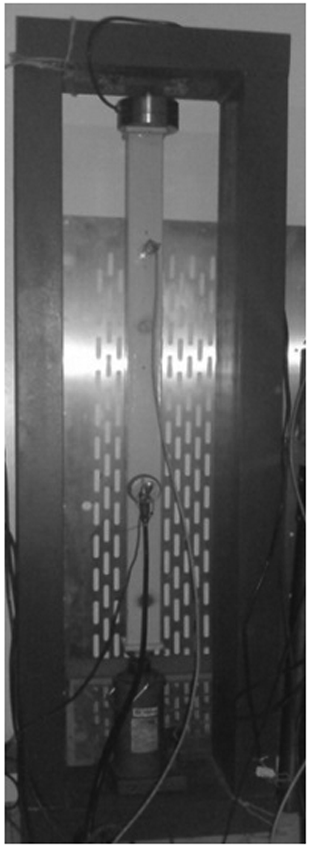
The real test stand.

Mechanical vibrations were introduced to the tested beam by the piezoelectrical exciter and then received by the accelerometer. The signal was then conditioned, amplified, and then transmitted back to the exciter. The configuration led to formation of self-excited vibrations of a specific frequency (its limit cycle). The frequency varied with a change of the degree of stress–strain state in accordance with the acoustoelastic effect. ¹³ Measurement of self-excitation frequency made it possible to give an indirect assessment of the stress–strain state degree of the tested structure.

The main purpose of the presented study was to find a relationship that would allow correlating the frequency of the SAS system with the load on the beam under examination. For this purpose, two models of the entire test stand were built. The reverse model consisted of conducting an identification experiment in an open loop system. By using parametric models, the identification of the transmittance parameters of individual elements of the measuring system and the tested beam was possible. A mathematical reference model was also created. It was created by joining mathematical models of individual components of the test stand. The beam model was based on dispersion equations. The piezo-element models were created based on the electronic equivalent of an ultrasonic transducer with negistor shown in Figure 3.

Figure 3.

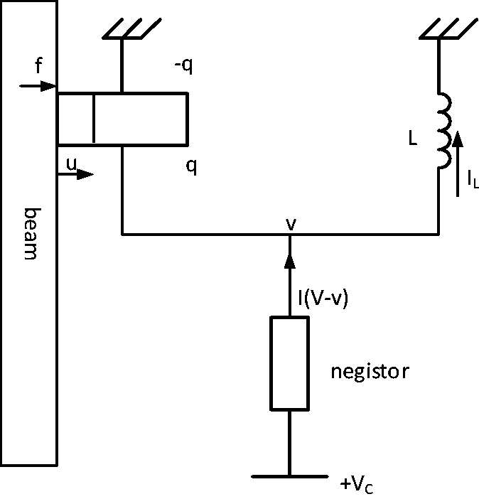
Scheme of the electrical equivalent of the self-excited system, where V_C is the static supply voltage, I is the current, q is the charge, f is the mechanical force, v is the potential drop, u is the displacement, L is the inductance, and I_L is the current in the inductor.

The aim of the study was to compare the results recorded by two different measuring systems (via traditional strain gauge system and innovative SAS system) to assess the strain of the construction by using a non-destructive method with two proposed models.

Laboratory test results

If the feedback loop works with a well-matched gain factor, the sample under examination is in the resonance state. After initial excitation of the sample the tensile force in the sample is changed by a hydraulic jack (Figure 2). The jack acts on the basis of the frame with an additional massive stone extension. It causes variable tensing on the sample. The load is measured by the strain gauge sensor. Both the emitter and the receiver can be fixed to different places of the sample.

The entire system can be easily explained by the phenomenon of resonance. In the positive feedback loop the instability will always occur. ¹⁴ The system, in which no restrictions occur in elements of the loop (e.g. saturation of electronic components) and the beam dissipates the mechanical energy in a linear manner, always increases the amplitude of its oscillation. ¹⁵

However, if one of these conditions is not fulfilled, it results in limitations of the signal, or in other words, in reaching a stable limit cycle. Then the system operates in its border cycle and a stable oscillation is achieved. These oscillations have constant amplitude and the frequency is strictly connected with the change of time of flight delay (TOFD). TOFD is also related to the change of velocity of acoustic wave in the studied material. This change, in turn, is strongly determined by elasto-acoustic coefficient, which changes with the stress. The Fourier transform detects the change of this frequency. The change of the frequency from about 7900 to 8300 Hz corresponding to the change of the load from 0 N to 50 kN of the beam under examination in the real test stand (Figure 2) is presented in Figure 4.

Figure 4.

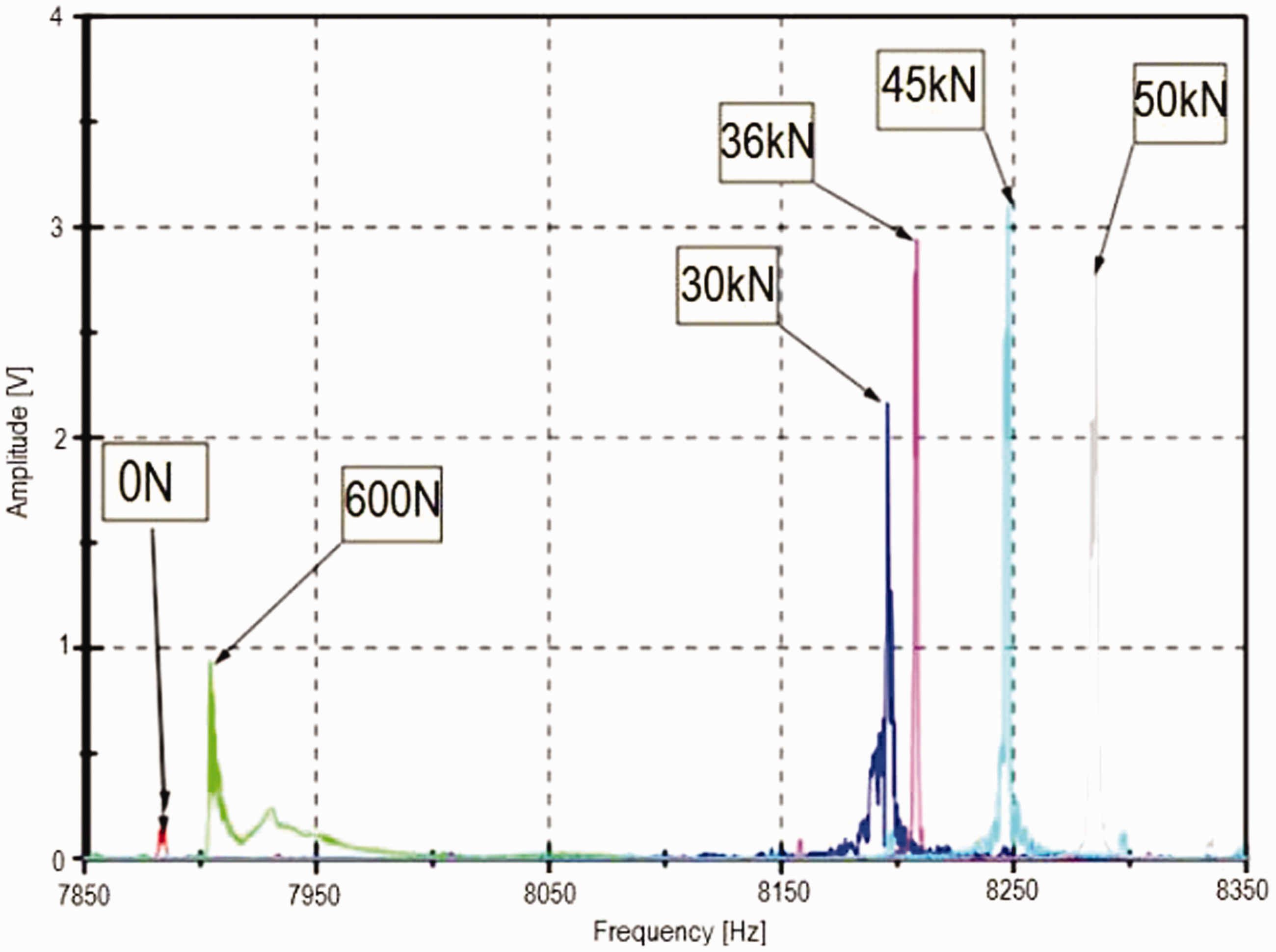
Change of the frequency corresponding to the change of the load of the beam under examination.

The main idea behind operating the SAS system is the frequency measurement of the execution system which depends on the delay in the sample. The material effort of the sample influences the flight time (delay time) and consequently the system resonance frequency.

The simple equation proposed in equation (1) describes the relation between the velocity of wave propagation and a stress change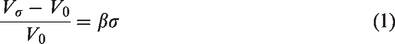

$$\frac{V_{\sigma }-V_0}{V_0}=\beta \sigma$$

(1)

where $V_0$ is the velocity of wave propagation in the measurement area without stress, $V_{\sigma }$ is the velocity of wave propagation in the measurement area with stress σ, and β is the value of elasto-acoustic coefficient. It depends mainly on a chemical composition of material and a material heat treatment as well as on a direction of wave propagation and a direction of molecules vibration in relation to a stress direction.^16,17

On the other hand, the delay time is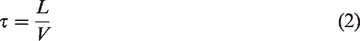

$$\tau =\frac{L}{V}$$

(2)

where L is the distance between an emitter and a receiver, τ is the delay time of a wave flight, and V is the velocity of wave propagation.

After substituting equation (1) into equation (2), equation (3) was delivered. It describes the relation between the change of the flight time and the change of stress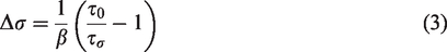

$$\mathrm{\Delta }\sigma =\frac{1}{\beta }\left(\frac{{\tau }_0}{{\tau }_{\sigma }}-1\right)$$

(3)

where $\mathrm{ }\mathrm{\Delta }\sigma$ is the change of the stress in beam under examination $,\mathrm{ }{\tau }_0$ is the TOFD for sample with no compression or with preliminary load, and $\mathrm{ }{\tau }_{\sigma }$ is the time of acoustic wave flight for the compressed beam.

The derived equation (3) shows that the distance between the exciter and emitter is irrelevant in stress change measurement.

To sum up, after closing the positive feedback loop, the SAS system will achieve vibrations of its limit cycle at a certain frequency. This frequency depends only on the time of flight of the wave, that is the delay in which wave passes between the emitter and the receiver. This delay, in turn, depends on the relative elongation and elasto-acoustic coefficient β (equation (3)), as well as the oscillation form of the beam under examination. The first two parameters depend directly on the force loading the beam and are continuous in the elasticity range of the tested material. Hence, it can be concluded that by reading the frequency of the SAS system it is possible to determine the load of the tested material.

However, the third parameter, which is a form of vibration of the beam, should be investigated. It causes discontinuous, abrupt changes in the time of flight of the wave, which results in abrupt changes in the frequency of the SAS system. The system without additional circuits (e.g. phase tracking, filters) decides by itself on the choice of a specific type of transmission wave among these which have been introduced into the tested material by the emitter. Commonly, these are the waves which have the highest amplitude. Unfortunately, along with the change in the load of the tested material, the amplitudes of these waves also change. It can result in a sudden change of the SAS system frequency due to use of another form of beam oscillations (Figure 5). The presented behavior of the system is certainly undesirable. Together with visible “frequency shifts” and thus the oscillation form changes, it is impossible to determine exactly the stress in the sample. The additional digital filters based on FPGA technology are under construction to eliminate the effect.

Figure 5.

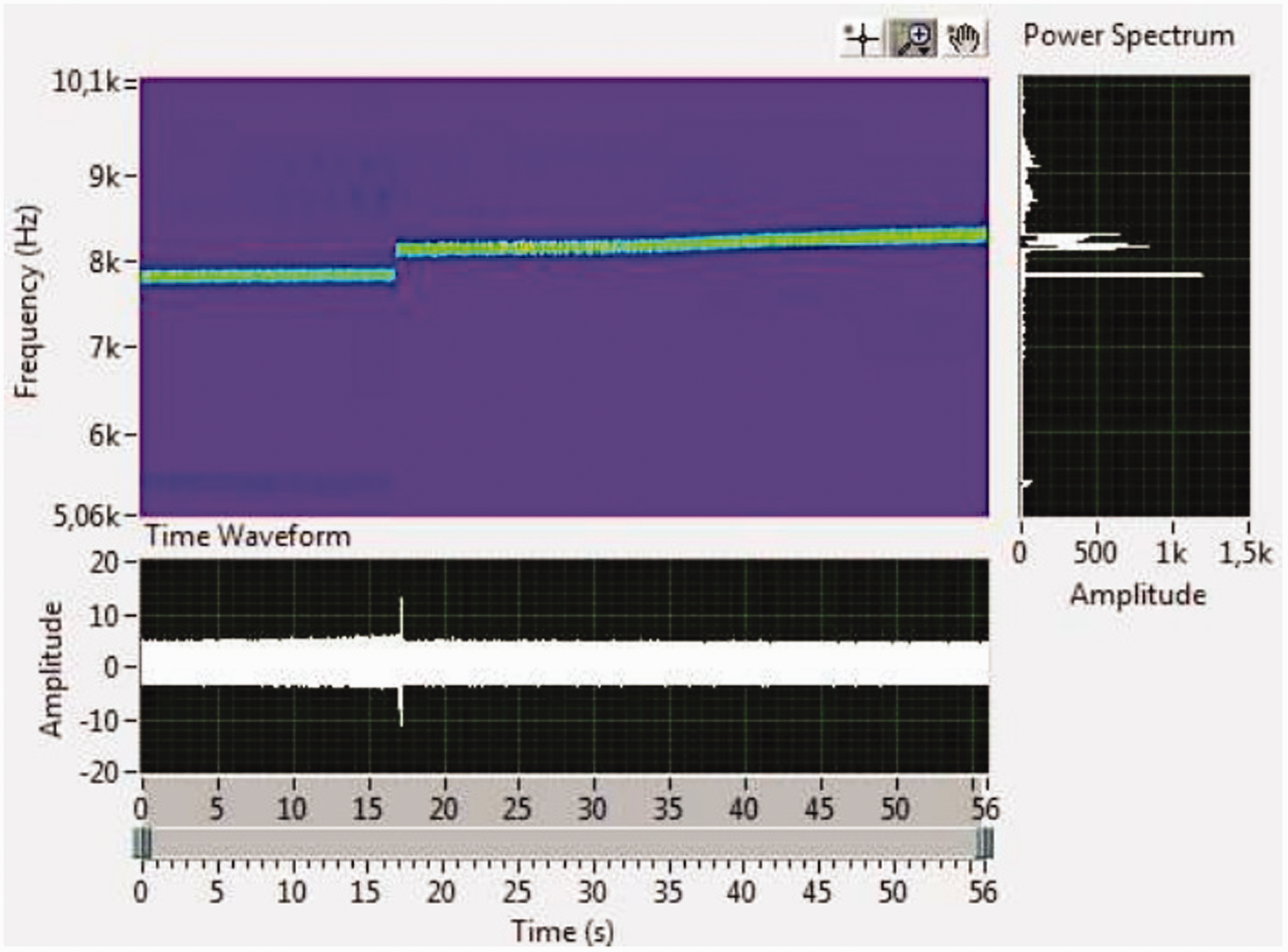
Short time-frequency Fourier transform for the SAS signal from the tested beam.

The sample under examination was a metal beam compressed axially by the force in the range of 5–50 kN. The maximum vibration amplitude was 5 µm. During laboratory tests the SAS signal sometimes changed its value randomly. It occurs in the spectrogram (Figure 6) as a “shift” from one resonance frequency to the other. The figure shows the frequency change of the auto-oscillator system made by the stress change in the sample. Along with the time (visible on the axis of abscissa) the stress increased steadily. At the beginning for a minimum load of 5 kN applied to the sample, the resonance frequency was 7891 Hz. In 17 s with 10 kN load a clear shift was visible, due to the oscillation form change. The frequency changed to 8101 Hz. Further load increase to 50 kN resulted in a steady increase of the resonance frequency to 8273 Hz. The whole increase of the resonance frequency was 172 Hz for the range of 10–50 kN load.

Figure 6.

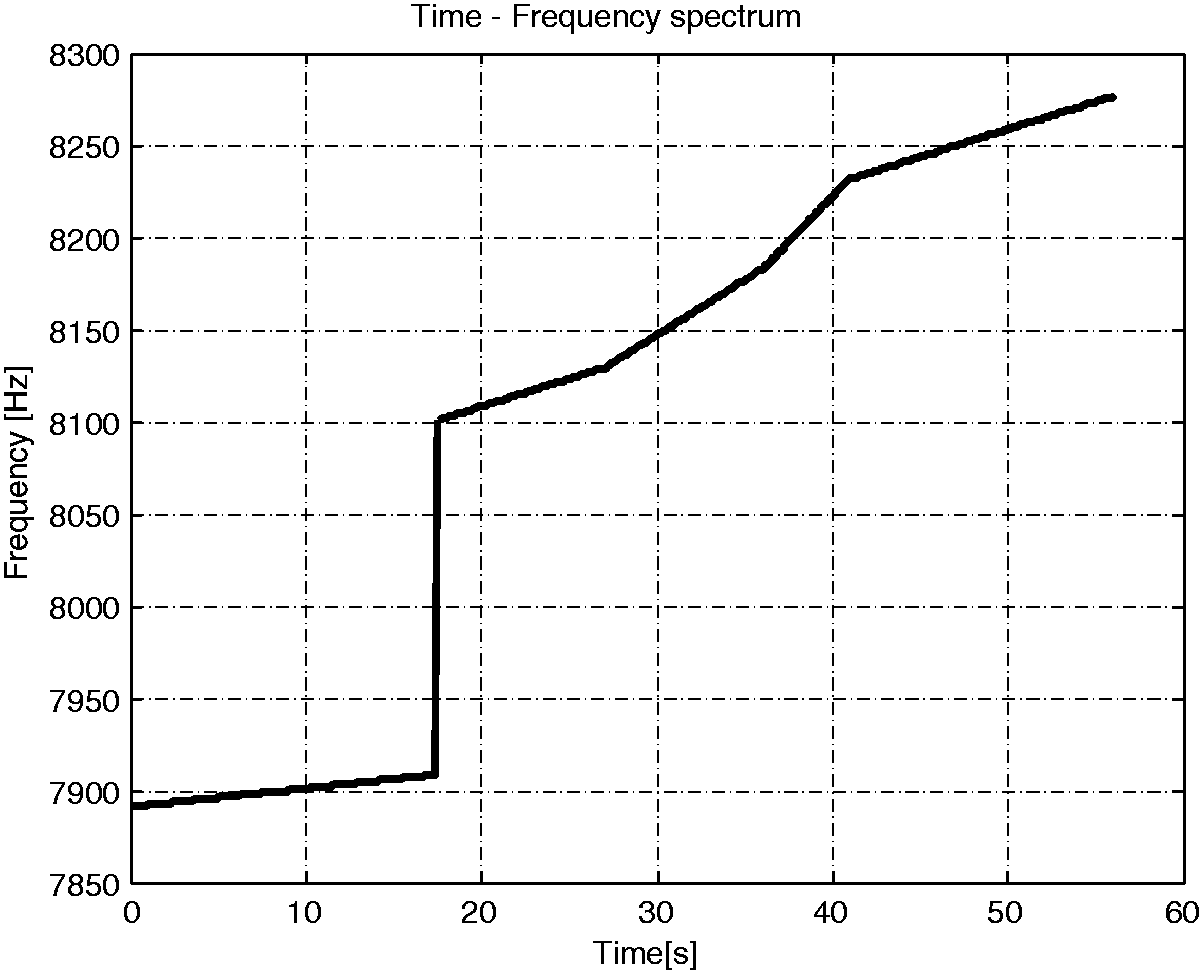
Time-frequency spectrum for the laboratory test.

Reverse model of the SAS system

Figure 7 presents the structure of the numerical model of the SAS system. The main point of the research was to find the parameters of transmittance for each element shown in the model. The autoregressive with exogenous input (ARX) model was used to create the reverse model of the SAS system to reach this goal. The ARMAX and Box–Jenkins parametrical model were also tested, but their fit was insufficient. ¹⁸

Figure 7.

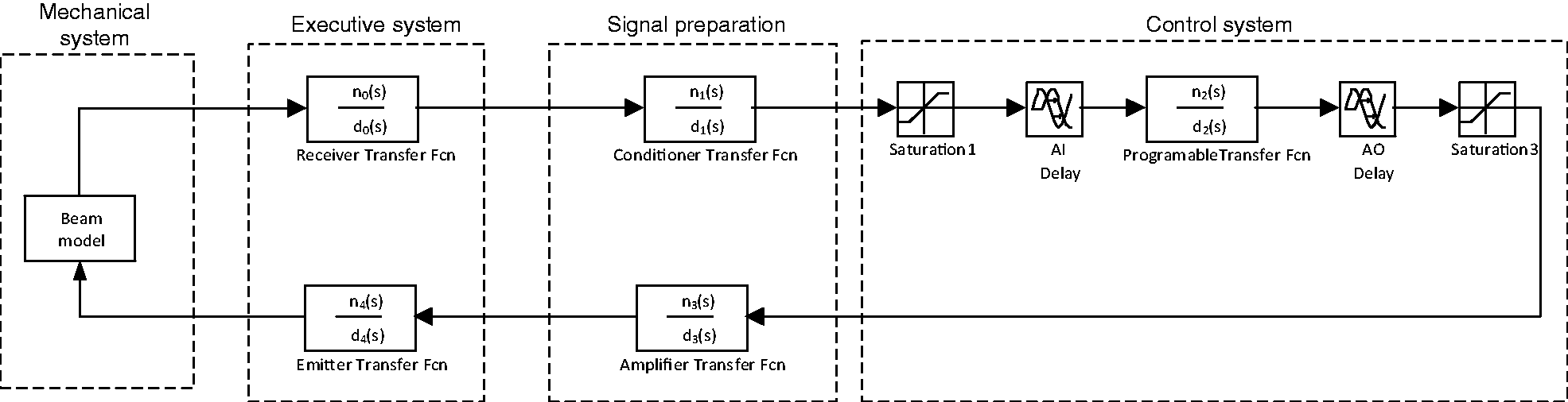
Numerical model of the SAS, where n_i and d_i are corresponding to numerator and denominator of appropriate element of transfer function. AI: ▪; AO: ▪.

Figure 8 presents the structures of parametrical models used in the identification process.

Figure 8.

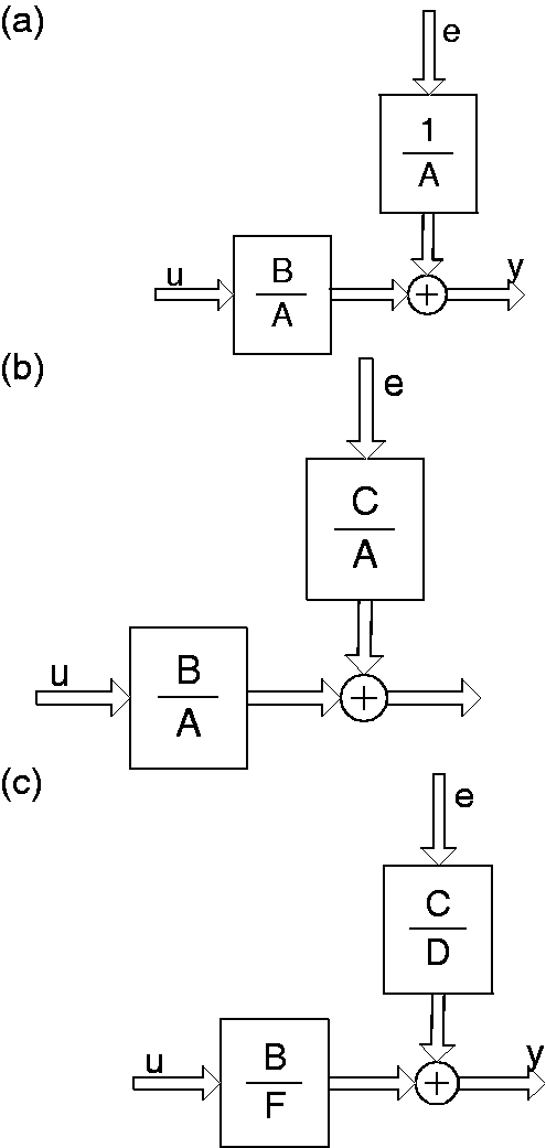
The structure of the parametrical models: (a) ARX, (b) ARMAX, and (c) Box–Jenkins.

The first step in identification is always an experiment with open loop system and recording of excitation signal and system response. The structure of the open loop system used for the identification of parameters is presented in Figure 9. The accelerometer signal was chosen as the input signal of the structure. The outputs were the vibrations created by the shaker. Both signals with sampling of 100 kHz were measured and analyzed, which is presented in Figure 10. By using the parametrical model identification, the unanimity of 99% was reached. In the next step, the found transmittance was used to create the model of the feedback system.

Figure 9.

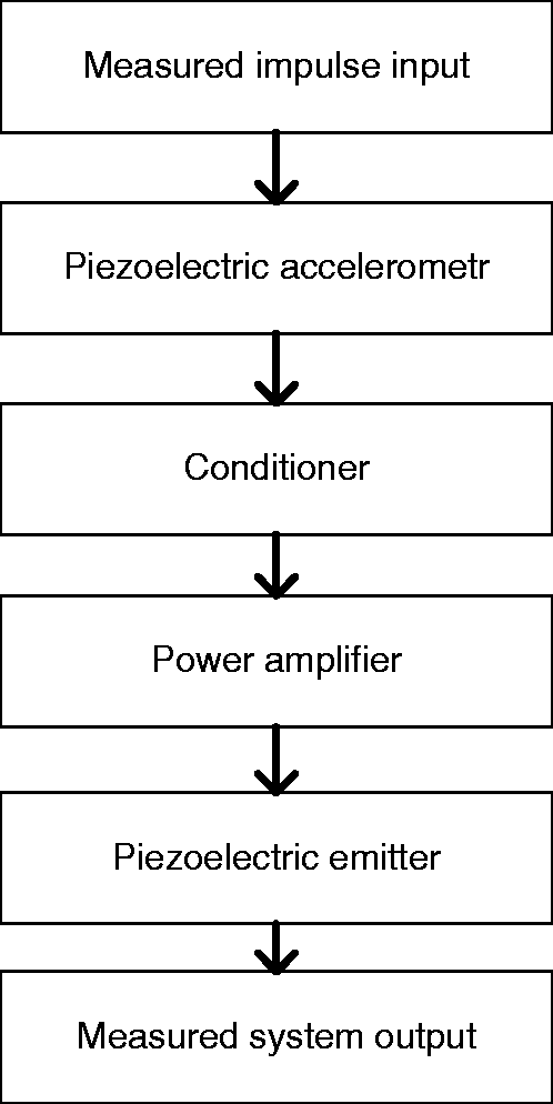
The structure of the open loop system used for the identification of parameters.

Figure 10.

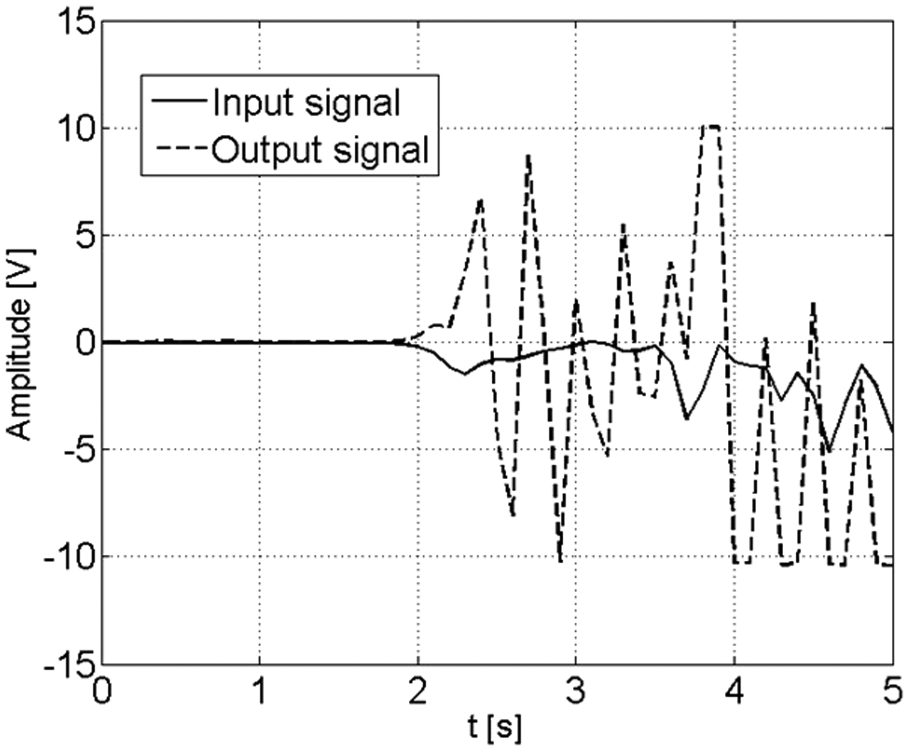
The open loop system impulse response.

The sample was modeled as a beam which dissipates the vibration energy supplied to it and also is seen as the delay in the feedback. The whole executive system (the SAS equipment) was implemented as the reverse model based on the presented parametrical identification. Additionally, the saturation block was used to limit the range of the system signal.

In Table 2 the unanimity between the parametrical models and the real system is shown. The parameters such as n_a, n_b, n_c, n_d, and n_f are the orders of the particular polynomials presented in Figure 8. The parameter n_k is a number of input samples that occur before the input affects the output—known also as the dead time of the system. Ultimately, the ARX model with the polynomial A of degree 15 and the polynomial B of degree 12 was chosen, as the most fitting and relatively simple.

Table 2.

The comparison between the parametrical models.

Parametrical model	Structure	na	nb	nk	nc	nd	nf	Fit (%)
ARX	Ay=Bu+e	4	4	1				27.86
		8	6	1				36.66
		10	8	1				39.81
		12	10	1				60.79
		12	8	1				63.89
		15	10	1				81.14
		15	11	1				98.25
		15	12	1				99.54
ARMAX	Ay=Bu+Ce	2	2	1	2			3.43
		4	2	1	2			14.01
		4	4	1	2			30.97
		8	4	1	4			29.61
		12	10	1	4			48.26
		15	10	1	4			96.75
		15	12	1	4			99.33
		15	12	1	8			99.35
Box–Jenkins	Ay=[B/F]u+[C/D]e		8	1	4	2	2	2.46
			10	1	10	5	5	6.23
			8	1	8	2	2	13.01
			8	1	8	8	8	16.66
			2	1	2	2	2	21.10
			4	1	4	2	2	24.56
			8	1	8	4	4	25.45
			10	1	10	8	8	25.61

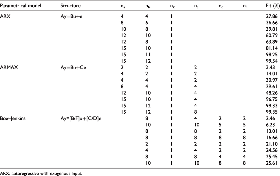
ARX: autoregressive with exogenous input.

The unit circle shown in Figure 11 presents the zeros and poles for the model transfer function. Both of them may be outside the unit circle. This state indicates the system instability, which is consistent with the time-domain characteristic shown in Figure 12. An energy dissipation element responsible for the stability of the system is a beam under the load. ¹⁹ The conversion between an electrical and mechanical energy takes place in piezo-elements of the system and this energy is later dissipated as heat and sound. This mechanism occurs in a beam. This way the SAS system can reach a stable limit cycle, where the instability of the open loop reverse model is eligible.

Figure 11.

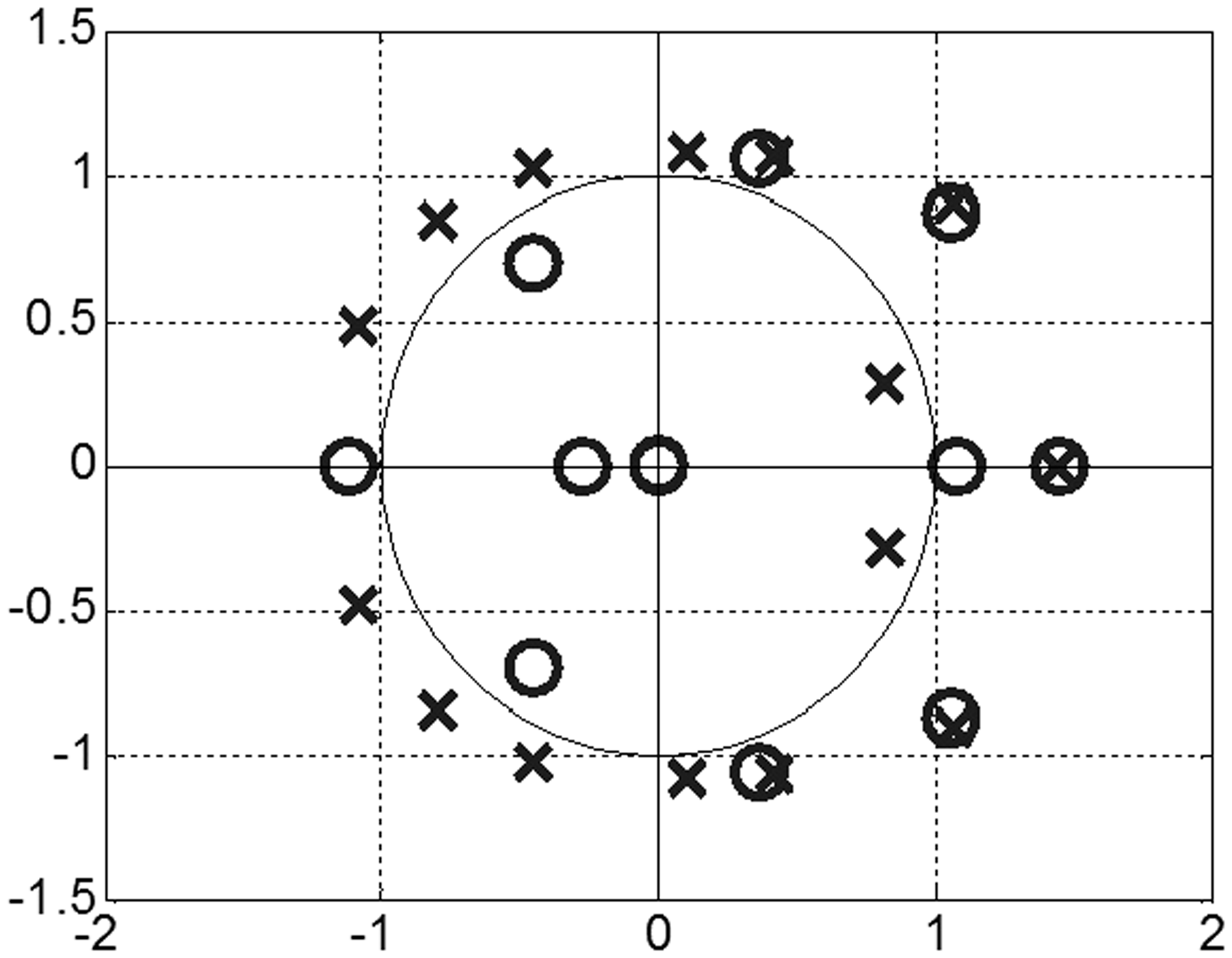
Unit circle for discrete object transmittance. Poles (x) and zeros (o).

Figure 12.

Unstable model operation for the linear beam and execution system.

One of the major features of self-excited systems is their nonlinearity. An auto-oscillator is a nonlinear dynamic system, in which both the amplitude and frequency of oscillations may remain constant over a long time. The parameters of the system are determined by the system itself and are characterized by a high autonomy, even despite initial conditions. ²⁰

In the self-excited systems operating under the influence of the external harmonic force, the quasi-periodic state is reached due the extortion presence. The extortion frequency is close to the frequency of the auto-oscillator. Figure 12 shows the operation of the unstable model for the linear beam and the execution system. The auto-oscillator nonlinearity is the essential parameter, which during the excitation causes the growth of the oscillation amplitude, while the system operates at its stable limit cycle after stopping the excitation. The easiest way to model the nonlinearity is to use the saturation of the electrical signal. The chart showing the vibration (including the saturation) is presented in Figure 13.

Figure 13.

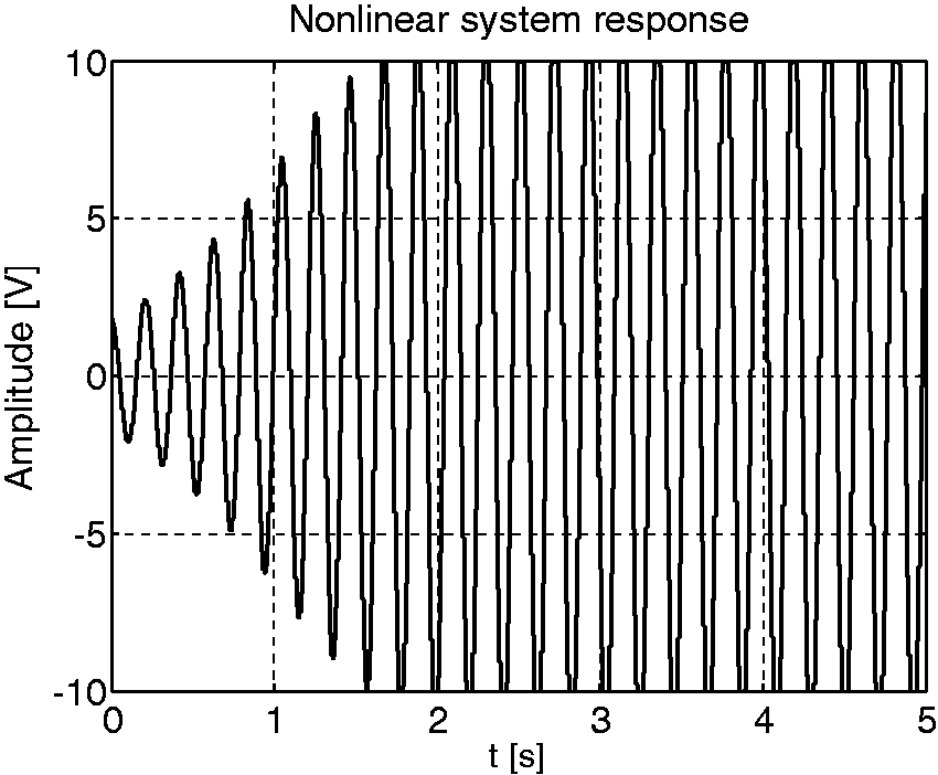
The stable model operations for nonlinear beam and the executive system with saturation.

An additional nonlinearity can be entered to the system by using the model of the beam under load. It has a different gain factor of an input vibration amplitude which depends on the amplitude of these vibrations itself. As a result, the system is attracted to certain state and then remains in the stable limit cycle. The phase diagram for the SAS system is shown in Figure 14.

Figure 14.

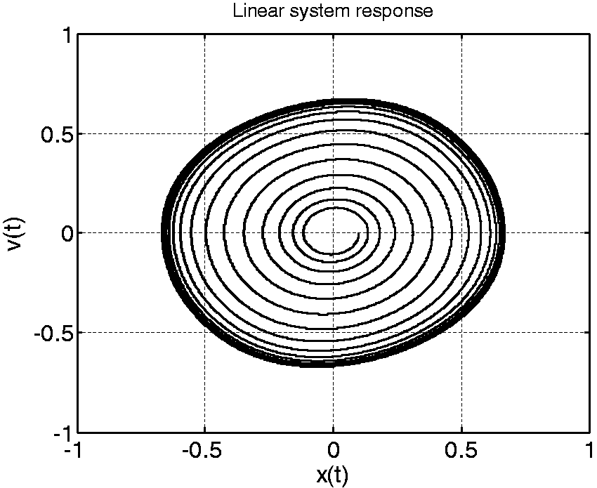
The stable limit cycle for the SAS model.

Model of execution system

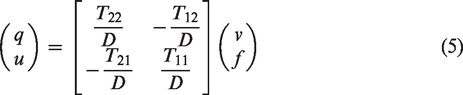
A passive piezoelectric stack may be represented in an acoustical system as a MIMO system with two inputs and two outputs (4). A drop of potential v and a piezoelectric charge q are the inputs of the system. A mechanical displacement u and mechanical force f are the system outputs. Obviously, for the sensorial operation of the piezoelectric element, the inputs and outputs would be swapped. According to the theory presented in equation (16), the relationship between inputs and outputs may be represented by equation (4) for the sensorial operation and equation (5) for the actuating operation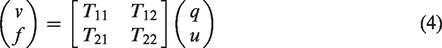

$$\left(\begin{array}{c}v\\ f\end{array}\right)=\left[\begin{array}{cc}{T}_{11}& T_{12}\\ T_{21}& T_{22}\end{array}\right]\left(\begin{array}{c}q\\ u\end{array}\right)$$

(4)

$$\left(\begin{array}{c}q\\ u\end{array}\right)=\left[\begin{array}{cc}\frac{T_{22}}{D}& -\frac{T_{12}}{D}\\ -\frac{T_{21}}{D}& \frac{T_{11}}{D}\end{array}\right]\left(\begin{array}{c}v\\ f\end{array}\right)$$

(5)

where D = T₁₁T₂₂−T₁₂T₂₁ is the determinant of the matrix T. T₁₁ can be interpreted as the inverse piezoelectric capacity, when the piezo-element is not deformed. T₂₂/D can be interpreted as the capacity of the piezo-stack, when there is no compressing force on it. T₁₂ is the mechanical stiffness of the stack. It is required that T₁₂ = T₂₁.

In order to create a physical model of the piezo-stack transducer, the condition to maintain the current should be met (equation (6)), where q is the charge, v is the drop of potential, I_L is the piezo-stack coil current, V_C is its polarity static voltage, and I is the current through the negistor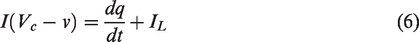

$$I\left(V_c-v\right)=\frac{dq}{dt}+I_L$$

(6)

The authors in Liehr et al. ³ postulated that equation (6) has a stable solution for v = q = 0 and I_L=I(V_C), hence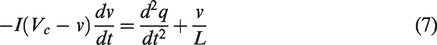

$$-I\left(V_c-v\right)\frac{dv}{dt}=\frac{d^{2}q}{d{t}^2}+\frac{v}{L}$$

(7)

where L is the inductance of the stack.

Substitution of equation (7) into equation (5) gives a dependence between the mechanical input force f and the voltage change for the output v in the sensorial operation of the piezo-stack

$$\frac{d^{2}v}{d{t}^2}-\epsilon (1-3\beta v^2)\frac{dv}{dt}+\frac{1}{LC}v=\frac{T_{12}}{T_{22}}\frac{d^{2}f}{d{t}^2}$$

(8)

where parameter ε describes the strength of the negative resistance of the lambda diode used in electrical equivalent model of the auto-oscillating system, $\mathrm{ }\beta$ describes curvature at the inflection point, and C is the capacitance provided by the piezoelectric transducer and its cables.

The dependence for the actuating mode can be derived in analogy to equation (8). Both types of activities have been included in development of a model of the SAS system. The simulation results are presented in the “Verification of simulation results” section.

Beam model

The SAS system model can be completed only after considering the mechanical part of the measurement system. A beam model used to determine the acoustical wave transfer function is shown in Figure 15. According to the theory presented in equation (9), based on dispersive equations—in this case, considering only transverse wave, the response of any point of the beam in function of the force applied to certain other point of the beam can be modeled. The dispersion equation, which describes the properties of transverse waves, can be determined by using the relation

$$\mu \frac{{\partial }^{2}w(x,t)}{\partial t^2}+P_0\frac{{\partial }^{2}w(x,t)}{\partial x^2}+EJ\frac{{\partial }^{4}w(x,t)}{\partial x^4}=f(x,t)$$

(9)

where μ is the linear density of the beam, Ε is the Young’s modulus, J is a cross-sectional moment of the inertia, and P₀ is the force causing initial stress in the beam. Function w(x,t) describes a transverse wave and f(x,t) is an external force applied to the beam.

Figure 15.

The measurement stand beam configuration.

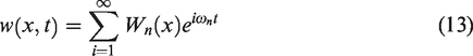
The monochromatic wave was taken under consideration in order to determine the dispersion equation. It can be described by the following equation

$$w\left(x,t\right)=W_0\mathrm{s}\mathrm{in}(\omega t-kx)$$

(10)

where ω is the wave angular frequency and k is a wavenumber. Symbol W₀ represents the magnitude of the transverse wave.

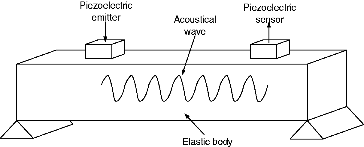
Assuming that in the beam length l occurs n waves, then the wave number can be derived from relation

$$k=\frac{2\pi n}{l}$$

(11)

The natural frequency of the beam 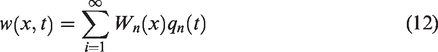${\omega }_n$ under the transverse vibration can be described as

$$w\left(x,t\right)=\sum _{i=1}^{\mathrm{\infty }}{W}_n\left(x\right)q_n\left(t\right)$$

(12)

where $\mathrm{ }{q}_n\left(t\right)\mathrm{ }$ is a time-dependent generalized variable and $W_n\left(x\right)$ is the transverse mode shape corresponding to each natural frequency. Equation (12) can be also represented in a complex form

$$w\left(x,t\right)=\sum _{i=1}^{\mathrm{\infty }}{W}_n\left(x\right)e^{i{\omega }_{n}t}$$

(13)

The differential equation for the modal coordinate q₁ of the bar can be obtained using Lagrange’s equations. ²¹ Therefore, one degree of freedom beam model can be approximated by equation (14)

$${\ddot{q}}_1\left(t\right)+2\zeta {\omega }_n{{\dot{q}}_1+\omega }_n^2{q}_1\left(t\right)=f\left(t\right)\kappa$$

(14)

where ζ is the dimensionless damping factor, ω_n is the damped natural frequency of the beam, f(t) is the mechanical force produced by the piezo-actuator, and κ is the normalized mode shape amplitude.

The beam model described in equation (14) does not determine the influence of the compressive force P₀ in a complex SAS system model. The relation in equation (13) can be substituted into equation (9), where in a case of free vibrations of the beam without actuator: f(x,t) = 0, the equation describing the dispersion properties of transverse waves can be obtained.

Equation (15) determines the relationship between a damped natural frequency of the beam ω_n and the compressive force P₀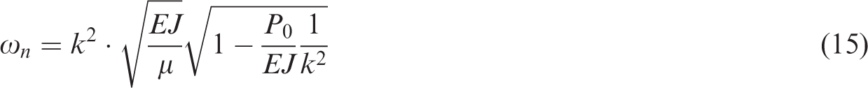

$${\omega }_n=k^2·\sqrt{\frac{EJ}{\mu }}\sqrt{1-\frac{P_0}{EJ}\frac{1}{k^2}}$$

(15)

When substituting the dependence (11) into equation (15), the relationship (16) is obtained. It presents the dependence between natural frequency of the beam and the compressive force for nth mode shape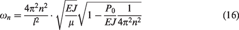

$${\omega }_n=\frac{4{\pi }^2{n}^2}{l^2}·\sqrt{\frac{EJ}{\mu }}\sqrt{1-\frac{P_0}{EJ}\frac{1}{4{\pi }^2{n}^2}}$$

(16)

Equation (14) describes the mechanical part model of the measurement stand. The combination of the mechanical part model and the executive system models (invert and simple) together with the control system allowed to simulate the whole SAS system behavior. Equation (16) can be used to determine the relationship between the beam compressive force and the frequency of the SAS system itself. The results of the simulations are gathered in Table 3 and are presented in Figure 16.

Table 3.

The comparison between measurement results and the model simulation.

Compressive force (kN)	Measurements (Hz)	Inverse model (Hz)	Mathematical model (Hz)
5	7891	8050	8042
10	8101	8105	8093
20	8142	8145	8135
30	8201	8199	8191
40	8241	8240	8235
50	8273	8280	8265

Figure 16.

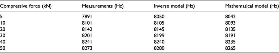
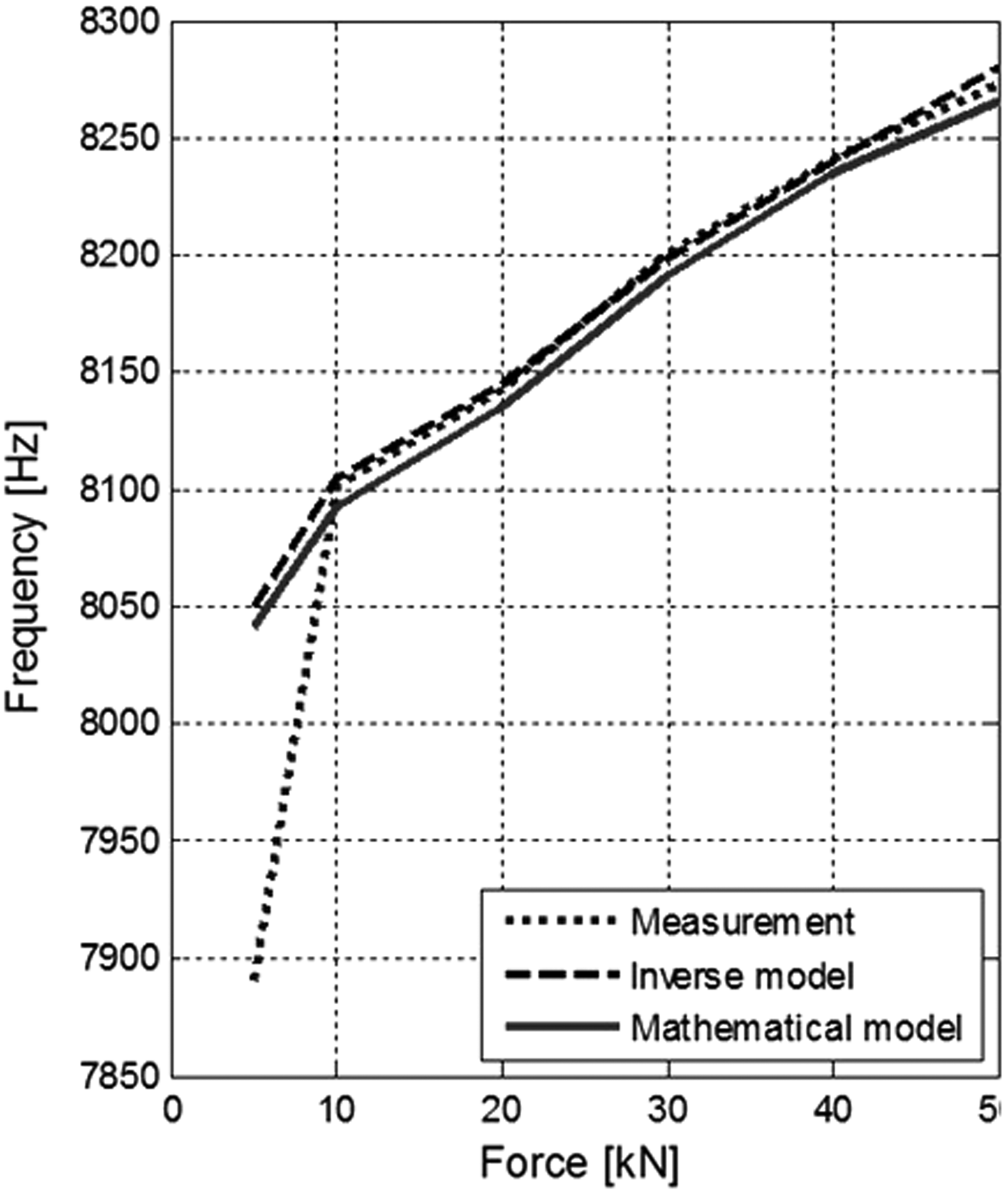
The comparison between measurement results and the model simulation.

Verification of simulation results

As mentioned before, the tests for metal section compressed with axial force in the range from 5 to 50 kN by applying the SAS were conducted in order to verify the derived models. The test results are presented in Table 3.

The simulation results generated by coupling a simple model of the executive system with the beam model, as well as the results from inverse model and beam model coupling, do not vary from the real object measurements. The results of the comparison are shown in Figure 16. When analyzing the plots, it can be noticed that the largest difference between simulation and real object measurement results occurs for the 5 kN load. It is due to the fact that the beam model assumed strictly defined beam vibration form, while the measurements were carried out for the beam, where the frequency shift had occurred. Therefore, it is important to protect the executive system with filters which prevents this phenomenon. A specific mode of beam oscillation was adopted for both the mathematical model and the identification. Wave velocity is in fact dependent on the oscillation form n. This velocity affects the delay between the emitter and the receiver in the SAS. Hence, the oscillation form n affects the resonant frequency of the SAS system. As part of research (15), it was discovered that the SAS system can “switch” by itself to use another form of oscillation with similar vibration amplitude. That is why model plots presented in Figure 16 are different from the actual measured frequency: at the load F = 5 kN, SAS system used a different form of oscillation than the assumed model. This effect is usually eliminated by applying band-pass filters which are built-in features in the receiver’s conditioner (Figure 1).

Conclusions

This paper presents the application of the SAS for the indirect stress change measurement in the axially compressed beam. Two models of the executive system were proposed. The first model was based on the identification of the sensor–conditioner–amplifier–emitter system. The second (mathematical) model was based on the equations for the electromechanical transducers, which were the piezoelectric sensor and the emitter. The model of the loaded beam, which determined the response at any point of the beam to the force applied to any other particular point of the beam, was also developed. Coupling the model of the executive system and the beam model allowed to underline the greatest advantage of the SAS system. Its application in the stress change measurements decreases significantly the requirements for the sampling frequency of the measurement system. The classic ultrasonic measurement systems so far require a signal sampling frequency of GHz to measure a very small wave TOFD change. The SAS system reduces this order to kHz. The frequency of the execution system was also measured. The TOFD for the wave passed through the tested material has, as always in case of the auto-oscillators, significant influence on its frequency. Therefore, the SAS measures indirectly the wave flight time, which alongside determines the construction stress state. This paper presents also the relation between this delay time and the stress of the sample under load.