This paper proposes a direction of arrival estimation based on sparse signal reconstruction in the presence of alpha noise by the off-grid orthogonal matching pursuit algorithm. Assuming Gaussian distribution as the noise model, the previous sparse reconstruction enhances robustness by utilizing the least square criterion-based direction of arrival estimation algorithms. However, they severely degrade, even invalid, when there is thick trailing and large impulse in the noise molded by stable distribution. In addition, due to the discretization of the potential angle space, the accuracy of these methods will be reduced when the target is not completely on the divided mesh exactly. Increasing the grid density to improve estimation effect will increase the computation burden. The compressed sensing signal model is reconstructed by reshaping the fractional lower order covariance matrix of the sensor array received signal. Based on the reshaped signal model, the novel reshaped orthogonal matching pursuit algorithm and reshaped off-grid orthogonal matching pursuit algorithm are derived. Compared to the least square criterion method with Gaussian distribution assumption, the proposed algorithm obtains high-resolution direction of arrival estimation in noise. Moreover, the reshaped off-grid orthogonal matching pursuit algorithm improves the direction of arrival estimation accuracy with off-grid target. Numerical simulation results demonstrate the effectiveness of proposed method in direction of arrival estimation with off-grid targets in noise.
Direction of arrival (DOA) estimation of multi-source signals is an important issue in the field of array signal processing, which is widely used in radar, sonar, wireless communications, and other fields. Many methods have been proposed in previous studies, but most of these methods are based on the assumption that the observed signal is mixed with additive noise, which takes Gaussian distribution as mathematical model. When the statistical properties of Gaussian noise are known, methods based on second-order moments and other algorithms based on the least square (LS) criterion can be used. These kinds of algorithms can effectively suppress Gaussian noise. The algorithm description is intuitive, and the process of calculation is simple.
Unfortunately, the assumption that the additive noise obeys Gaussian distribution is not universal, for there are plenty of other types of noise in nature, and impulsive noise is an important component of them. Research shows that impulsive noise is widely present in artificial audio environment, underwater environment, and various types of electromagnetic environments.1–3 Furthermore, in many applications, the non-Gaussian noises are expressed as stable distribution, such as electrical equipment and digital circuit switching noise, a variety of mechanical processing equipment’s electric spark noise, and the wireless communication harass signal noise. So signal processing technology under noise has practical significance. However, it is restricted in signal processing under noise because of the following properties:
There is no closed probability density function (PDF) of stable distribution, so the PDF-based algorithms are unavailable, such as maximum-likelihood method4 and Bayesian estimation algorithm.
Because there are no second-order moment and higher-order moment in stable distribution, and the second-order moment-based algorithm,5 high-order cumulant-based algorithm6 and the LS criterion-based algorithm cannot be used to deal with Gaussian noise.
In order to solve the above problems, the method of fractional low-order moment is proposed in Ma and Nikias.7 Due to the contribution of Ma and Nikias,7 the existing subspace-based algorithm, such as Multiple Signal Classification (MUSIC)8 and Signal Parameters via Rotational Invariance Techniques (ESPRIT),9 can be used in the presence of noise. In Zhong et al.,10 a novel DOA estimation method in impulsive noise is presented by applying particle filtering. In Zeng et al.,11 a -MUSIC algorithm robust to noise is proposed based on the norm criterion. The DOA estimation approach on spatial smoothing for coherent signals in impulsive noise is proposed in Li and Lin.12 However, the subspace-based algorithms are computationally expensive. For the last few years, many scholars have noticed the application of sparse reconstruction model in DOA estimation. Assuming the true DOAs exactly lie on the predefined grid points, though dividing the spatial angle with a predefined set of grid points densely enough, still not all is rational. So true DOAs of signal source in spatial angle are sparse, and sparse reconstruction technique to address DOA estimation problem can be adopted.
Sparse signal reconstruction, as one of the important research fields of Compressed Sensing (CS),13 attracts the attention of many scholars in the last decade. Several approaches are presented in articles. Original Sparse reconstruction model generates a norm optimization problem, which is a non-deterministic polynomial hard (NP-Hard) problem. An approach to avoid NP-Hard problem by converting the norm optimization to norm optimization is proposed in Donoho.14 It is a prominent contribution to provide a convex optimization approach for sparse reconstruction. But the norm optimization is a suboptimal approach, which approximates globally optimal solution, when it satisfies certain conditions. In Emadi et al.,15 orthogonal matching pursuit (OMP)-based DOA estimation is proposed as a solution to the norm optimization problem. In addition, sparse reconstruction with noise is another important topic. Based on the assumption of Gaussian noise, many approaches designed to enhance robustness are proposed (e.g. Basis Pursuit De-Noising (BPDN) algorithm16 and Danzig Selector algorithm17). Based on the assumption of noise, Zeng et al.18 devised a new definition of correlation called -correlation and developed -MP, weak -MP, and -OMP algorithms for robust sparse approximation. In Dai and So,19 an off-grid Bayes-optimal algorithm based on posterior probability is proposed for robust DOA estimation with noise.
Notably, the above methods do not preprocess the measured data to suppress noise. Although these algorithms can estimate targets in the presence of noise, it leads to reduced accuracy, when the signal-noise ratio (SNR) is at a lower level. In order to improve the accuracy, Ma et al.20 suppress Gaussian noise by second-order statistics and developed Khatri–Rao (KR) subspace approach, meanwhile Li et al.21 suppresses noise by fractional lower order statistics and reconstructed the CS signal model based on KR subspace approach. The convex optimization method, namely a suboptimal approach based on norm optimization, is used to solve the sparse reconstruction problem in Li et al.21
In this paper, the CS signal model is reconstructed by reshaping the fractional lower order covariance (FLOC) matrix based on KR subspace approach and devises two OMP algorithms, namely reshaped orthogonal matching pursuit (R-OMP) and reshaped off-grid orthogonal matching pursuit (R-OGOMP), to address DOA estimation problem with noise. Particularly, the R-OGOMP algorithm has three notable advantages. First, noise suppression performed by FLOC improves the accuracy when SNR is low. Second, OMP is an approach for norm optimization, which is a NP-Hard problem, superior to a suboptimal approach for norm optimization in precision. Third, off-grid framework formed by first-order Taylor expansion effectively deals with the targets, which are not exactly on the predefined grids without significant increase in calculations. In addition, to simplify the numerical calculation, the differential property of KR product is summarized and proved.
The symbols mentioned in the text are explained as follows: the indicates the absolute value of scalar; the indicates the norm of a vector; the superscripts , , and indicate transpose, conjugate, and conjugate transpose, respectively; the , , and indicate Hadamard product, Kronecker product, and KR product.
Stationary distribution
The PDF for the stable distribution does not have closed-form. Therefore, the stable distribution is usually represented by characteristic function as follows1
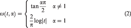
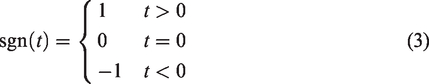
where
is the sign function
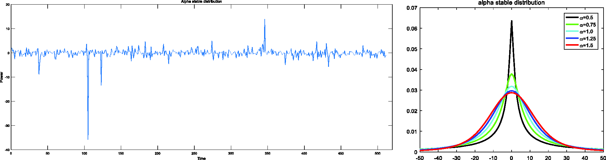
The important parameter in the equation is the characteristic exponent . The value of implies thickness in tails of distribution. The smaller the value, the greater the probability of random variables appearing far away from the center of the distribution, and the larger the noise impulse amplitude. When , the stable distribution has the same PDF as the PDF of Gaussian distribution; when , , the stable distribution performs the same statistical property as Cauchy distribution. So the stable distribution is considered as a generalized Gaussian distribution. Both Gaussian distribution and Cauchy distribution are particular cases of the family.
Figure 1 shows the time domain stochastic process in stable distribution and the probability distribution of stable distribution with different .
Stable distribution.
is the location parameter, which implies mean of the distribution when , or median when ; is the symmetry parameter; is the scale parameter, also called the dispersion. For study convenience, the standard symmetric distribution model of the stable distribution in signal processing is adopted. The standard symmetric distribution is defined by confirming , , , , and denoted by . The noise involved in the numerical simulation in this paper is modeled as .
An important property of the stable distribution is as follows
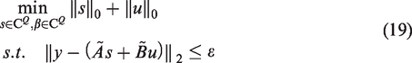
If , then
, when
, when
If , then
, for all
The consequence of the formulas above is that the second-order or higher moment of stable distributions tends to infinite, when . Accordingly, the second-order moment method and high-order cumulant method widely used to suppress Gaussian noise are invalid in noise. The LS criterion method of sparse signal reconstruction in CS is invalid all the same in noise.
Compressed sensing
The main research directions of CS are as follows
1. Sparse signal compression acquisition
The technology or equipment compresses high-dimensional sparse signals into low-dimensional non-sparse signals during the acquisition process directly.
2. The over-complete dictionary structure
The methods construct a matrix with columns larger than rows according to the principle of CS.
3. Sparse signal reconstruction
The approaches reconstruct high-dimensional signals from low-dimensional received signals and determine non-zero elements and their values.
In this paper, the sparse signal reconstruction algorithms are mainly used to realize DOA estimation. The sparse reconstruction mathematical model is expressed as
where is received vector; () is a matrix that obeys a condition known as RIP,13 we name it measurement matrix; is input vector. Sparse reconstruction is a problem try to reconstruct the higher-dimensional vector from the lower-dimensional vector under the condition that and are known. From the point of view of solving mathematical equation, this is an under-determined system, which cannot be solved. But when the sparse conditions are satisfied, formula (5) converts to a solvable constrained optimization problem
In the presence of noise, the formula is reformulated as
However, norm optimization is the NP-Hard problem. To solve the problem, scholars suggest an effective solution named greedy algorithm. The OMP algorithm is the most typical method.
DOA estimation based on FLOC matrix reconstruction
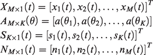
Consider the case that there are K narrow-band far-field signal sources , in the spatial with different DOAs , arriving at a uniform linear array (ULA) with M sensors. The received signals of each array element have additive noise , , , . Without loss of generality, the noise satisfies the assumption that it is independent identically distributed and uncorrelated to the signal. The received signal vector of the array can be expressed as
where
where , is the output value of the array element; , is the steering vector, which can be expressed as
where, is the carrier signal wavelength; is the intersensor spacing.
If the noise item in formula (8) is noise and the characteristic exponent , then the FLOC matrix can be expressed as21
where, is the steering matrix in formula (8); is a diagonal matrix; the elements of main diagonal can be treated as the fractional low-order power of the signal source; can be treated as the power level of the additive noise and denotes the identity matrix; is the eigenvalues obtained by eigenvalue decomposition of FLOC matrix ; so the item can be treated as a known vector.
The element of matrix can be defined as
where, denotes the fractional lower order exponent, which satisfies and guarantees is bounded. When , the formula (10) is consistent with the covariance matrix in Gaussian noise. Move the item to the left-hand side of formula (10), and then
Where
Applying the vectorization operator in Ma et al.20 on formula (10), it is reshaped into CS form as follows
where, represents the expansion of a matrix by columns into a vector; is the KR product reshaped matrix, which is expressed as
where, is reshaped matrix and is equivalent source vector. Formula (13) is reformulated as
where
Define a set obtained by meshing the spatial angle; the number of the predefined set of grid should be greater than the number of the signal sources and the row number of reshaped matrix; define is the over complete dictionary; can be interpreted as the steering vector of the virtual array; can be interpreted as the sparse signal source power vector in spatial which contains nonzero elements; the nonzero element equals to , and the predefined angle equals to DOA of the signal source ,; the nonzero element index of vector is the position index of the sequence of spatial angles and the nonzero element value is the power of the signal source.
From the above definition, the sparse can be formulated as
Through contrast, formulas (16) and (5) have the similar sparse structure and the DOA estimation problem can be addressed by applying the algorithms of sparse reconstruction. The problem is converted into the -norm optimization and expressed as
OMP algorithm can be utilized to solve the -norm optimization. Thus, the DOA of the target signal source is determined according to the nonzero elements index of the vector .
R-OMP algorithm
The basic idea of OMP algorithm is to treat the observation vector as a linear combination of the basis of the overcomplete dictionary matrix. The nonzero elements in the sparse vector are the coefficients of the basis. The zero elements in the sparse vector mean that the coefficient of the basis is zero, so the vectors in the overcomplete dictionary corresponding to the zero elements have no contributions to the linear combination of the observation vector. Therefore, sparse reconstruction problem can be addressed as long as the basis and corresponding coefficients that contribute the most to the linear combination are found. In OMP algorithm, the contributions of vectors of overcomplete dictionary in the linear combination is determined by calculating the correlation coefficient between the observation vector and the vector of overcomplete dictionary. The vectors of the overcomplete dictionary of the first ones with the largest contribution are regarded as the basis. The position of its nonzero coefficient in sparse vector can be determined by the index of the basis. The value of the coefficient can be obtained by iterative calculation of residuals. In the process of numerical calculation, the correlation coefficient is transformed into the inner product of the observation vector and the overcomplete dictionary vector under the background of Gaussian noise. The algorithm needs to satisfy several preconditions:
The target number is known.
The inner product operation can be performed between the observed vector and overcomplete dictionary vector.
The target DOA falls exactly on the predefined grid.
The sparse reconstruction problem is addressed based on the reshaped model referred to formula (17) through OMP algorithm and name it R-OMP. The steps of R-OMP algorithm are summarized in Algorithm 1.
Outputs: The sparse signal and the residue error vector .
R-OGOMP algorithm
R-OMP algorithm mentioned in section “R-OMP Algorithm” requires that the target DOAs exactly fall on the divided grids before DOA can be accurately estimated by sparse reconstruction. Unfortunately, the target has a high probability of not falling on the grids actually. It reduces the estimation accuracy because of grid mismatch.
Therefore, a novel off-grid OMP algorithm is proposed based on FLOC matrix reconstruction named R-OGOMP. The algorithm realizes DOA estimation based on sparse reconstruction in noise. And it also improves the estimation accuracy by utilizing off-gird approach. The basic idea is expounded as follows.
The first-order Taylor series expansion for in formula (16) is performed22,23
where, is virtual steering matrix in formula (16); is mismatch matrix obtained by taking the partial derivative of about ; denotes the mismatch deviation vector where ; denotes the true DOA; and is diagonal matrix operation. According to the literature,24, and have the same sparse structure. So formula (18) is converted into the optimization problem
As long as the sparse structure of the vector is determined, the mismatch deviation vector has the same sparse structure. Inspired by Zeng et al.11 and Liu et al.22, we apply alternating direction iterative method to obtain and . The mathematical model is expressed as followse
where, is the sparse construction estimation value of in the iteration; and is the estimation value of . Through addressing the problem of formulas (20) and (21), the sparse signal and can be obtained. And can be obtained by utilizing the nonzero elements of to solve the problem for any . Then update the following iteration operators
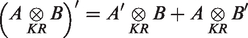
Because is given by the KR product, its matrix structure is complex. It is more complex to calculate the partial derivatives of matrix directly, because it takes up more computing resources and slows down computing time. The differential property of KR product is presented and proved.
Property 1: For an arbitrary matrix , , , , and matrix , , , , there is
where, denotes differential operation; both and are the function matrix of the parameter .
: and is the function vector of parameter in and B respectively.
The efficiency of matrix operation is improved by applying Property 1. in formula (18) derived from property 1 expresses as
With the analysis above, the steps of R-OGOMP algorithm is summarized in Algorithm 2.
Outputs: The sparse signal and , estimation of angle .
Then discuss the stopping criteria:
Stop the iteration steps after a fixed number , i.e. .
Run until the norm of the residual declines to a level . That is, .
Halt the algorithm when residual error rate drops below a threshold.
Numerical simulations
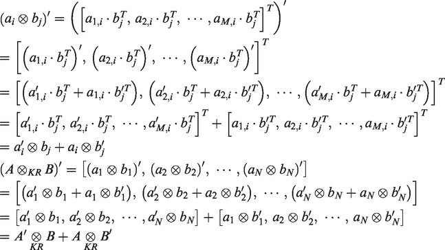
In this section, some numerical experiments are provided to assess the performance of the R-OMP and R-OGOMP algorithms. The stable distribution is taken to model the noise. The general signal-to-noise ratio (GSNR) is defined as
where, is the scale parameter of noise; is the snapshots; and is the sampling values of the signal sources. The mean square error(MSE) of the DOAs estimation is defined as
where is the number of target DOAs; is the DOA estimation on the snapshot; and is the true DOA.
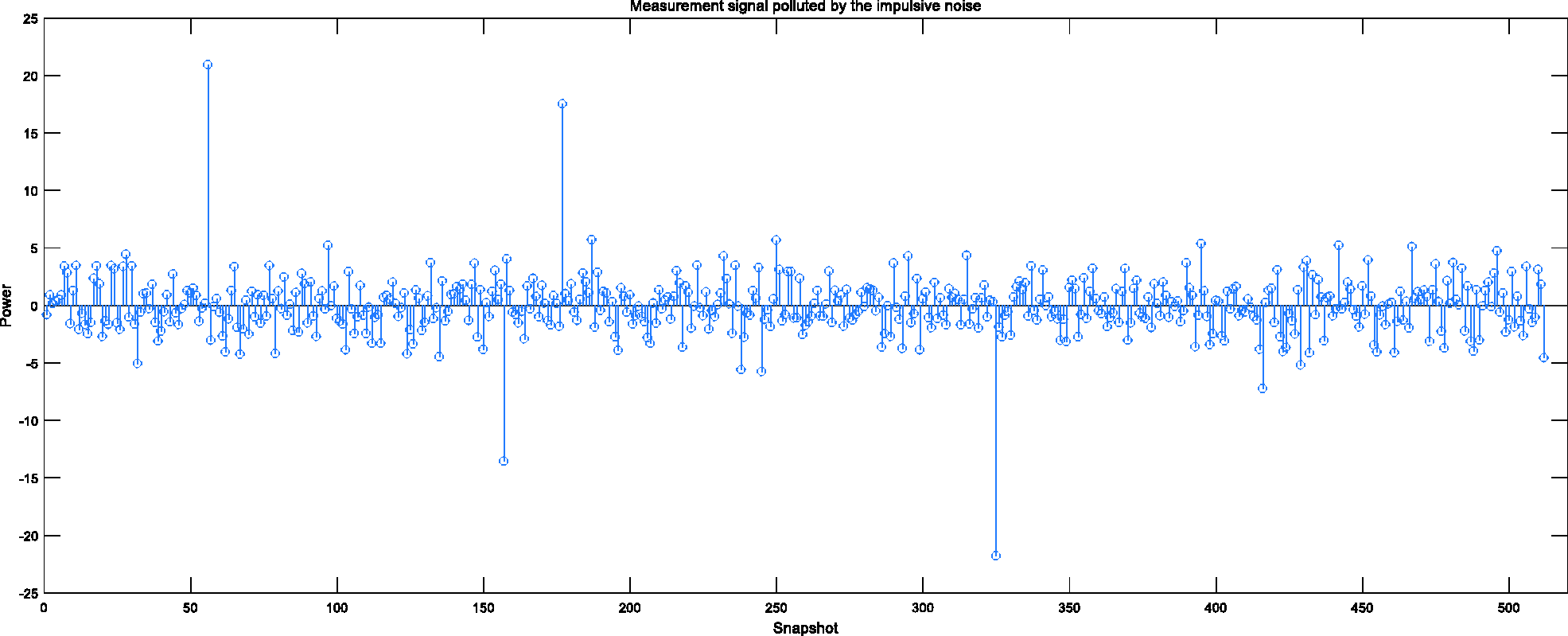
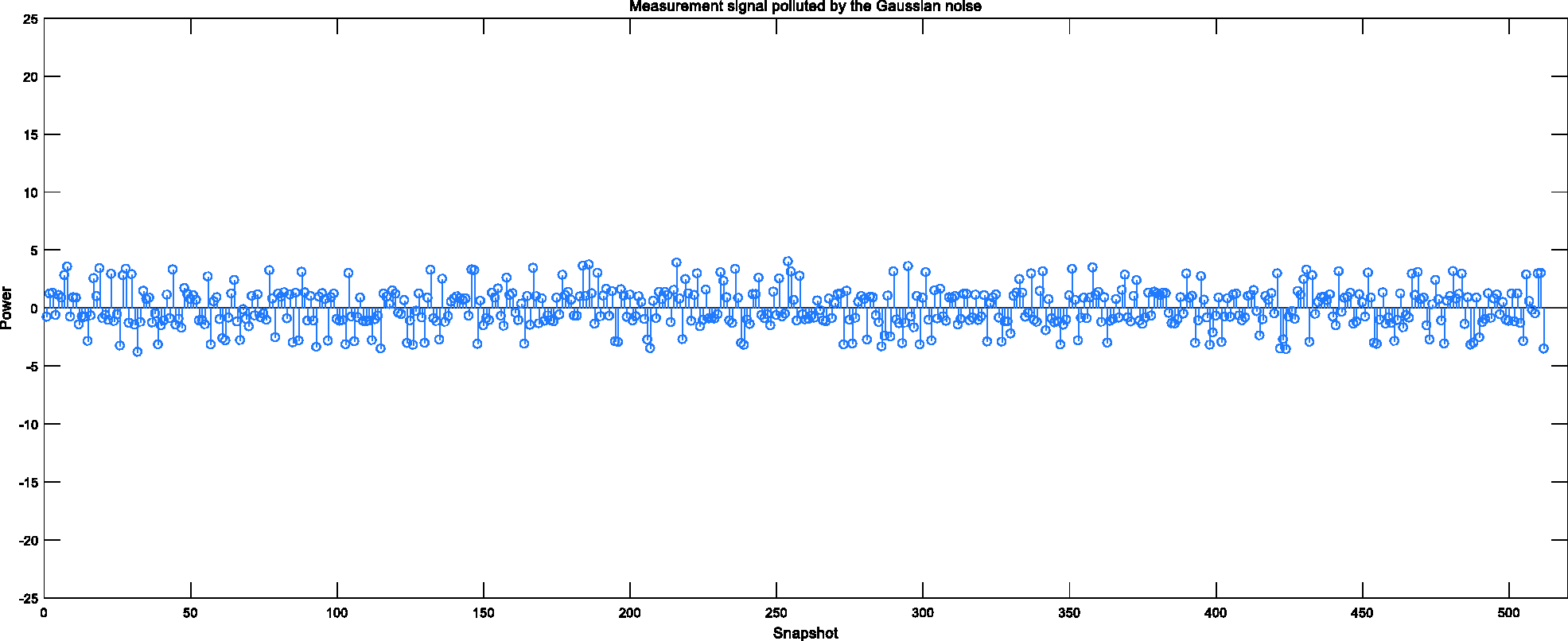
Figure 2 shows the measurement signal polluted by the impulsive noise and Figure 3 shows the measurement signal polluted by the Gaussian noise. It can be observed that the measurement signal in Figure 2 contains more impulse compared with Figure 3.
Measurement signal polluted by the impulsive noise.
Measurement signal polluted by the Gaussian noise.
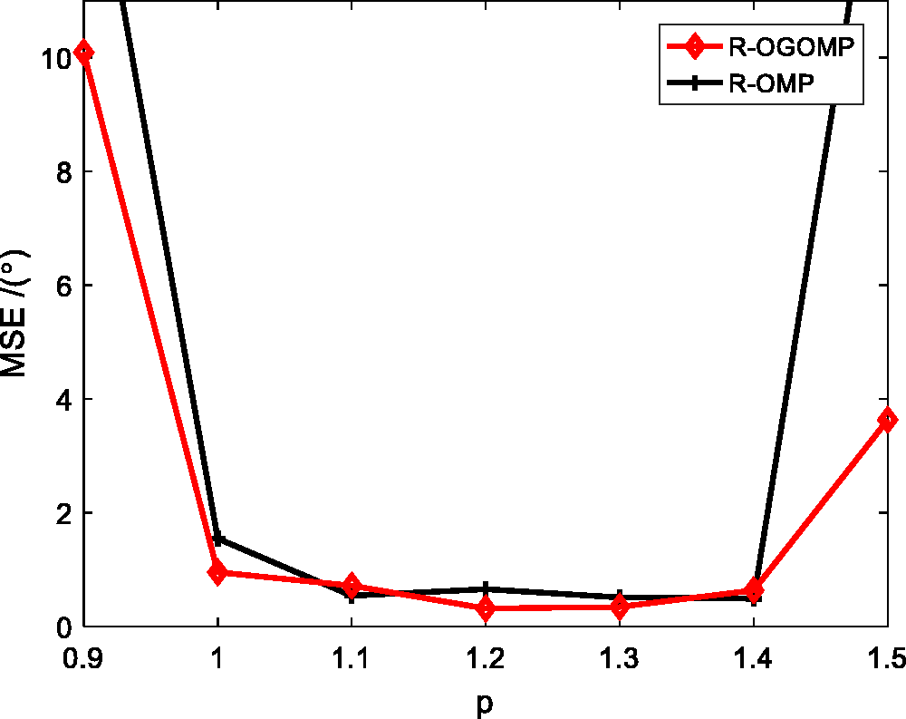
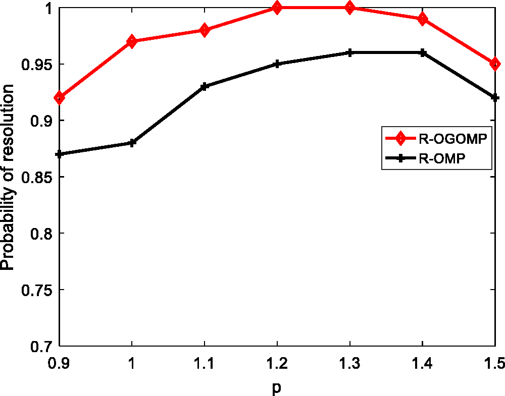
Determination of the value of p
To determine the value of p, we design two simulations experiments to observe the effect on accuracy and success probability when the p value changes. First, Shao and Nikias1 point out that the definition of FLOC is valid when . Second, we consider the noise in the following simulations is noise with the characteristic exponent . So, p value should be taken in intervals .
The assumption of the experiment is that the numbers of sensors in the array and the snapshots are and , respectively. The intersensor spacing is half a wavelength. The DOAs of two spatial signal sources () are picked at random in the interval and . The numbers of Monte Carlo trials are . The characteristic exponent and . For R-OGOMP algorithm, the predefined angle is .
Figure 4 shows that the performance of proposed algorithms on accuracy has not changed much when p value is 1.1, 1.2, 1.3, and 1.4. Figure 5 shows that the success probability of proposed algorithms is higher when p value is 1.2 and 1.3. Comprehensive consideration, we take as the default parameters in the following simulations.
MSE of DOA estimation of two signal sources in noise with versus p.
Success probability of DOA estimation of two signal sources in noise with a = 1.5 versus p.
Multiple source DOA estimation in α noise
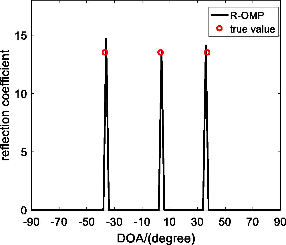
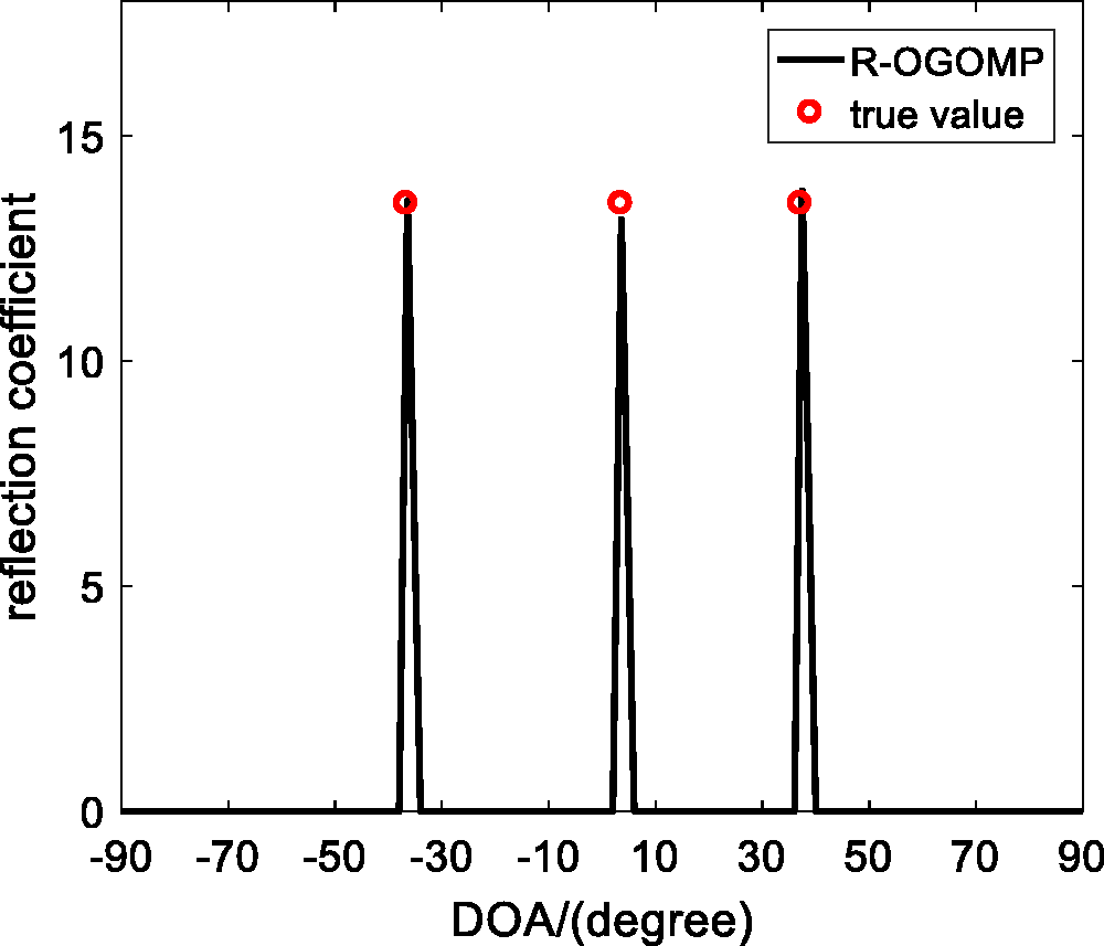
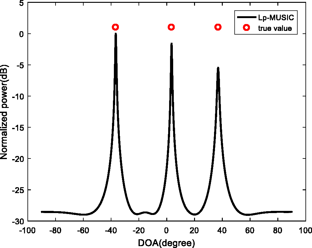
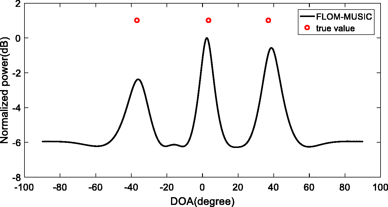
In the simulation, the effectiveness of proposed algorithms in noise is demonstrated, and the resolution is compared. There are three signal sources in spatial and the DOAs, of them are . The number of the sensors in the ULA is , and the intersensor spacing is half a wavelength. The snapshots are . For R-OGOMP algorithm, the predefined grid angle is . The noise is noise with the characteristic exponent and . We take for FLOC-based methods. Figures 6to 9 show the spatial spectra of four independent trials, respectively. Figures 6 and 7 show that the R-OMP and R-OGOMP algorithms can realize DOA estimation based on sparse reconstruction in noise. The spatial spectrums in Figures 6 and 7 are sharper than those in Figures 8 and 9. It demonstrates that the proposed methods in this paper have higher resolution than -MUSIC and FLOM-MUSIC algorithms.
Normalized spatial spectrum of R-OMP algorithm is noise with and . The red circles show the true value of DOAs.
Normalized spatial spectrum of R-OGOMP algorithm is noise with and . The off-grid angle is . The red circles show the true value of DOAs.
Normalized spatial spectrum of -MUSIC algorithm is noise with and . The step-size is 0.1.
Normalized spatial spectrum of FLOM-MUSIC algorithm is noise with and . The step-size is 0.1.
Estimation accuracy comparison
Monte Carlo experiments are carried out to compare the performance of the proposed algorithms with MMV-OMP, FLOM-MUSIC, and -MUSIC algorithms on the accuracy. The numbers of sensors in the array and the snapshots are and , respectively. The intersensor spacing is half a wavelength. The DOAs of two spatial signal sources () are picked at random in the interval and . is taken for R-OGOMP, Fractional Lower Order Moment-MUSIC(FLOM-MUSIC), and -MUSIC algorithms. The numbers of Monte Carlo trials are .
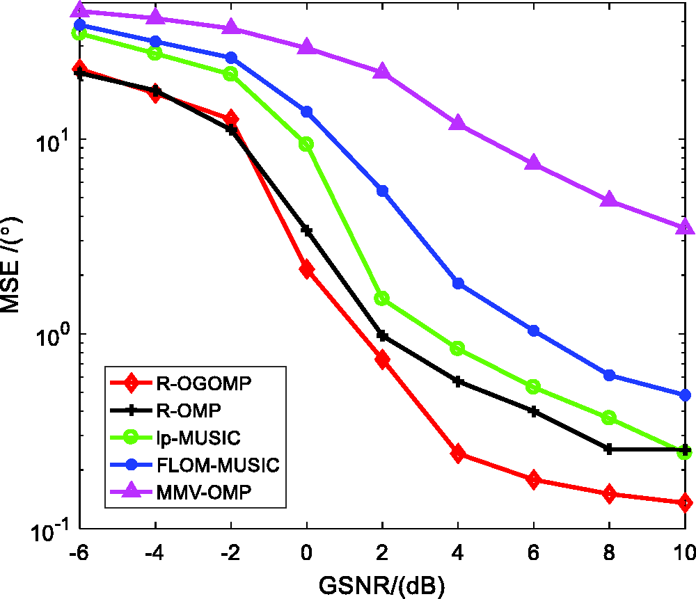
Figure 10 illustrates the MSE of the five methods decreases with the increase of GSNR. The characteristic exponent of noise is . For R-OGOMP algorithm, the predefined angle is . It can be seen that the conventional sparse reconstruction-based DOA estimation method named Multiple Measurement Vector-OMP (MMV-OMP) algorithm is not robust in noise. FLOM-MUSIC and -MUSIC algorithms have an improved performance. R-OMP and R-OGOMP algorithms have the best performance compared with other methods in most cases. The R-OGOMP algorithm is superior to R-OMP algorithm, especially when .
MSE of DOA estimation of two signal sources in noise with versus GSNR.
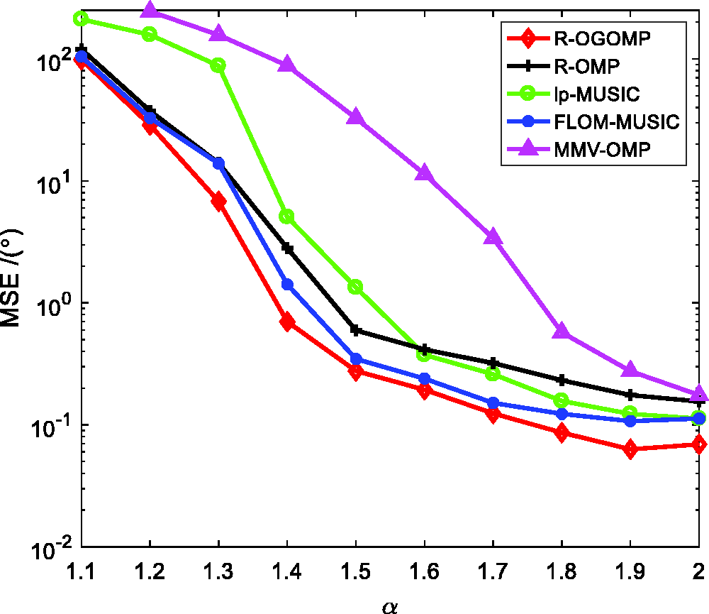
Figure 11 shows the trend of MSE of the five methods versus . The predefined angle of MMV-OMP, R-OMP, and R-OGOMP algorithms is , meanwhile the step size of FLOM-MUSIC and -MUSIC algorithms is . The GSNR is 5 dB. It shows that the MSE decreases with the increase of and the R-OGOMP algorithm has the best performance on estimation accuracy. The estimation accuracy of MMV-OMP algorithm is lower than other four algorithms. The reason is the MMV-OMP is not robust in noise. The performance of FLOM-MUSIC algorithm is better than R-OMP algorithm. When , the noise model converts to Gaussian noise and the performance on accuracy of all the five algorithms is similar.
MSE of DOA estimation of two signal sources in noise versus at .
Success probability comparison
In this section, the Monte Carlo experiments are performed to compare the success probability of MMV-OMP, R-OMP, R-OGOMP, FLOM-MUSIC, and -MUSIC algorithms. The assumption of the experiment is that , , ,, , and . It can be defined the numerical simulation is success, when the DOA estimated deviation sum of two signal sources is less than 1°.
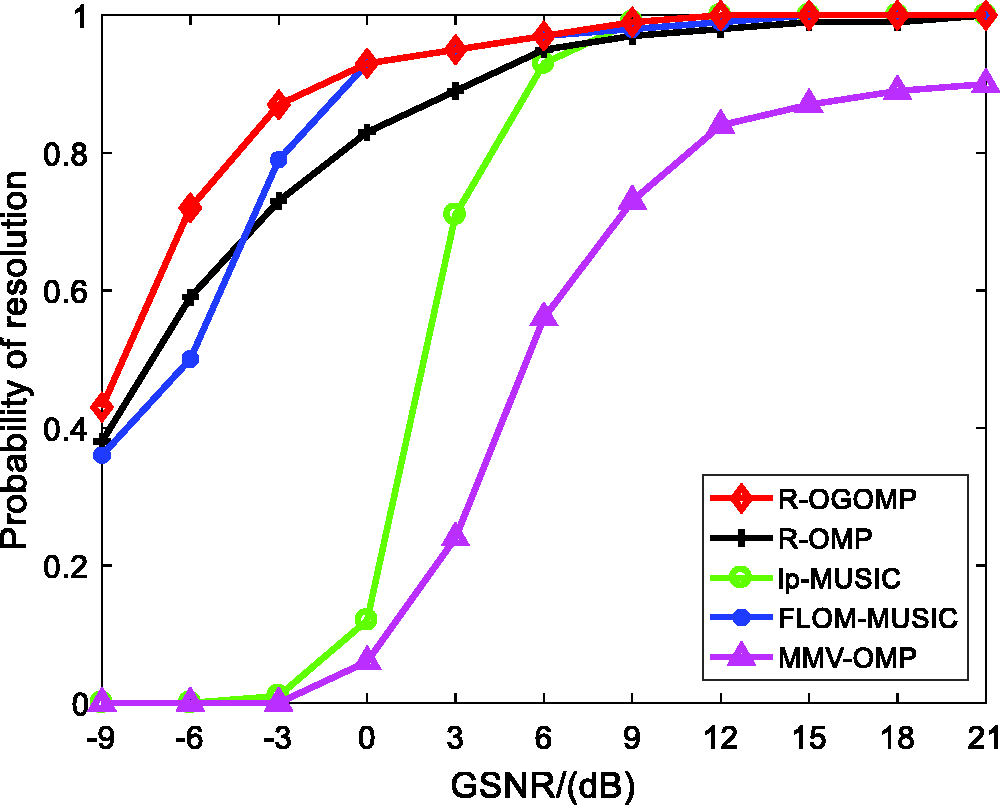
Figure 12 shows the trend of success probability versus GSNR. Make and . The numerical results indicate conclusions as follows:
Success probability of DOA estimation of two signal sources in noise with versus GSNR.
The MMV-OMP algorithm is not robust in noise, so its success probability is the lowest at different GSNR. Without noise suppression, the success probability of the MMV-OMP algorithm is zero when . Because of the noise suppression, R-OGOMP, R-OMP, and FLOM-MUSIC algorithms have high success probability even when . The performance of R-OGOMP algorithm on success probability is the best, especially when .
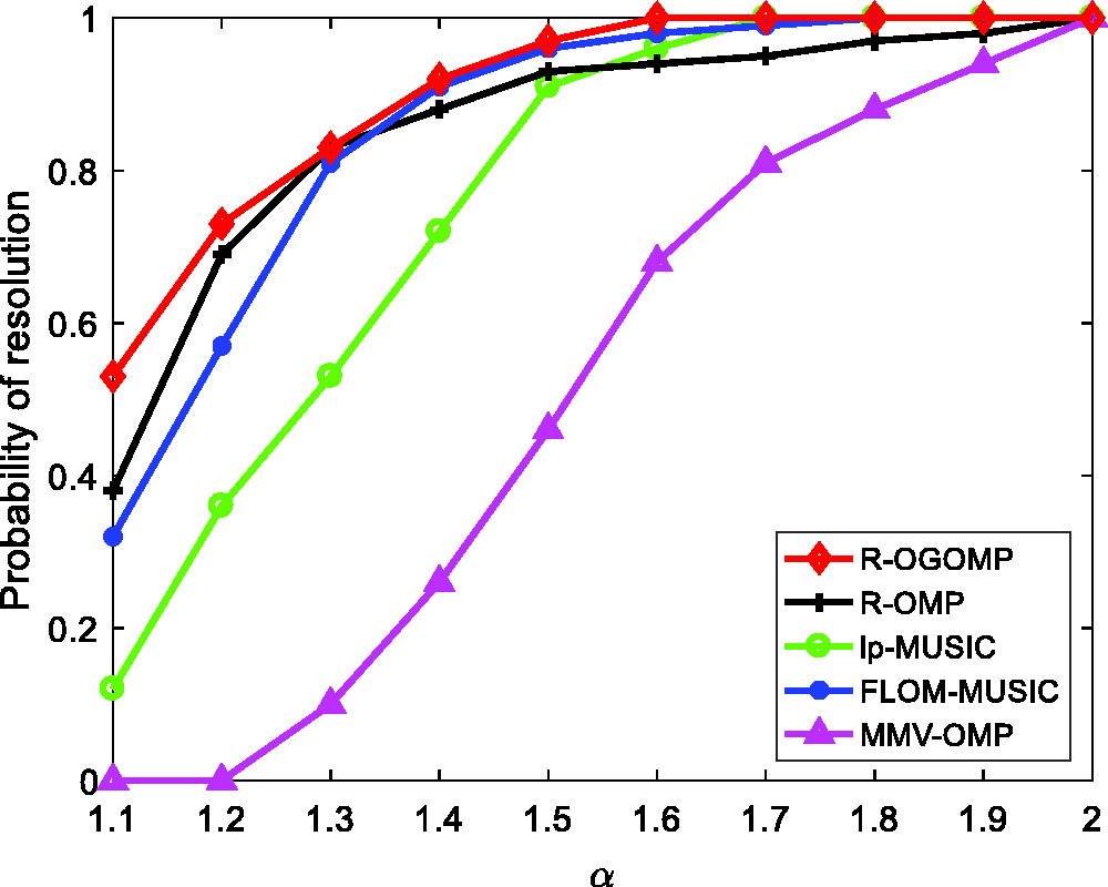
Figure 13 shows the trend of success probability versus . Make and . The result indicates that the performance of R-OGOMP algorithm is the best and the success probability is 1 when . When , the performance of the five algorithms is similar.
Success probability of DOA estimation of two signal sources in noise versus at .
Off-grid performance comparison
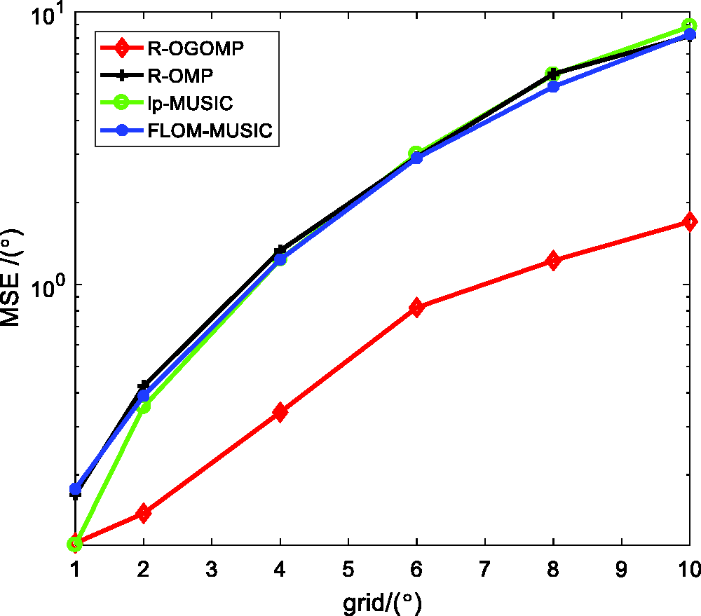
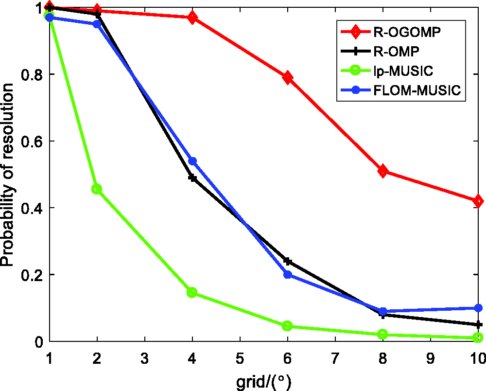
The statistical performance of R-OGOMP, R-OMP, FLOM-MUSIC, and -MUSIC algorithms on different predefined grid angles is compared in this section. The assumption of the experiment is that , , , , , and . It can be defined success, when sum of DOA estimation deviation is < 1°. The predefined grid angle is equivalent to step size of -MUSIC and FLOM-MUSIC algorithms.
Figure 14 shows that the MSE of R-OGOMP algorithm is significantly better than other algorithms as the predefined grid angle increases.
MSE of DOA estimation of two signal sources in noise with and at Versus .
Figure 15 shows that the algorithm with highest success probability versus increasing predefined grid angle is R-OGOMP. The lowest one is -MUSIC algorithm.
Success probability of DOA estimation of two signal sources in noise with and at versus .
Conclusion
This paper proposes a new array manifold by reshaped FLOC matrix and the off-grid model is introduced. The DOA estimation problem is addressed by OMP algorithm based on sparse reconstruction of the reshaped vector, which are named R-OMP and R-OGOMP algorithms. Different from robust-based algorithms, accuracy performance is improved by noise suppression. Because of the off-grid model, the accuracy of DOA estimation is improved when there are off-grid targets in spatial and the number of predefine grid is reduced. In the numerical calculation, the differential property of KR product is summarized to reduce computational complexity and proved. Simulations results demonstrate that the proposed algorithm realizes DOA estimation in presence of noise. The R-OGOMP algorithm outperforms several existing DOA estimation methods in terms of estimation accuracy and probability of resolution.
Footnotes
Declaration of conflicting interests
The author(s) declared no potential conflicts of interest with respect to the research, authorship, and/or publication of this article.
Funding
The author(s) received no financial support for the research, authorship, and/or publication of this article.
ORCID iD
YiRan Shi
References
1.
ShaoMNikiasCL.Signal processing with fractional lower order moments: stable processes and their applications. Proc IEEE1993;
81: 986–1010.
2.
SocheleauFXPastorDDuretM.On symmetric alpha-stable noise after short-time Fourier transformation. IEEE Signal Process Lett2013;
20: 455–458.
3.
LuoJWangSZhangE.Signal detection based on a decreasing exponential function in alpha-stable distributed noise. KSII Trans Internet Inf Syst2018;
12: 269–286.
4.
TsakalidesPNikiasCL.Maximum likelihood localization of sources in noise modeled as a Cauchy process. IEEE Trans Signal Process1995;
43: 2700–2713.
5.
ValletPMestreXLoubatonP.Performance analysis of an improved MUSIC DoA estimator. IEEE Trans Signal Process2015;
63: 6407–6422.
6.
HouCLWangDS. The Fourth Order Cumulant-Based MUSIC Algorithm for Harmonic Retrieval in Colored Noise. In: Wri international conference on communications & mobile computing, Kunming, China, 6-8 January 2009.
7.
MaXNikiasCL.Joint estimation of time delay and frequency delay in impulsive noise using fractional lower order statistics. IEEE Trans Signal Process1996;
44: 2669–2687.
8.
TsakalidesPNikiasCL.The robust covariation-based MUSIC (ROC-MUSIC) algorithm for bearing estimation in impulsive noise environments. IEEE Trans Signal Process2002;
44: 1623–1633.
9.
ZhangJQiuT.The fractional lower order moments based ESPRIT algorithm for noncircular signals in impulsive noise environments. Wireless Pers Commun2017;
96: 1673–1690.
10.
ZhongXPremkumarABMadhukumarAS.Particle filtering for acoustic source tracking in impulsive noise with alpha-stable process. IEEE Sensors J2013;
13: 589–600.
11.
ZengWJSoHCLeiH.Lp-MUSIC: robust direction-of-arrival estimator for impulsive noise environments. IEEE Trans Signal Process2013;
61: 4296–4308.
12.
LiSLinB. On spatial smoothing for direction-of-arrival estimation of coherent signals in impulsive noise. In: Advanced information technology, electronic & automation control conference, Chongqing, China, 19-20 December 2015.
13.
CandèsEJ.The restricted isometry property and its implications for compressed sensing. C R Math2008;
346: 589–592.
14.
DonohoDL.For most large underdetermined systems of linear equations the minimal L1-norm solution is also the sparsest solution. Comm Pure Appl Math2006;
59: 907–934.
15.
EmadiMMiandjiEUngerJ.OMP-based DOA estimation performance analysis. Digital Signal Process2018;
79: 57–65.
16.
ChenSSaundersMADonohoDL.Atomic decomposition by basis pursuit. Siam Rev2001;
43: 129–159.
17.
CandesETaoT.The Danzig selector: statistical estimation when p is much larger than n.Ann Stat2005;
35: 2313–2351.
18.
ZengWJSoHCJiangX.Outlier-robust greedy pursuit algorithms in Lp-space for sparse approximation. IEEE Trans Signal Process2015;
64: 60–75.
19.
DaiJSoHC.Sparse Bayesian learning approach for outlier-resistant direction-of-arrival estimation. IEEE Trans Signal Process2018;
66: 744–756.
20.
MaWKHsiehTHChiCY.DOA estimation of quasi-stationary signals with less sensors than sources and unknown spatial noise covariance: a Khatri–Rao subspace approach. IEEE Trans Signal Process2010;
58: 2168–2180.
21.
LiSHeRLinB, et al.
DOA estimation based on sparse representation of the fractional lower order statistics in impulsive noise. IEEE/CAA J Autom Sinica2018;
5: 860–868.
22.
LiuQ-YZhangQLuoY, et al.
Fast algorithm for sparse signal reconstruction based on off-grid model. IET Radar Sonar Navig2018;
12: 390–397.
23.
ZhouCGuYShiZ, et al.Off-grid direction-of-arrival estimation using coprime array interpolation. IEEE Signal Process Lett2018;
25: 1710–1714.
24.
YangZZhangCXieL. Stable signal recovery in compressed sensing with a structured matrix perturbation. In: 2012 IEEE international conference on, Acoustics, speech and signal processing (ICASSP), Kyoto, Japan, 25-30 March 2012.