
Abstract
In order to extract fault impulse feature of large-scale rotating machinery from strong background noise, a sparse feature extraction method based on sparse decomposition combined multiresolution generalized S transform is proposed in this paper. In this method, multiresolution generalized S transform is employed to find the optimal atom for every iteration, which firstly takes in to account the generalized S transform with discretized adjustment factors, then builds an atom corresponding to the maximum energy. The multiresolution generalized S transform has better accuracy compared to generalized S transform and faster searching speed compared to the orthogonal matching pursuit method in selecting the optimal atom. Then, the orthogonal matching pursuit method is used to decompose the signal into several optimal atoms. The proposed method is applied to analyze the simulated signal and vibration signals collected from experimental failure rolling bearings. The results prove that the proposed method has better performances such as high precision and fast decomposition speed than the traditional orthogonal matching pursuit method method and local mean decomposition method.
Introduction
Vibration signals of rotating machinery can be divided into two major categories, one is signals with shaft rotation frequency and its harmonics caused by faults such as misalignment and imbalance, and the other are signals with modulation components caused by faults such as crack, pitting, and spalling. 1 In this paper, the proposed method is mainly aimed at extracting these modulation signals, which present characteristics of sparsity, weakness, and aperiodicity. 2
The traditional fast Fourier transform (FFT) is effective in extracting of feature frequency from signals with shaft rotation frequency and its harmonics, but it is limited to extracting local feature from modulation signals.3–5 Methods such as generalized S transform (GST), wavelet transform (WT), empirical mode decomposition (EMD), local mean decomposition (LMD) are widely applied in the mechanical fault diagnosis to extract local features.6–10 GST makes the width of window vary with the frequency, which is adoptable for analyzing modulation fault signals because it can adjust its time–frequency resolution effectively. Ma and Jiang11 proposed a modified window design method for S transform to improve the time–frequency localization, which can generate windows with different width profiles for multicomponent signals through selecting proper tuning parameters of a sigmoid function. Cai and Li12 introduced a time–frequency domain denoising method using the GST, in which a time–frequency filter factor is constructed to filter the vibration signal in the time–frequency domain, and can eliminate strong noise and can be used to extract the edge band structure that reflects the fault mode of gear. 12 But GST is invalid to decompose complex signal into simple components. To solve this problem, Huang et al.13 presented EMD to decompose arbitrary signals into a set of intrinsic mode functions (IMFs), which can be regarded as the basis functions derived from the nature of signals. To improve the end effects and mode mixing of EMD, Liu et al.14 provided a hybrid fault diagnosis method based on the second generation wavelet denoising and the LMD, which has better performances such as high signal-to-noise ratio (SNR) and fast convergence speed, and Wang et al.15 provided the time–frequency analysis based on ensemble LMD and fast kurtogram, which can be applied to rolling bearing. However, these methods are invalid in weak and sparse impulse extraction from low-SNR fault signals because of nonoptimal decomposition levels, end effects, and mode mixing.16–18
To solve this problem, Mallat and Zhang19 introduced a sparse representation method, in which the redundant dictionary is constructed through quantized mathematical model of fault signals. As the over–complete dictionary is constructed based on the time–frequency characteristic of the fault signals, fault impulses can be represented with a linear combination of several atoms simply and adaptively. Many methods appeared to get a set of optimal atoms to express the fault signals, such as matching pursuit (MP), orthogonal matching pursuit (OMP), and stagewise orthogonal matching pursuit (StOMP).20–23 Sparse representation can be divided into two major classes: atomic decomposition algorithms and dictionary learning methods. Wang et al.24 proposed a fault diagnosis method for weak fault of rolling bearing based on minimum entropy deconvolution and sparse decomposition, which was more effective in weak fault feature extraction compared to WT. Yan and Zhou25 proposed a coherent cumulant StOMP method to implement fast sparse representation for weak fault. Zhang et al.26 proposed a whale optimization algorithm (WOA)-optimized OMP with a combined time–frequency atom dictionary, which can optimize the atom parameters for best approximating the original signal with the dictionary atoms.
Although these sparse representations can identify the impulse fault accurately, there have been insufficient in algorithm complexity and computational efficiency. 27 Inheriting the ability of the time–frequency location of GST, this paper proposes a sparse feature extraction method based on sparse decomposition combined multiresolution generalized S transform (SD–MGST) to extract the impulse fault feature. This method is based on OMP, and the MGST is employed to find the optimal atom in each iteration, which simplifies the inner product of matching pursuit in sparse decomposition and ensures that the time–frequency factors of selected atom are optimal in each iteration.
Sparse decomposition and generalized S transform
Feature of pulsing fault signals
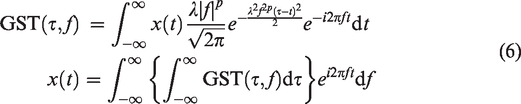
Bearings are critical components in rotating machinery, temperature change, material mixtion, stress variation, and chemical corrosion usually cause damage fault such as cracking, pitting, and spalling. And these failures would generate damping vibration caused by the striking between rolling elements and inner ring or outer ring. These damping vibration signals can be described by Gabor time–frequency signal as follows
Sparse decomposition
Traditional signal representation methods are based on complete bases, such as FFTs and WTs. These methods can get the only representation of signal. Yet, for signals carrying local feature, they would be invalid to get a simplified representation caused by excessive decomposition. In order to get sparse expression for these signals, Mallat provided a novel representation method based on an over-complete dictionary, which can get the sparsest representation with least atoms from the dictionary to represent the signals. 14
Let the set D = {gi|i = 1, 2, … , M}, where ǁgiǁ = 1, the length of gi is N, and card(D) ≫ N. D can be called over-complete dictionary. To represent any function f, we must select several optimal atoms from dictionary D, so that the sparse representation of f can be written as

The approximate error σ = ǁ f – fkǁ, so in the least approximation error condition, selecting the sparsest atoms to approximate the signal is equivalent solving the problem of 0-norm
To solve this NP-hard problem, many sparse decomposition algorithms have appeared, such as MP, OMP, BP, StOMP. And OMP is the most widely used method with the advantages of computation complexity, convergence rate, and approximation accuracy. 16
Compared to MP, the improvement of OMP is that all the selected atoms should be orthogonalized in each iteration to avoid selecting atoms repeatedly. So at the same accuracy, OMP has faster convergence rate than MP, and can get the optimal solution.
The main algorithm flow of OMP is shown as follows.
Step 1: Construct redundant dictionary
Step 2: Set residual
Step 3: Compute the correlation of observed signal and atoms in dictionary
Step 4: Select the most relevant atom γi = argγmax|
Step 5: Update the index set in the library of selected atoms Γ i = Γ i ∪ γi;
Step 6: Update coefficient
Step 7: Update residual
Step 8: Update number of iteration i = i + 1;
Step 9: Decide whether to stop, if stop, k = i – 1; if not, return step 3;
Step 10: Get the representation of
Finally, the sparse expression of

It is easy to prove
These indicate that the optimal atoms extracted each time will not overlap with the atoms previously extracted. This advantage makes the OMP to have obvious performance on the convergence rate and sparseness than MP. 29
The algorithm complexity and computational efficiency of OMP is determined directly by the pursuit of optimal atom in step 3 and step 4. The general strategy of optimal atom pursuit is according to the largest inner product. So, OMP also faces the problem of how to get the fast matching speed.
Generalized S transform
The classical FFT lacks the variable time–frequency resolution to analyze the time–frequency characteristic for modulation fault signals. Although the short-time Fourier transform (STFT) alleviated this shortcoming, it is still difficult to be widely applied to modulation fault signals with multiple frequencies due to the fixed windows.
To improve the time–frequency resolution, GST makes the width of window vary with the frequency, so that it processes multiresolution characteristic. The transform and the inverse transform of GST is defined as follows
According to Heisenberg uncertainty principle, the window should be narrower to get higher time resolution, and wider to get higher frequency resolution. 31
The window size of GST is determined by both the adjustment factors λ and p. So, GST has good adaptivity for analyzing modulation fault signals just because it can adjust λ and p effectively to get better time–frequency resolution.
Sparse decomposition combined multiresolution generalized S transform
Construction of over-complete dictionary
The vibration of impulse faults are damping vibrations, which can be described as

As these vibrations are under-damping vibration, β ≪ w0, the acceleration would be

For better improving the matching speed of sparse representation, the vibration acceleration signal can be further optimized as follows

The redundant dictionary of this proposed method is constructed with the quantified model as equation (9).
Sparse decomposition combined MGST
Although the time–frequency distribution could be presented in the time–frequency spectrum through GST, it is still dispersive for the nonorthogonal basis function, and was easily affected by the value of λ and p. The shortcoming of GST for sparse impulse signals are: (1) the selection of adjustment factors λ and p mainly depends on empirical values; (2) difficult to extract the location of impulse accurately; (3) difficult to present the structure in the time domain.
In this paper, MGST is proposed to match the fault impulses accurately. In MGST, the time–frequency spectrum is gained through a set of λ and p, in which the extremes of energy in spectrum could be extracted, and through this information, the impulses could be expressed by atoms from the constructed dictionary.
In each iteration of OMP, the calculation of inner product between signal and atoms would be huge due to the abundant atoms, and the efficiency would be very low due to the lack of fast algorithm compared to the method with orthogonal basis. Although the basis functions of MGST are also nonorthogonal, the transform can be realized with FFT.
Combined the good performance of OMP in sparse representation and the advantages in location and efficiency of MGST, a novel method of SD–MGST is proposed in this paper. In this method, MGST is used to get an optimal atom with the optimal time–frequency coefficients u, f, λ, and ϕ in each iteration, OMP is adopted to get a set of sparest atoms to express the impulse signal. The algorithm flowchart of SD–MGST is as shown in Figure 1.
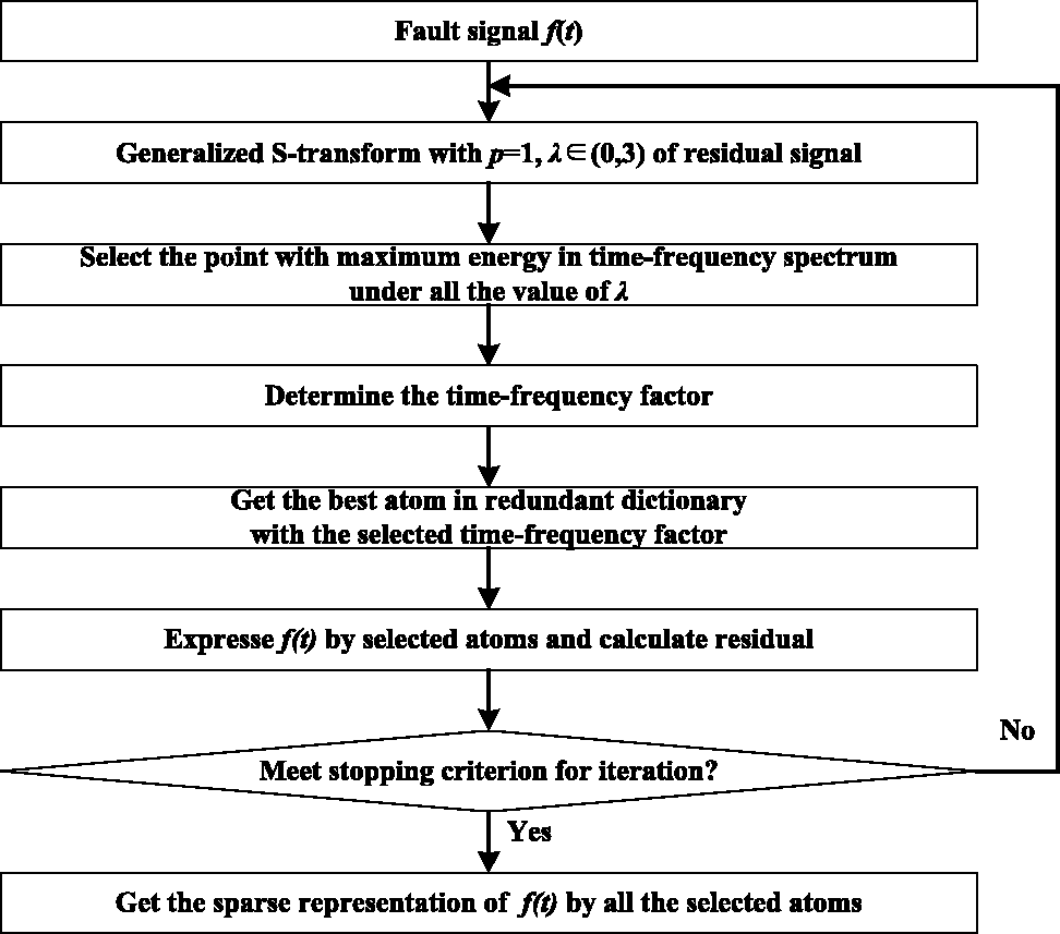
The algorithm flowchart of SD–MGST.
Whether the atom selected through MGST is the same as the atom selected through traditional OMP is the critical factor to measure the effect of SD–MGST.
The atom selected through proposed SD–MGST method would be proved to be the best matching atom.
Setting the detection signal to

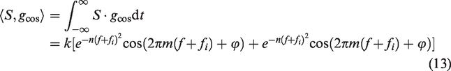
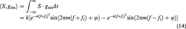
The cosine component and sine component of atom in SD–MGST is


I. Selection of optimal frequency factor f
The inner product of detection signal and cosine component is
The inner product of detection signal and sine component is
As the impulse signal has the characteristic of short duration,
It is easy to prove that when fi = f,
II. Selection of the optimal scale factor λ
After the determination of f, the inner product of detection signal and atom are
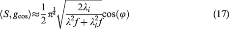
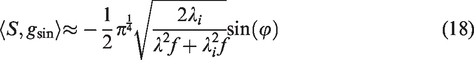
Obviously, if and only if λi = λ, they gain the maximum.
III. Selection of optimal shift factor u
After the determination of f and λ, the inner product of detection signal and atom are
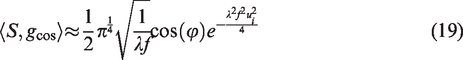
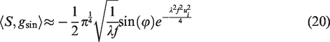
Obviously, if and only if the center coincides, they gain the maximum.
IV. Selection of optimal phase factor ϕ
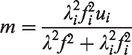
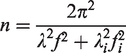
After the above three factors are extracted through the maximum energy of spectrum by MGST, ϕ can be calculated as follows
If


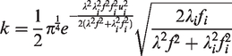
These indicate that the cosine and sine components of inner product are respectively related to the real and imaginary components of MGST. And both of them should be multiplied by
In MGST, the range of
Above all, an optimal atom in each iteration can be selected through MGST.
The decomposition steps of SD–MGST are shown as follows:
Step 1: Construct redundant dictionary
Step 2: Set residual
Step 3: Set adjustment factor of MGST
Step 4: Normalize the result of MGST,
Step 5: Update the index set in the library of selected atoms,
Step 6: Update coefficient,
Step 7: Update residual,
Step 8: Update number of iteration,
Step 9: Decide whether to stop, if stop, k = i – 1; if not, return step 3;
Step 10: Get the representation of
Simulation results and analysis
To verify the validity of the proposed SD–MGST method, three simulated signals with different SNRs would be used. Furthermore, comparison of the proposed SD–MGST method to traditional GST, OMP, and LMD are made in this section: (1) Accuracy comparison between traditional GST and proposed SD–MGST; (2) Convergence rate and accuracy comparison between traditional OMP and proposed SD–MGST; (3) Accuracy comparison between traditional LMD and proposed SD–MGST.
Simulated signals S is constructed of impulse components Sp and noise components Sn. Sp is the periodic damping signal of 3Hz, Sn is the white noise.

The intensity of Sn is changed to generate three simulated signals such as S1 with no noise, S2 with SNR = 10.36 dB, S3 with SNR = –3.62 = dB.
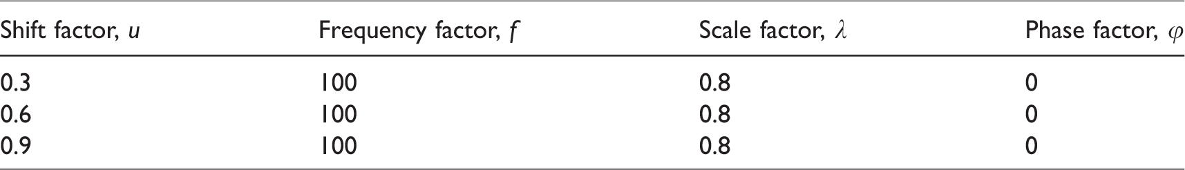
The time–frequency factors of impulses are shown in Table 1.
Time–frequency factors of impulse signal.
The waveform of three simulated signals is shown in Figure 2.
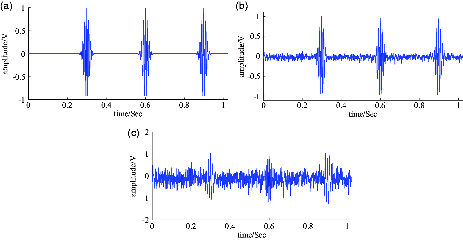
The waveform of three simulated signals: (a) signal without noise; (b) signal with noise, SNR=10.36 dB; (c) signal with noise, SNR=–3.62 dΒ.
Comparison of GST and proposed SD–MGST
Also, GST can reveal the time–frequency distribution of signals but the performance is affected by adjustment factors, which is decided by experience. To indicate the superiority of the proposed SD–MGST in impulses location, we give the comparison between GST and SD–MGST.
The adjustment factors in GST method satisfy p = 1, λ = 0.8, λ = 2, λ = 2.5; the adjustment factors in the SD–MGST method satisfy p = 1, λ ∈ (0,3). These two methods are adopted to analyze the three simulated signals respectively.
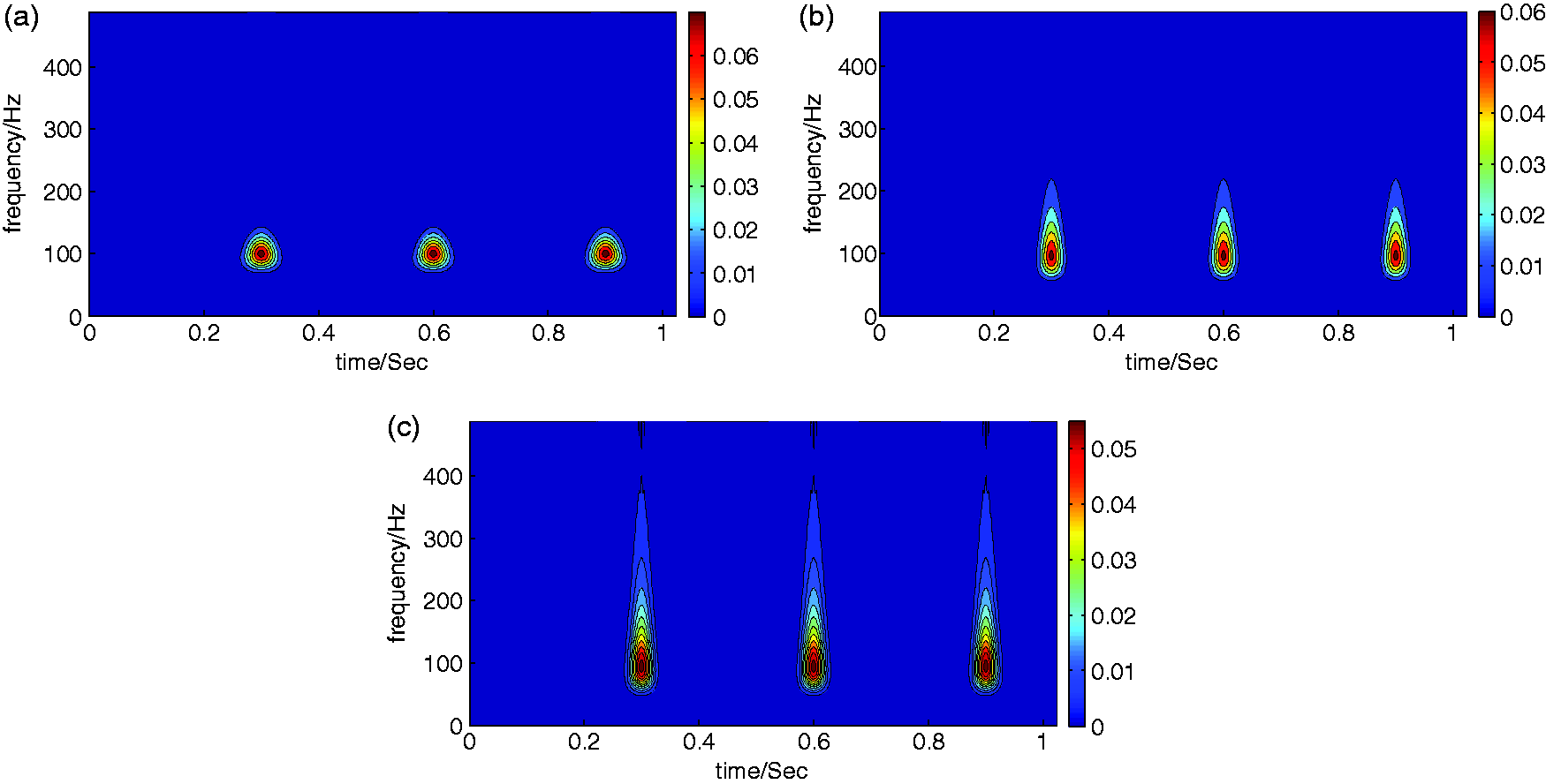
The time–frequency spectrum of S1 with GST is shown in Figure 3. The location of the local maximum energy with GST for simulated signals is shown in Table 2. The optimal time–frequency spectrum of simulated signals with the proposed SD–MGST is shown in Figure 4. The location of the local maximum energy with proposed SD–MGST for simulated signals is shown in Table 3.
The time–frequency spectrum of S1 with GST: (a)
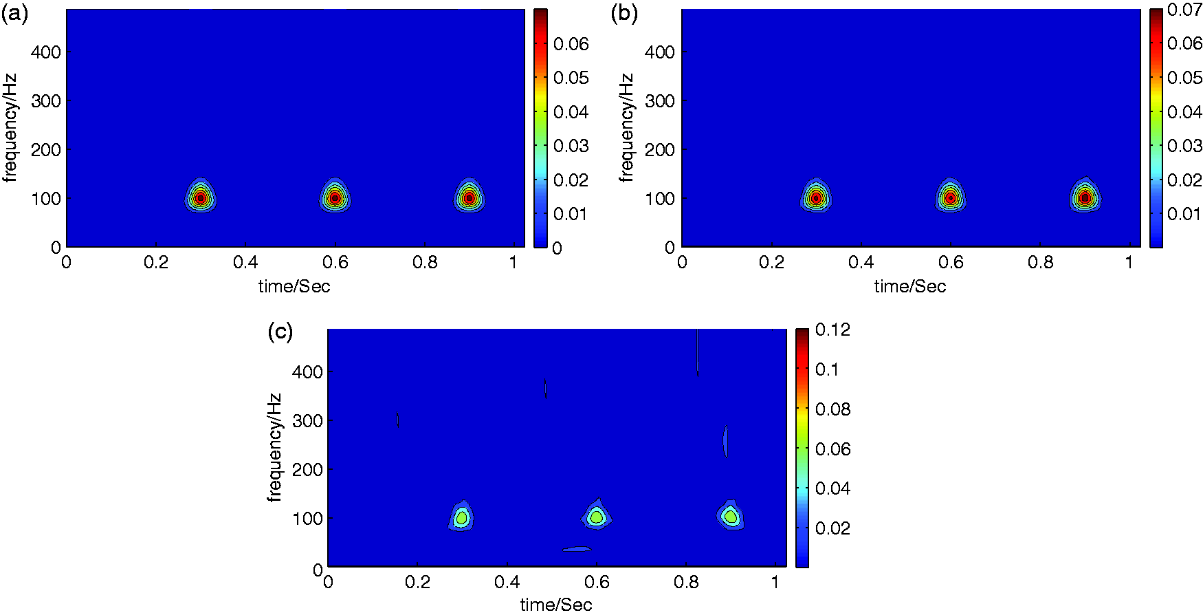
The time–frequency spectrum of simulated signals with proposed SD–MGST: (a) S1; (b) S2; (c) S3.
Location of the local maximum energy with GST.
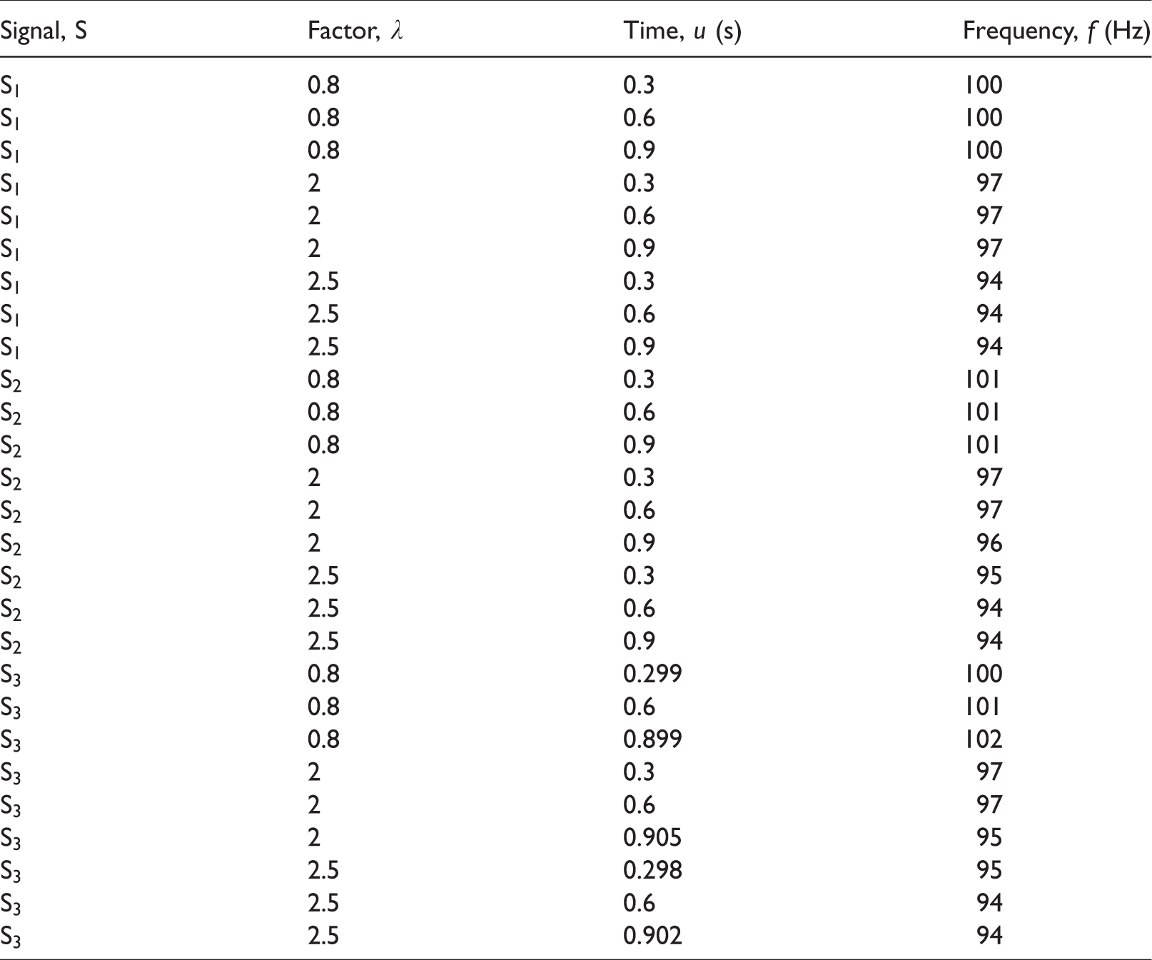
Location of the local maximum energy with proposed SD–MGST.
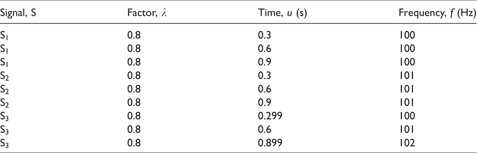
Figure 3 shows that the energies mainly focus on the time periods of 0.3 s, 0.6 s, 0.9 s and the frequency of 100 Hz. And the highest concentrations of energy is in the spectrum with λ = 0.8, in which the adjustment factor of GST and simulated signal is equal.
Table 2 shows that only when the adjustment factor of GST and impulses is equal to λ = 0.8, the location of the maximum energy with GST coincides with impulses. The location error would be occurred if the factors are unequal. Actually, it is impossible to select such a correct λ decided by experience. And the error increases with the decreasing of SNRs.
From Figure 3 and Table 2, it is obvious that the location of impulses in the time domain can be extracted effectively through GST method, but the location in the frequency domain is difficult to be extracted accurately. It is mainly because the adjustment factor is selected based on the experience in the GST method, but the time–frequency factors of impulses is unknown in the detection signal.
Figure 4 displays that the energies are highly concentrated in the time periods of 0.3 s, 0.6 s, 0.9 s and the frequency of 100 Hz with the proposed SD–MGST. And the maximum energy will decrease with the increasing of noise.
Table 3 shows that the adjustment factors are matching perfectly with the impulses with the proposed SD–MGST, and the time–frequency factors are all the same as the impulses, and are still matching effectively with minor error with the increasing of noise. Compared to Table 2, the time–frequency factors of the maximum energy are more closer to the impulses and the adjustment factor λ can be accurately extracted through SD–MGST rather than being decided by experience through GST.
Above all, the proposed SD–MGST method has better performance in the extraction of the time–frequency information.
Comparison of OMP and proposed SD–MGST
OMP can represent the impulses sparsely and accurately, but the shortcomings are the huge computation and long running time, so in this section, the running time is the main indicator between OMP and SD–MGST.
The sparse decomposition for three simulated signals with the traditional OMP method and proposed SD–MGST method is operated under the same environment. And the comparison shows the accuracy of selected atoms, running time, and approximation errors of the sparse representation.
The sparse representation for S3 with SD–MGST and OMP is shown in Figure 5. The correlation coefficient of selected atoms and S1 is shown in Table 4, the correlation coefficient of selected atoms and S2 is shown in Table 5, and the correlation coefficient of selected atoms and S3 is shown in Table 6.
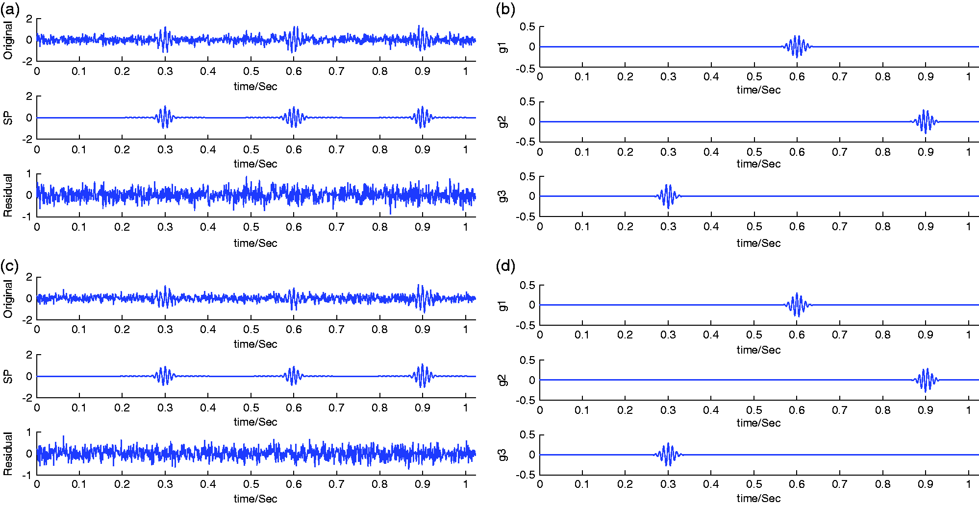
Sparse representation for S3 with SD–MGST and OMP: (a) sparse representation with SD–MGST method; (b) selected atoms with SD–MGST method; (c) sparse representation with OMP method; (d) selected atoms with OMP method
Correlation coefficient of the selected atoms and S1.
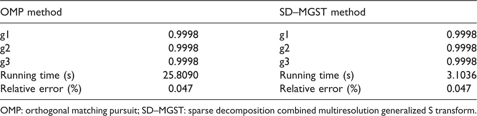
OMP: orthogonal matching pursuit; SD–MGST: sparse decomposition combined multiresolution generalized S transform.
Correlation coefficient of the selected atoms and S2.
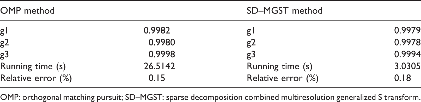
OMP: orthogonal matching pursuit; SD–MGST: sparse decomposition combined multiresolution generalized S transform.
Correlation coefficient of the selected atoms and S3.
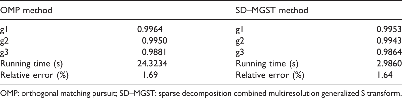
OMP: orthogonal matching pursuit; SD–MGST: sparse decomposition combined multiresolution generalized S transform.
Figure 5 shows that the weak impulses can be extracted effectively from strong noise through both traditional OMP method and proposed SD–MGST method. Tables 4 to 6 further indicate that the selected atoms through these two methods correspond closely to impulses and the approximate errors are both very small. Although the accuracy of OMP method is a little higher than the proposed SD–MGST method, the running time is much longer than SD–MGST.
So the proposed SD–MGST method has the characteristic of high accuracy and high efficiency. It can be widely used for real-time analysis.
Comparison of ELMD and SD–MGST
The decomposition for three simulated signals with traditional LMD method and proposed SD–MGST method is operated under the same environment. And the comparison is mainly in running time and approximation error.
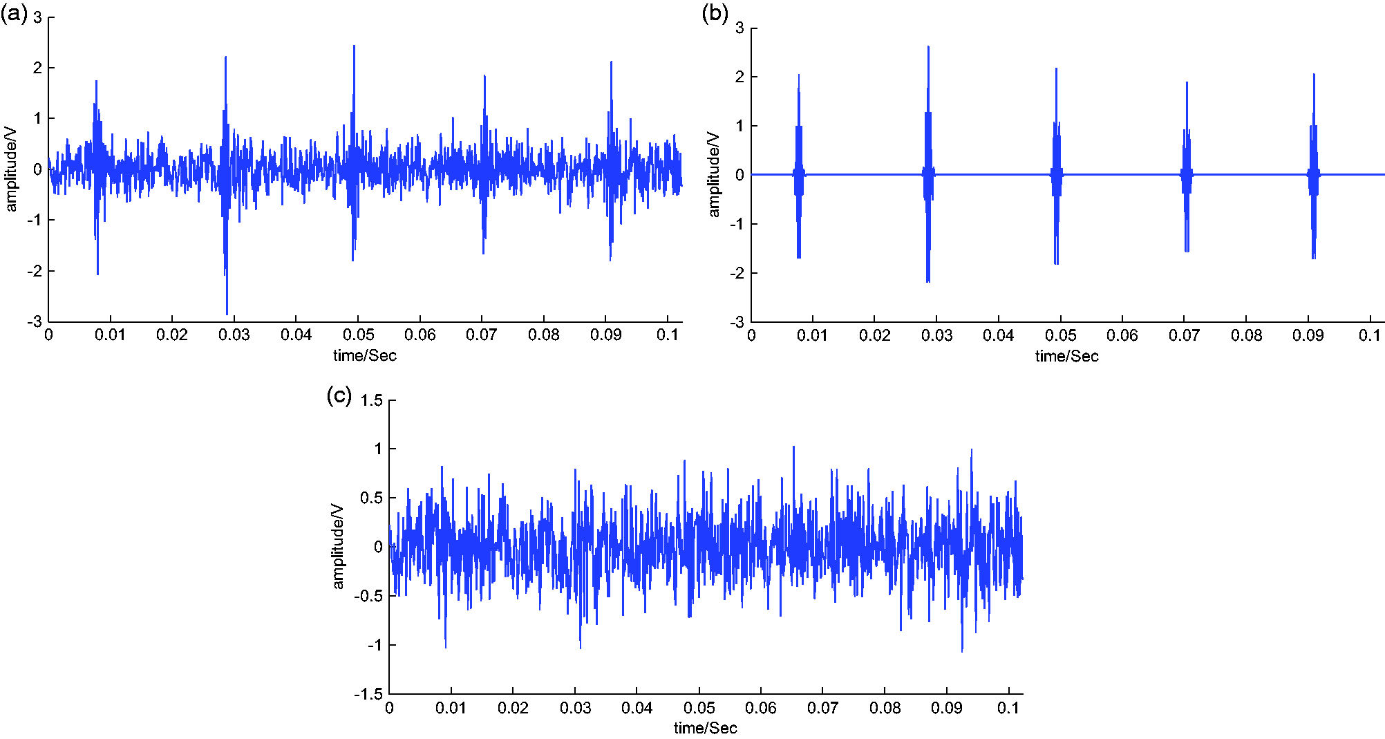
The decomposition of S3 with LMD is shown in Figure 6. The comparison for S1, S2, and S3 are shown in Table 7.
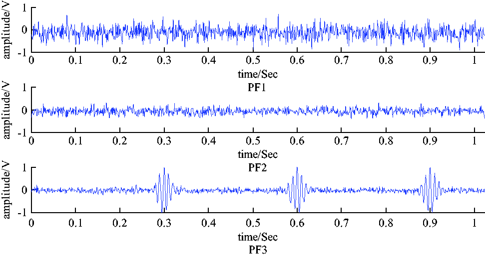
Decomposition of S3 with LMD.
Comparison of LMD and SD-TFSS for S1, S2, and S3.
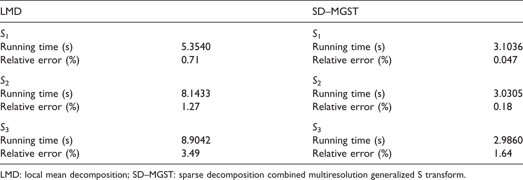
LMD: local mean decomposition; SD–MGST: sparse decomposition combined multiresolution generalized S transform.
Figure 6 indicates that the weak impulses can be decomposed effectively through LMD, but still has some noise. Table 7 indicates that the running time of the LMD method is much longer than that of the SD–MGST method, and the accuracy is also lower.
Above all, the proposed SD–MGST method can be widely used for real-time analysis with high accuracy and efficiency.
Engineering application
To verify the validity of the proposed SD–MGST method in application, two sets of outer ring fault signals are acquired from a fault test platform of rotating machinery. As the fault intensity is proportional to the rotation speed, we choose the vibration signals at 600 r/min to represent the high SNR and the signals at 150 r/min to represent the low SNR. In this platform, the rolling number of bearing is 12, rolling diameter is 7.5 mm, pitch diameter is 39.5 mm, contact angle is 0, the direction of the crack on the outer ring of bearing is along the axial direction, the width of the crack is 0.5 mm, and the depth of the crack is 0.3 mm. According to the bearing parameters, the theoretical value of fault characteristic frequency is 48.6 Hz at 600 r/min and 12.2 Hz at 150 r/min, respectively. The proposed SD–MGST method and LMD is used to extract the sparse feature.
The outer ring fault at 600 r/min with SD–MGST is shown in Figure 7, the outer ring fault at 600 r/min with LMD is shown in Figure 8, the outer ring fault at 150 r/min with SD–MGST is shown in Figure 9, and the outer ring fault at 150 r/min with LMD is shown in Figure 10.
Outer ring fault at 600 r/min with SD–MGST: (a) original fault signal; (b) sparse representation with SD–MGST method; (c) residual signal.
Outer-ring fault at 600 r/min with LMD.
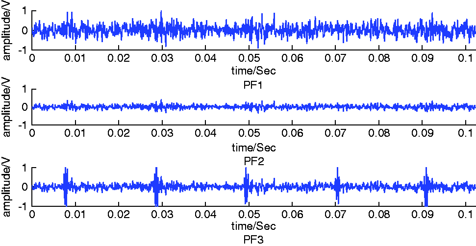
Outer ring fault at 150 r/min with SD–MGST: (a) original fault signal; (b) sparse representation with SD–MGST method; (c) residual signal.
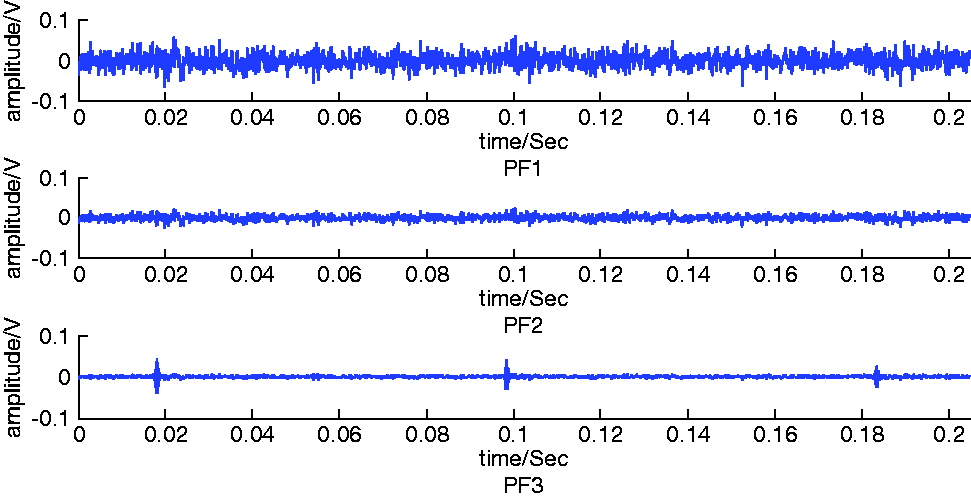
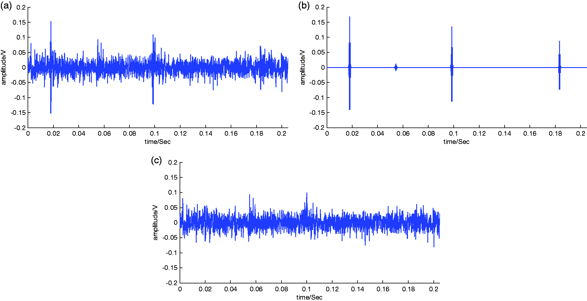
Outer ring fault at 150 r/min with LMD.
Figure 7(a) shows that the periodic impulses are mixed in underground noise, Figure 7(b) shows that the impulses are accurately extracted to represent the fault signal sparsely and the noise is filtered. Figure 7(c) shows no obvious impulses in residual. According to the sparse representation, the fault characteristic frequency is 48.1 Hz, which is consistent with the theoretical value of 48.6 Hz. Figure 8 shows the extracted impulses still have some noise, which has worse performance than that shown in Figure 7.
Figure 9(a) shows that the periodic impulses are mixed with the underground noise and the impulses are covered by strong noise. Figure 9(b) shows that the impulses are extracted to represent the fault signal sparsely and the noise is not filtered completely. Figure 9(c) shows no obvious impulses in residual. According to the sparse representation, the fault characteristic frequency is 12.1 Hz, which is consistent with the theoretical value of 12.2 Hz. Figure 10 shows that the extracted impulses still have strong noise, which has worse performance than that shown in Figure 9.
Conclusions
In this paper, a method of sparse decomposition combined multiresolution GST is proposed for fault diagnosis of rotating machinery. The results from simulation and engineering application demonstrate the superiority of the proposed method. The conclusions are summarized as follows:
The over-complete dictionary of the proposed SD–MGST method is constructed based on the vibration dynamic characteristic, and it is improved to use fast algorithm easily. The proposed SD–MGST method combines the traditional OMP method and MGST method. MGST is employed for searching the optimal atom for the OMP method. Different from the traditional GST based on empirical adjustment factors, MGST can get the precise time–frequency factors from multiresolution time–frequency spectrums. As the MGST can be realized with fast algorithm based on FFT, SD–MGST method is more efficient than OMP; meanwhile, it inherits the advantage of OMP in sparse representation for fault signals with local feature.
Footnotes
Declaration of conflicting interests
The author(s) declared no potential conflicts of interest with respect to the research, authorship, and/or publication of this article.
Funding
The author(s) disclosed receipt of the following financial support for the research, authorship, and/ or publication of this article: This work was supported by Hubei Province Key Laboratory of Intelligent Information Processing and Real-time Industrial System in Wuhan University of Science and Technology(No. znxx2018QN05), the Hubei Provincial Department of Education (No. B2016006), and the National Natural Science Foundation of China (No. 61174106).