
Abstract
The dynamic characteristics of rod fastening rotor supported by a finite journal bearing are investigated in this study. To model the dynamic behaviors of the bearing-rotor system, the oil film force of bearing is calculated by approximately solving the Reynolds equation with the variables separation method and Sturm–Liouville theory, and then a motion equation is developed with consideration of the contact and gyro effects of the disks of the rotor. To solve the motion equation with small error and excellent stability, an improved Newmark method is proposed. On this basis, the dynamics characteristics of the rod fastening rotor are analyzed for different rotor speeds, disk eccentricities, shaft bearing stiffness, and contact stiffness. And the orbits of the rod fastening rotor and integral rotor are compared. The numerical results indicate that the analytical solution of the oil film force has higher computational efficiency than the finite difference method. The rod fastening rotor shows higher stability than the integral rotor, and exhibits rich dynamic behaviors, such as periodic, qusi-periodic, period-2, period-4, and period-6.
Introduction
Rotor-bearing system is an important component in the power equipment, and its stability affects greatly the safety and normal service performance of the equipment. However, the oil film force of the bearing is usually nonlinear, and consequently causes complex and unstable dynamic behaviors of the rotor when the rotor is working under the conditions of high speed and overload. Therefore, the dynamic stability of the rotor-bearing system caused by the nonlinear oil film force has investigated by many researchers.1–6
Yang et al. 1 established the model of rotor with transverse crack by considering parametric uncertainties. And the equation of the system was solved by the Harmonic Balance method. Then, the influences of transverse crack and uncertain parameters on the responses of the rotor were studied. Wang et al. 2 studied the stability of a flexible liquid-filled rotor based on Fourier series. The analytical expression of the dynamic pressure of the liquid was derived, and the dynamic stability of the rotor was analyzed by the numerical method. Desavale et al. 3 established a comprehensive empirical model with dimensionless parameters. Based on the dimensional analysis approach, the diagnosis of misalignment and bearing looseness were studied. The calculating results of the empirical model agreed well with the experimental results. Barbosa et al. 4 predicted the rotor dynamics by using the Kriging surrogate models. The models can reduce the calculation time effectively. Zhang et al. 5 proposed an adjustable elliptical journal bearing to suppress the vibration of amplitude of the rotor, and the results indicated that the bearing can effectively reduce the vibration. Santos et al. 6 studied the dynamic characteristic of a rigid-rotor system experimentally. The damping and natural frequencies were obtained, and the maximum servovalve voltage and radial injection pressure were found for the rotor system.
In the studies above, the integral rotor was taken as the object. However, besides the integral rotor, the rod fastening rotor is also very commonly used in the heavy gas turbine and so on. For the rod fastening rotor, the rod bolts are used to press all disks tightly together. Therefore, the rod fastening rotor will show some different dynamic behaviors from the integral rotor. In this context, the dynamics characteristics of the rod fastening rotor has been studied by some researchers. Hei et al. 7 established the model of rod fastening rotor supported by fixed-tilting pad journal bearing. The database method was employed to solve the oil film force of the fixed-tilting pad journal bearing. The dynamics behaviors of the rotor system were investigated by the orbit diagrams, the time series, the frequency spectrum diagrams. But, the gyro effects of the disks were not taken into account when modelling. Zhang 8 studied the tangential contact stiffness of the disks of the rod fastening rotor based on the fractal contact theory. The correctness of the fractal contact theory was verified by experiment. At the same time, it was found that the fractal contact theory has its scope of application. The study only solved the tangential contact stiffness, but the dynamics behaviors of the rod fastening rotor were not analyzed. Li 9 established the model of rod fastening rotor by considering the contact friction force and pre-tightening force of the disks. The effects of the contact friction force and pre-tightening force on the rotor dynamics were studied. The results shown that the contact stiffness and the natural frequency of the system increased with the increase of pre-tightening force. Hu et al 10 derived the motion equation of the rod fastening rotor by Lagrange equation. The influence of the initial deflection caused by the unbalanced pre-tightening force on the dynamic behaviors of the rotor was studied. Their work showed that the initial deflection has a great effect on the rotor dynamics. Meanwhile, Hu et al. 11 also studied the dynamic characteristics of the rub-impact rod fastening rotor. The bifurcation diagram, vibration waveform, frequency spectrum, shaft orbit, and Poincaré map were used to analyze the dynamics responses of the rotor system. However, in the works of Hu et al. 11 , the influence of the gyro effect on the dynamic behaviors of the rod fastening rotor was not considered, and a short bearing model was assumed.
For the rod fastening rotor, the hydrodynamic sliding bearing is usually taken as the supporting part, and the oil film force of the bearing is very important for the analysis of the dynamic behaviors of the rotor. So, the investigation of the oil film force was implemented by many researches. In many studies, the model of infinite long bearing and infinite short bearing12–14 were adopted widely. Considering journal bearing parametric uncertainties, Ramos et al. 12 studied the dynamics of the rotor system, and the rotor is supported by the short fluid film bearings. Wei et al. 13 studied the nonlinear dynamic behaviors of the multi-disk rotor-bearing-seal system which supported by short bearing. The response of the system was calculated by the fourth order Runge–Kutta method. Liu et al. 14 studied the dynamics characteristics of the rod fastening rotor which supported by the infinite long bearing. The shooting method and path-following technique were adopted to calculate the dynamics responses of the system.
The infinite long bearing and infinite short bearing models are very simple and idealized models. In practice, the slide bearings are finite long bearings. So, the two idealized models cannot describe the actual bearing. In order to solve the oil film force of finite long bearing accurately, numerical methods are proposed. Smolík et al. 15 studied the shape of the threshold curve for a rigid rotor supported by journal slide bearing. In order to solve the oil film force of journal bearing, the four methods were proposed: the infinitely short approximation, the infinitely short approximation, the finite differences method, and the finite elements method. Tuckmantel 16 investigated the vibration signature of rotor-coupling-bearing system by solving the oil film force of the bearing with finite volume method. Lu et al. 17 calculated the oil film forces and their Jacobis by the variational constraint approach. However, the numerical methods (such as the finite volume method, finite elements method, finite differences method, and variational constraint approach) have large calculation cost.
In this study, an approximation analytical solution of oil film force is proposed for the supporting bearing of the rod fastening rotor by using the method of separation of variables and Sturm–Liouville theory. This method not only ensures the calculation accuracy, but also improves the calculation efficiency. Meanwhile, a model of the rod fastening rotor is established by considering the Gyro effect and contact effect of the disks, and an improved Newmark method is proposed to solve the dynamic responses of the rotor system. On this basis, the comparison of obit is implemented between the integral rotor and rod fastening rotor. The influence of rotating speed, eccentricity, bending stiffness, and contact stiffness on the dynamic behaviors of the rotor system is also investigated.
Equation of the rod fastening rotor system
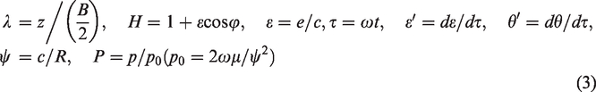
The geometry model of the rod fastening rotor system supported by oil film hydrodynamic journal bearings is given in Figure 1. In this study, the contact effect and gyro effect of the disks are considered, and the contact effect of disks is taken as a bending spring with nonlinear stiffness. 18
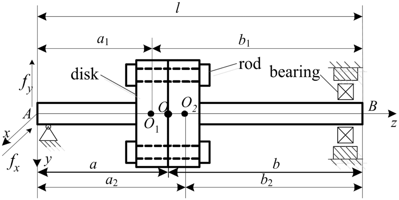
Schematic diagram of the bearing-rod fastening rotor system.
In Figure 1, O1 and O2 are the centers of the two disks, l is the length of the whole rotor, a and b are the length of the two shafts, a1 is the distance between A and O1, b1 is the distance between B and O1, a2 is the distance between A and O2, b2 is the distance between B and O2, mO1 and mO2 are the mass of disk O1 and O2, mA and mB are the mass of the two shafts (the length are a and b respectively), eO1 and eO2 are the eccentricities of the disk O1 and O2, fx and fy are the nonlinear oil film forces of bearing in negative x and y directions, respectively.
Coordinate of finite length journal bearing.
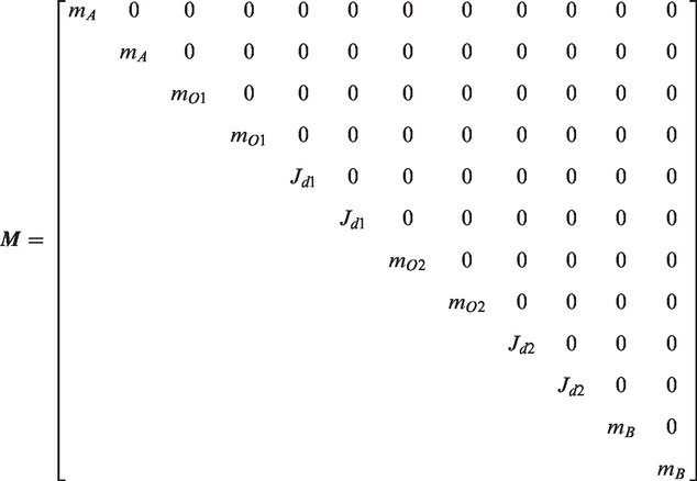
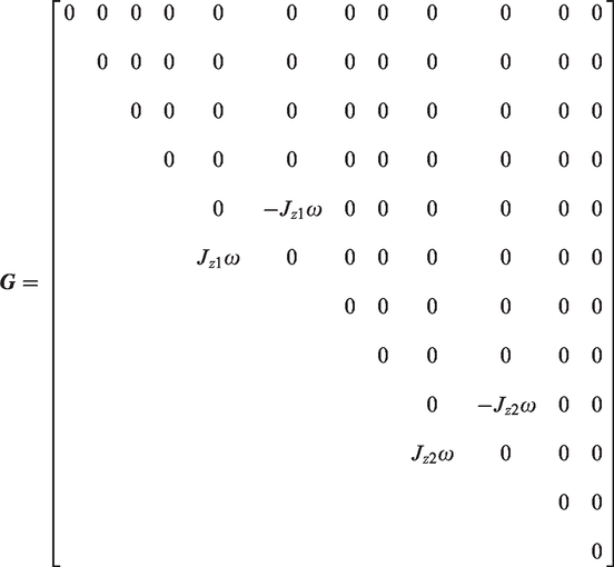
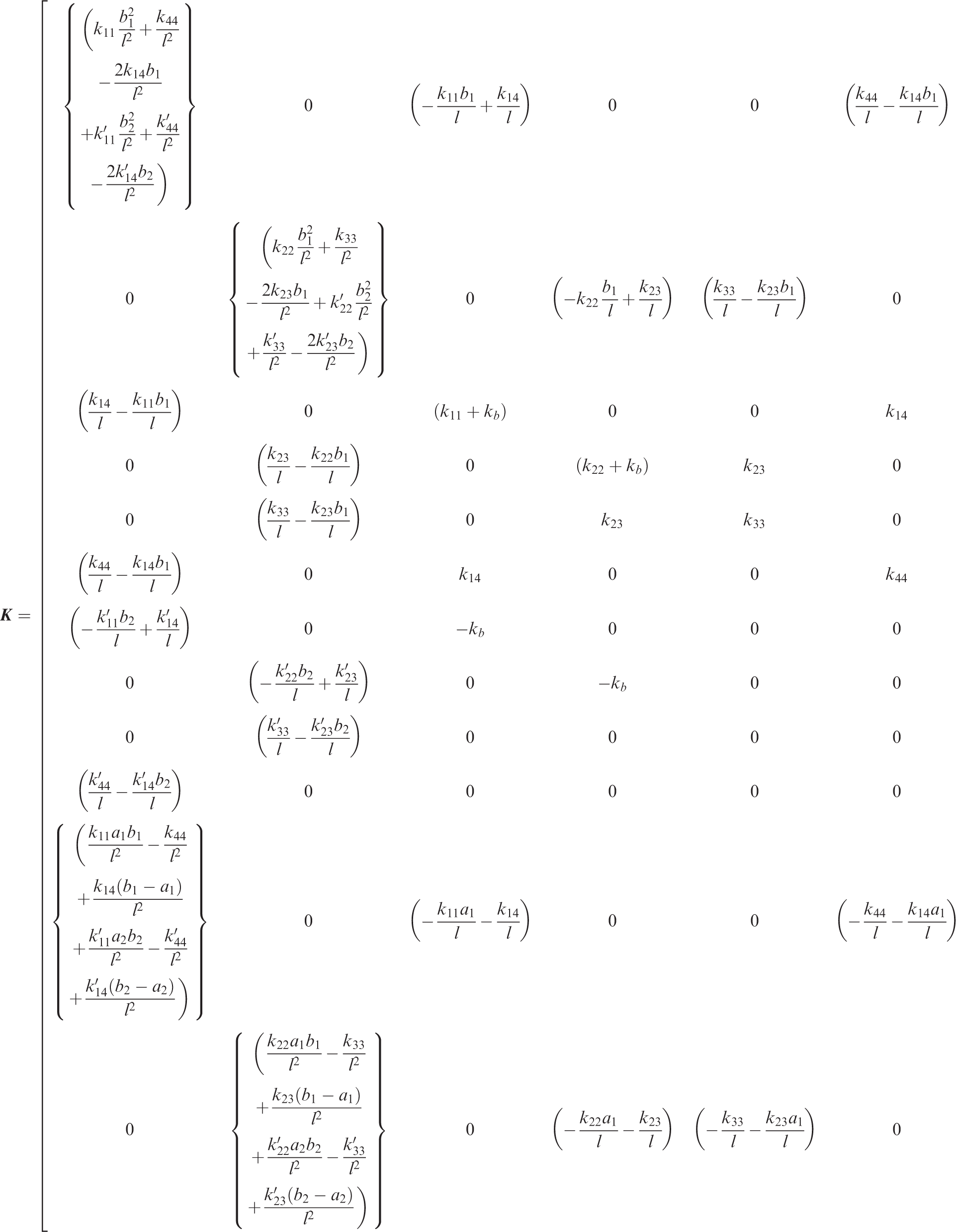
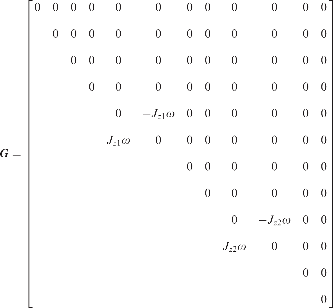
The dynamic equation of the rod fastening rotor system can be written as follows

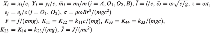
For the convenience of calculating and derivation, the following dimensionless variables are introduced.
Nonlinear oil film force
Solution of nonlinear oil film force
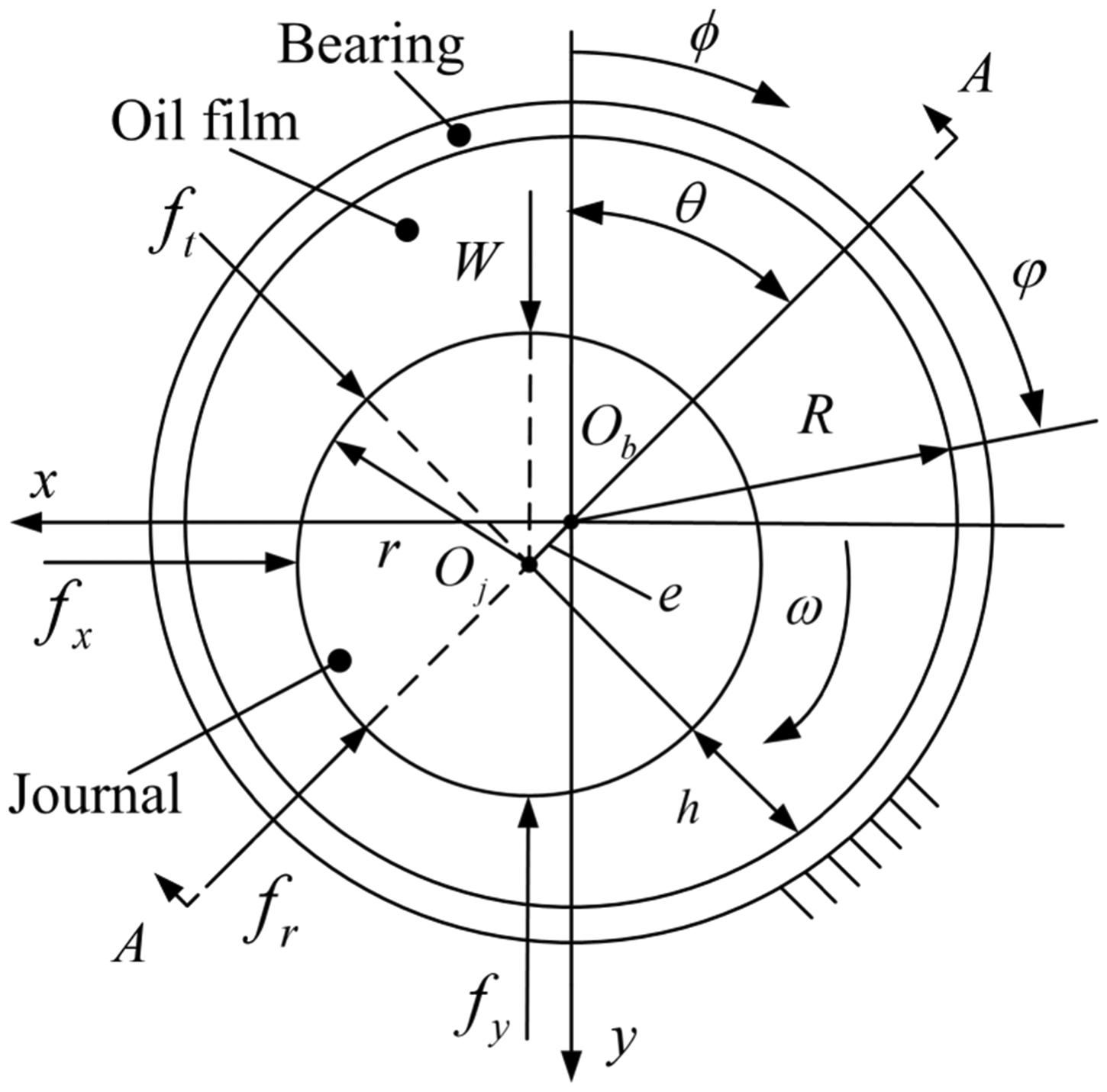
The geometry of the journal bearing is shown in Figure 2, and the cross section of the bearing is shown in Figure 3. In the two figures, Ob is the center of the bearing, Oj is the center of the shaft journal, θ is the deviation angle, Φ is the angle goes from negative y-axis direction along the clockwise direction, φ is the angle which goes from extension of OjOb along the clockwise direction, fr and ft are oil film forces in the negative radial and the tangential directions, fx and fy are oil film forces in negative x and y directions, h is the thickness of oil film, R is the radius of the bearing, and W is the load of the bearing.
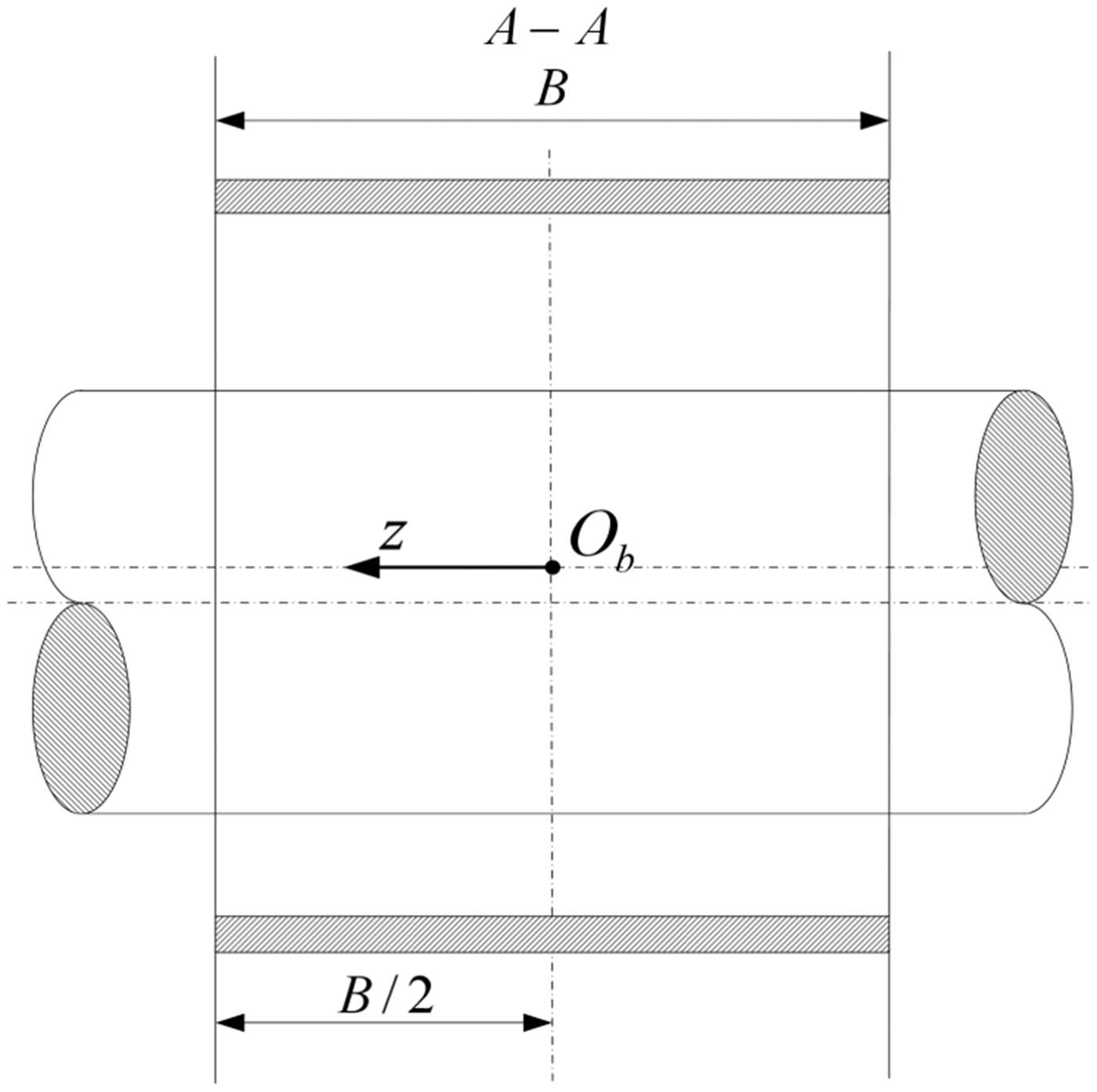
The cross section of the finite length journal bearing.
By assuming that the lubricant is in-compressible, the Reynolds equation for the lubrication of the journal bearing can be written as
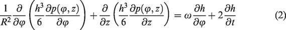
For the convenience of derivation and calculation, the dimensionless variables are introduced as follows
Substituting the dimensionless variables into equation (2), the dimensionless Reynolds equation can be written as

To solve equation (4), the method of separation of variables and Sturm–Liouville theory are used. Based on the method of separation of variables, the dimensionless oil film pressure P can written as


In equation (5), it can be seen that Pp(φ, λ) and Ph(φ, λ) determine the oil film pressure distribution P. Therefore, Pp(φ, λ) and Ph(φ, λ) need to be solved respectively, and their solutions are introduced in the next section.
Calculation of special solution
Substituting equation (6) into equation (4), the dimensionless Reynolds equation can be written as

The expression for the left item of equation (8) is a function of λ, and the expression for the right item of equation (8) is a function of φ.
Let

Pp2(λ) can be obtained by integrating equation (9) twice.

In equation (11), C is arbitrary constant, c1 and c2 are integral constants. Let C = 0, c1 and c2 can be obtained by solving the boundary conditions. The boundary conditions of the special solution in the axial direction are as follows

Based on equation (12), the constant c1 and c2 are obtained, and c1 = c2 = 0.
Let
Substituting equation (13) into equation (10),


In order to obtain the expression of Pp1(φ), Sommerfeld transformation is introduced as follows
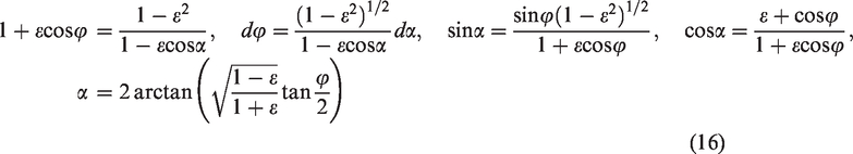
Based on Sommerfeld transformation, expression of Pp1(φ) can be written as follows
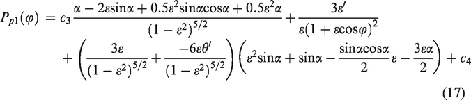
The boundary conditions of the special solution in the circumferential direction are as follows

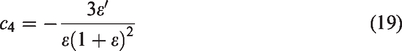
Based on the boundary conditions (i.e., equation (18)), c3 and c4 can be expressed as follows
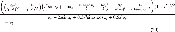
The special solutions of the oil film force in the radial and tangential directions can be obtained by integrating the Pp(φ, λ), and they can be written as follows
Calculation of general solution
By substituting Ph(φ, λ) into equation (4), then the equation (4) can be written as follows

Substituting equation (7) into equation (22), the following expression can be obtained

In order to solve the equation (23), the following expressions should be satisfied
For the journal bearing, the following boundary conditions should be satisfied

Based on the boundary conditions above, the axial boundary conditions for the general solution is obtained
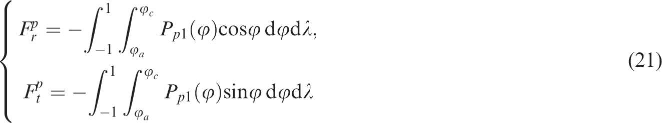
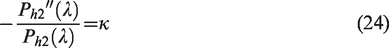
In order to solve equation (24), three situations of κ need to be considered (i.e., κ > 0, κ = 0, and κ < 0). when κ = 0
Equation (24) can be written as

By integrating the equation (28) twice, the expression of Ph2(λ) can be obtained as follows 2. when κ > 0

Let κ = k2, the solution of equation (24) is as follows 3. when κ < 0

Let κ = −k2, the solution of equation (24) can be expressed as follows


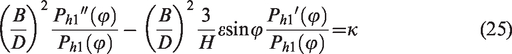
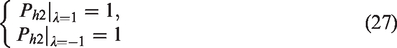
To solve the equation (25), the following transformations are adopted

Equation (25) can be expressed as Strum–Liouville equation based on equation (33), and then the equation (25) can be written as follows
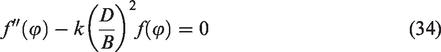
The boundary conditions of the equation (34) are as follows

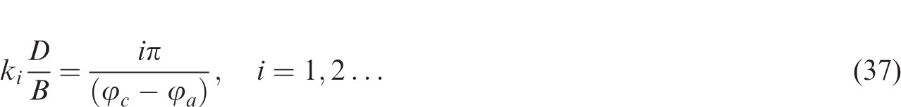
Equations (34) and (35) are taken as Strum–Liouville equation, and the equation (34) can be expressed as follows

The eigenvalue and eigenfunction of equation (36) can be obtained directly as follows

Then, general solution can be expressed as follows

The general solutions of the oil film force in the radial and tangential directions can be obtained by integrating Ph(φ, λ), and they are expressed as
Nonlinear oil film force
According to the equations (21) and (41), the nonlinear oil film forces in the radial and tangential directions can be expressed as follows

The expressions of the nonlinear oil film force in the x and y directions are as follows
Verification of the proposed method
To verify the proposed solution method of nonlinear oil film force of the bearing. The nonlinear oil film forces of bearing calculated by the proposed method, the finite difference method, 20 and the infinite long bearing model are compared. In the verification, the parameter of the bearing is listed as follows: B/d = 1, ε = 0.5, xʹ = 0.1, yʹ = 0.2, and i = 30. The comparison result is shown in Figure 4. From Figure 4, it can be seen that the oil film force calculated by the proposed method is in good agreement with the result calculated by the finite difference method. Meanwhile, the calculation time of the proposed method and the finite difference method are also compared, and shown in Figure 5. From Figure 5, it can be seen that the calculation time of the proposed method is smaller than that of the finite difference method. The results of Figures 4 and 5 indicate that the proposed method not only ensures the calculation accuracy, but also improves the calculation efficiency.
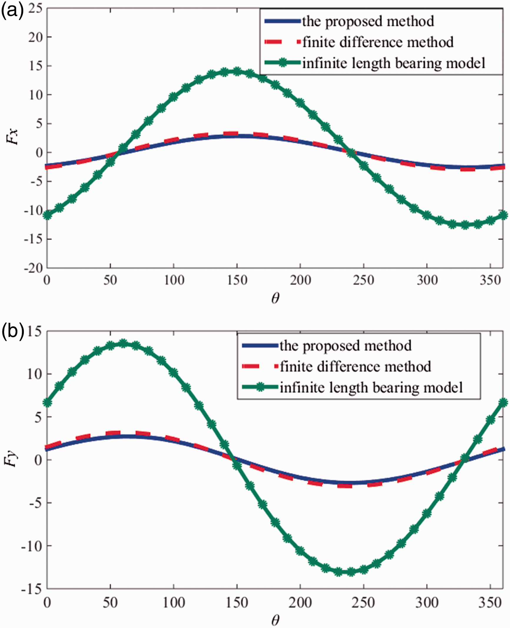
Nonlinear oil film forces versus eccentric angle θ. (a) Fx versus θ; (b) Fy versus θ.
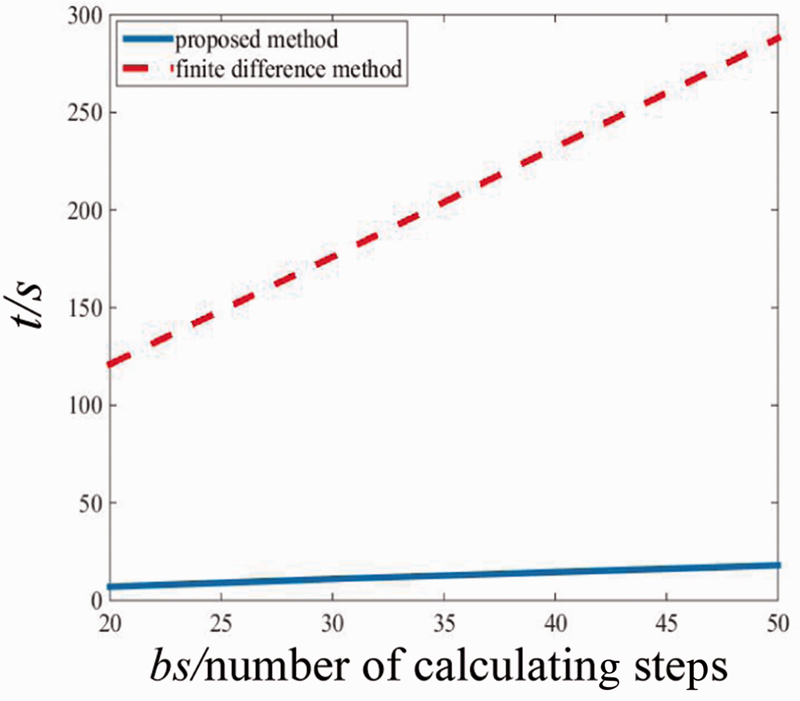
Comparison of calculation efficiency of two method.
Solving method of nonlinear dynamics
Improved Newmark method
The Newmark method is usually based on an assumption of constant acceleration. It is also called constant average acceleration hypothesis. The solution process of the Newmark method is as follows
At time t + Δt, the equation (1) can be written as follows

According to the constant average acceleration hypothesis, the following equations can be obtained


Based on constant average acceleration hypothesis,


By substituting the equations (47) and (48) into equation (44), and then the equation (44) can be written as


Substituting the values of

It should be noted that
In order to made the displacement, velocity, and acceleration satisfy the motion constrained condition and dynamic equation simultaneously, the Newmark method is improved as follows.
From the equations (47) and (50), it can be seen that Newmark method will produce an imbalance acceleration (

By substituting the equation (51) into equation (50), the following equation can be obtained

In order to eliminate the increment of dynamic load in equation (52), an increment equation of dynamics can be obtained, and it is as follows


By adding equation (52) to equation (53), and the increment of dynamic load is eliminated. And then the displacement, velocity and acceleration at the time (t + Δt) can be written as follows


From the analysis above, it can be seen that the solution of the improved Newmark method not only satisfies the motion constrained condition, but also satisfies dynamics equation basically.
Verification of the improved Newmark method
In order to verify the improved Newmark method, a model of the rotor bearing system 21 is adopted. The comparison of the calculating results among Newmark method, improved Newmark method and Runge–Kutta method is implemented.
In the verification, the parameters of the rotor-bearing system are as follows: the width of the bearing B = 0.16 m, the width to diameter ratio B/d = 1, the viscosity of lubricating oil μ = 0.02626 Pa s, the radius clearance c = 0.000288 m, the parameter of system s = 0.2662. The equivalent dimensionless mass of the rotor at the two bearing stations are
Figure 6 shows the bifurcation diagrams which calculated by the proposed method (i.e., improved Newmark method) and Newmark method. From Figure 6, it can be seen that the dynamic behaviors of the rotor can be investigated for a wide range of speeds when the improved Newmark method is adopted. Figure 7(a) shows the orbit of the rotor calculated by the improved Newmark method, Newmark method and Runge–Kutta method when
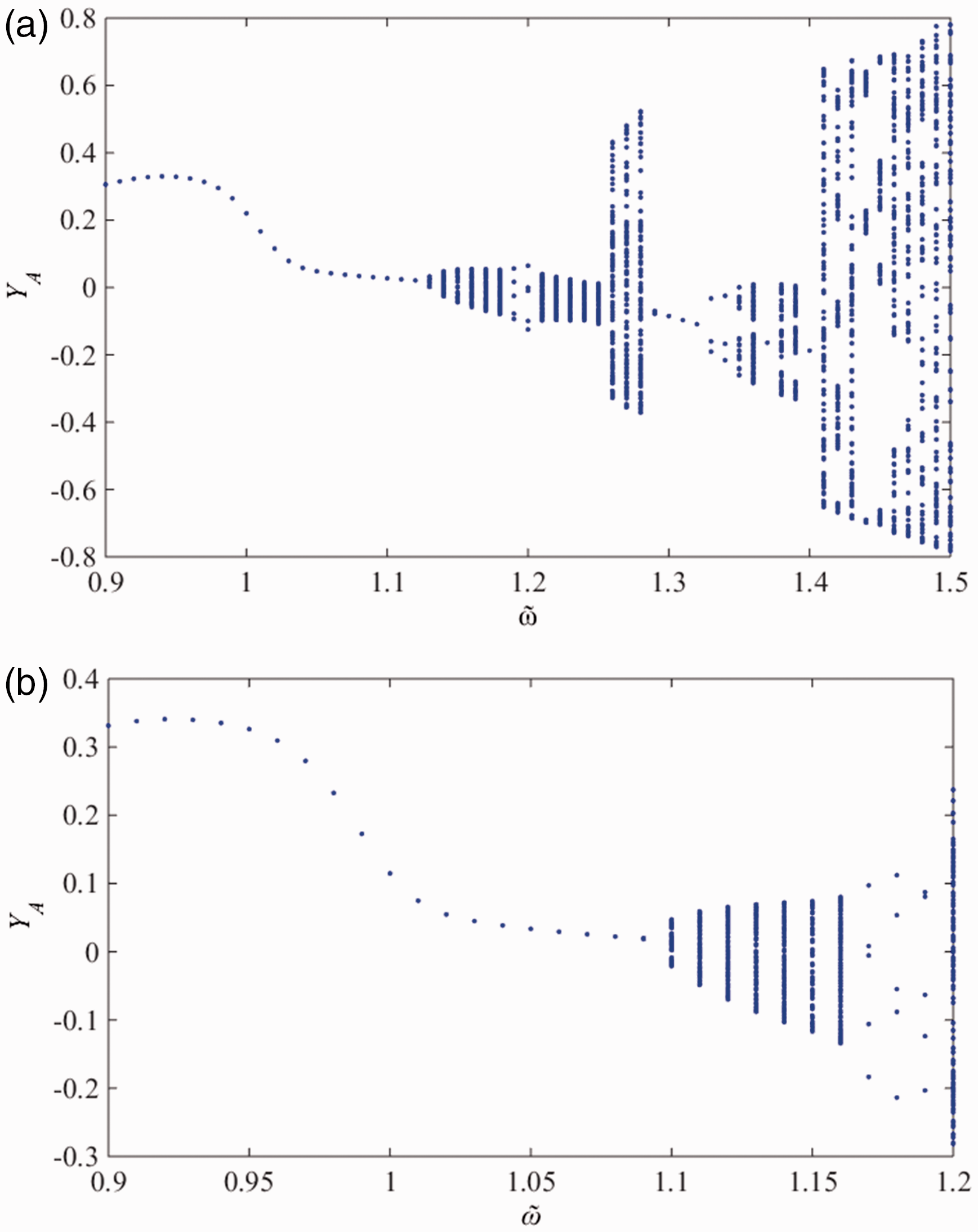
The bifurcation diagram calculated by improved Newmark method and Newmark method. (a) Bifurcation diagram calculated by the proposed method; (b) Bifurcation diagram calculated by Newmark.
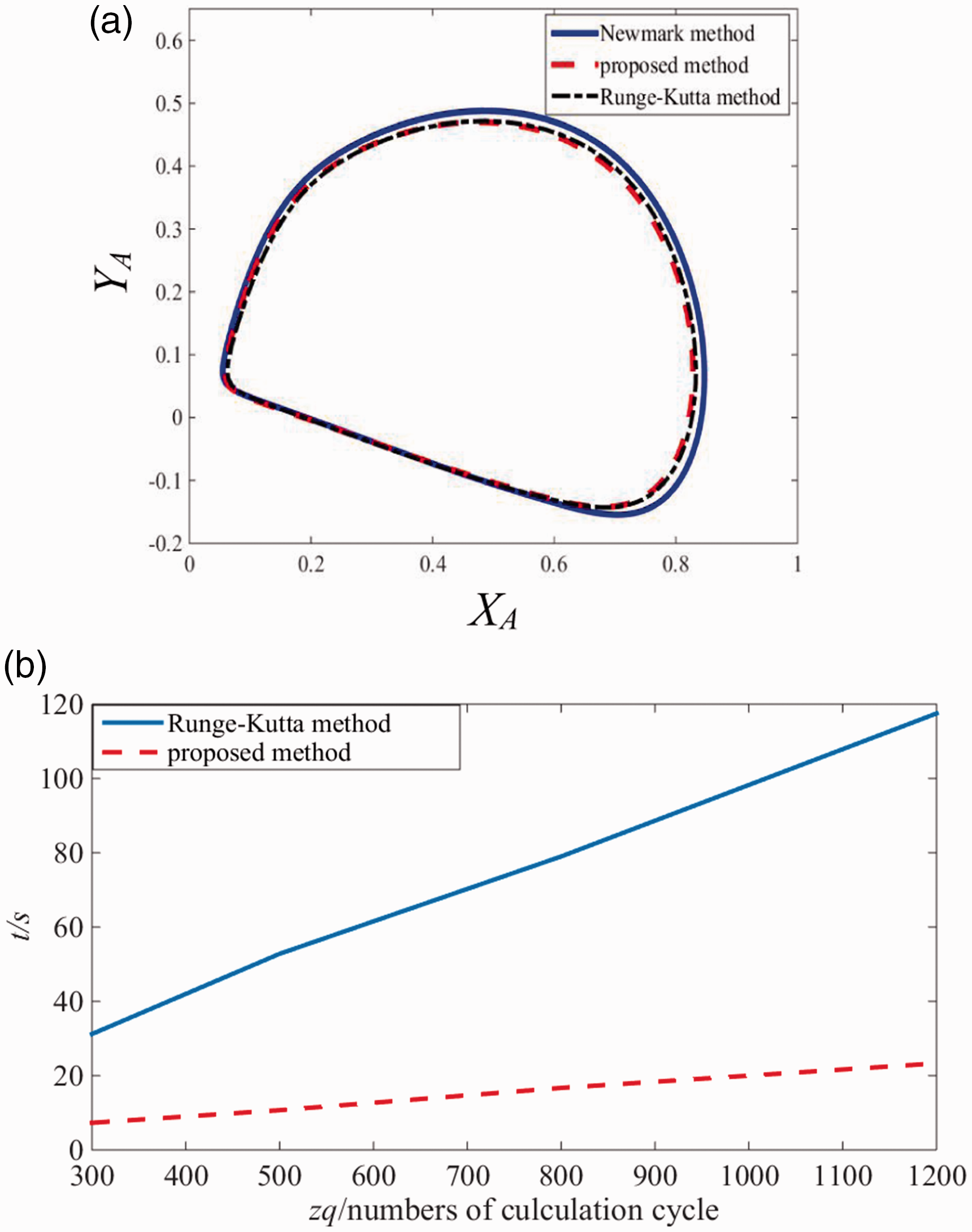
The comparison of obits and calculation efficiency between Runge–Kutta method and the improved Newmark method. (a) Obits calculated by the three method for
Numerical examples and results
The rod fastening rotor is adopted, and the oil film force is calculated by the proposed method. The improved Newmark method is adopted to calculated the dynamic response of the rod fastening rotor-bearing system. The parameter of the rotor system are as follows: r = 0.075 m, l = 3 m, a = 1.5 m, b = 1.5 m, a1 = 1.3 m, b1 = 1.7 m, a2 = 1.7 m, b2 = 1.3 m, mA = mB = 206.75 kg, h = 0.4 m (the width of disks), R = 0.16 m, eO1 = eO2 = 0.3c (i.e., ε = 0.3), mo1 = mo2 = 250.93 kg, Jz1 = Jz2 = 3.2118 kg·m2, Jd1 = Jd2 = 1.6059 kg·m2, 2 m = mA + mB + mo1 + mo2, m = 457.668 kg, B = 0.15 m, c = 0.000195 m, μ = 0.02 N·s/m2. The stiffness of the shafts are as follows: k11 = k22 = k′11 = k′22 = 1.0116 × 10⁷ N/m, k14 = k23 = −3.7733 × 10⁶ N, k′14 = k′23 = 3.7733 × 10⁶ N, k33 = k44 =k′33 = k′44 = 2.0847 × 10⁷ N·m, kb = kR = 5k11/3. The number of eigenvalue i = 30.
The comparison of the dynamic behaviors is implemented between the integral rotor and rod fastening rotor. Figure 8(a) and (b) show the orbits of the rotor at bearing station for
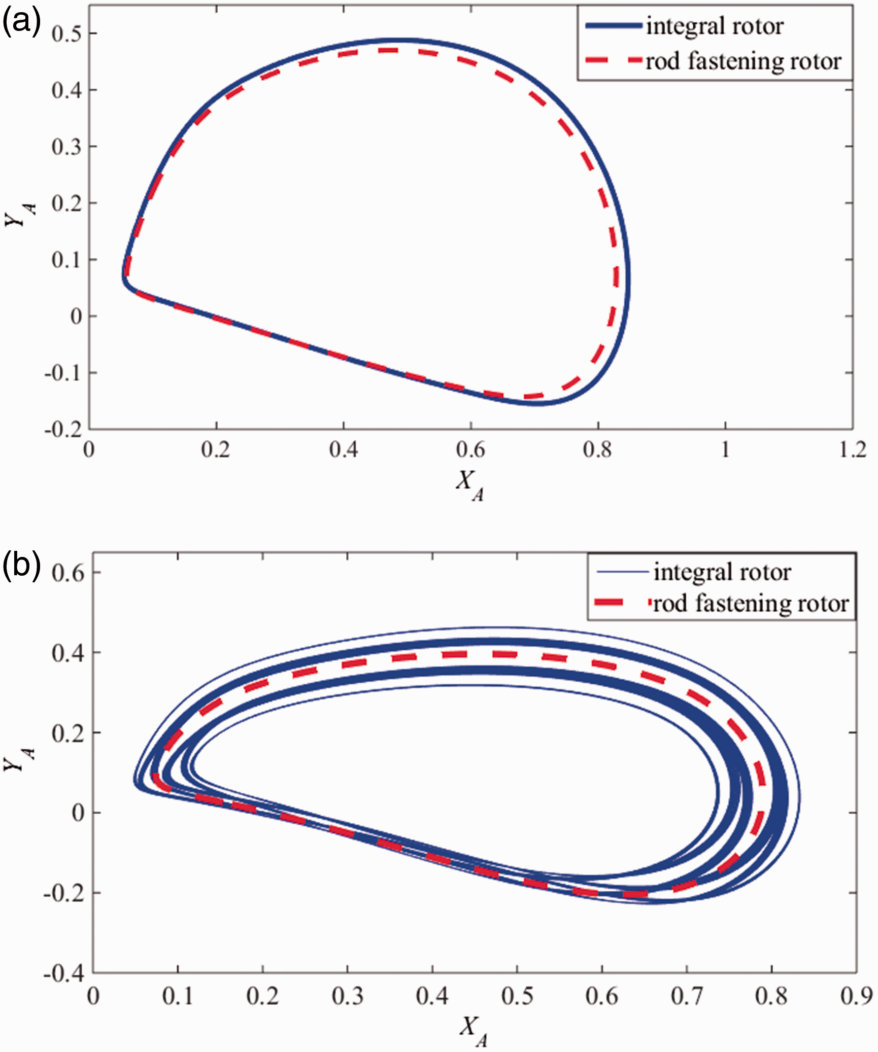
The results of the two models for
Taking the dimensionless speed as control parameter
Taking the dimensionless speed
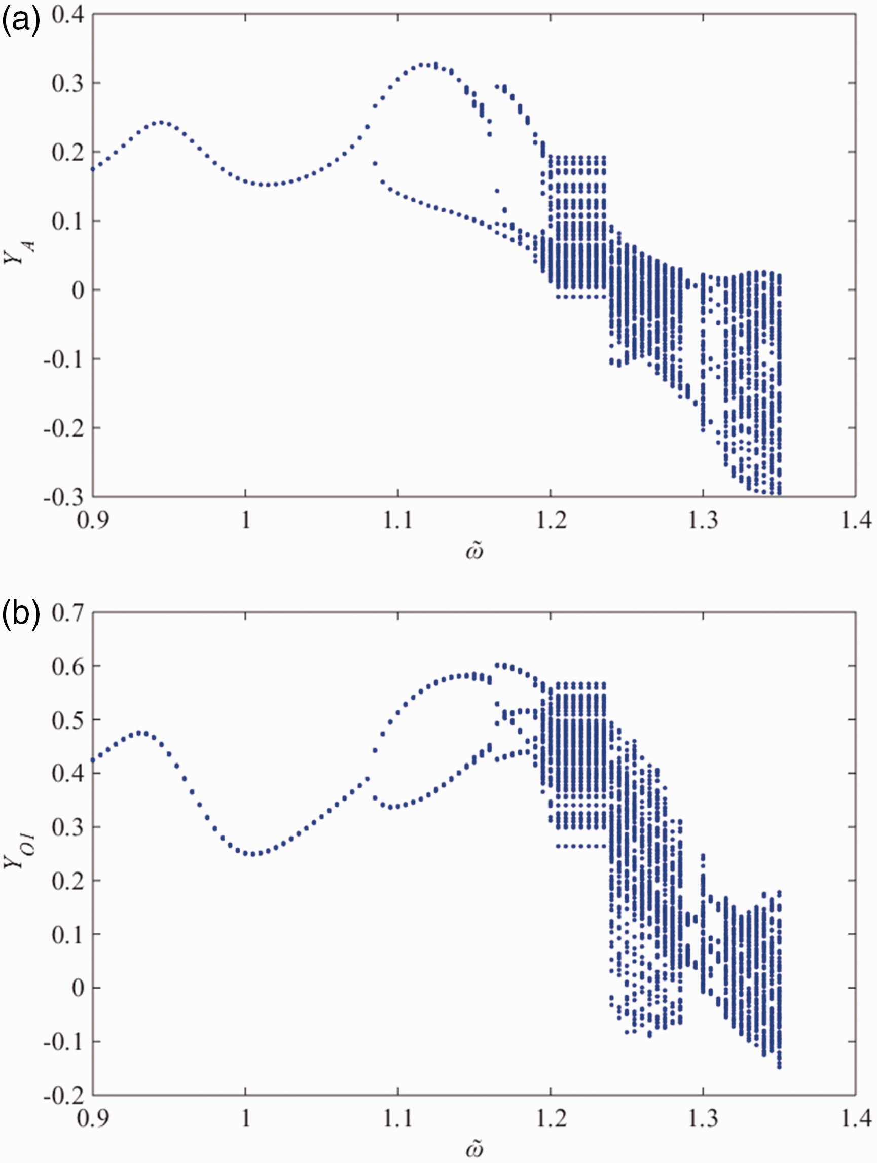
Bifurcation diagram of y versus
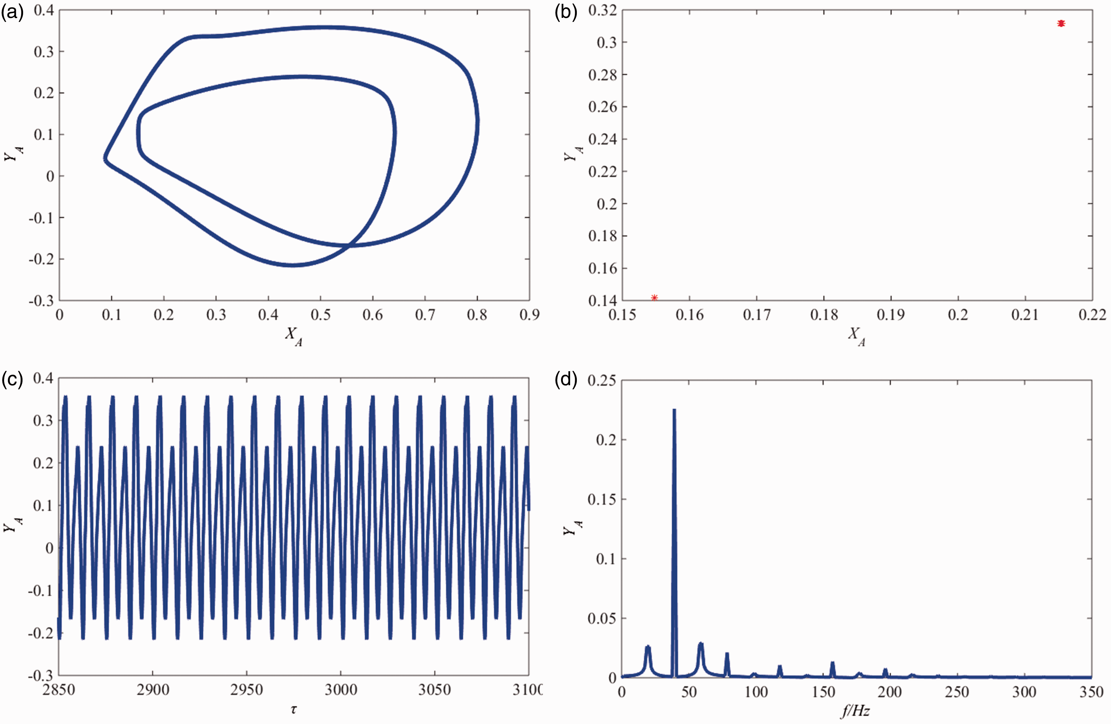
When
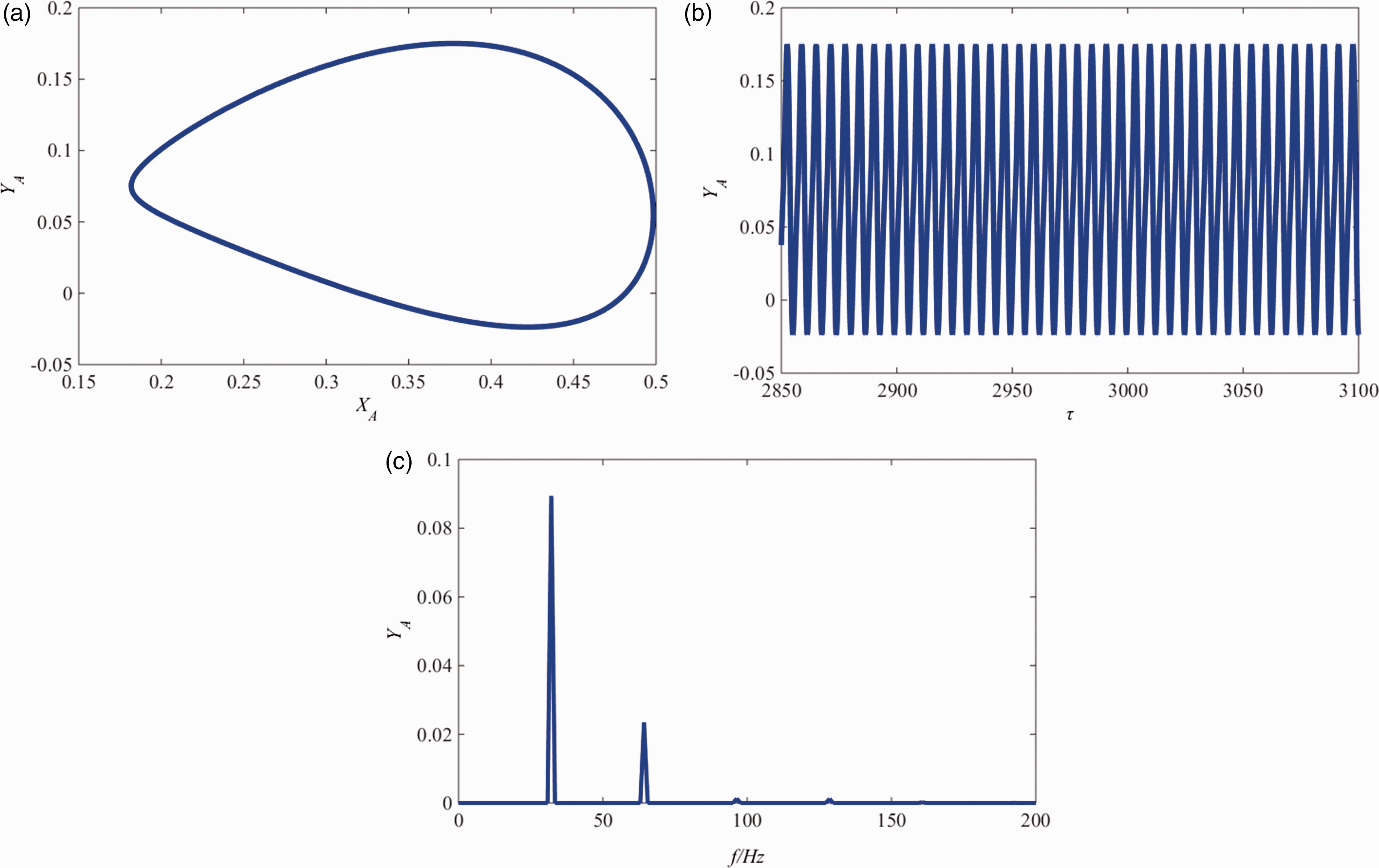
The orbit, time series and spectrum of the rotor at bearing station for
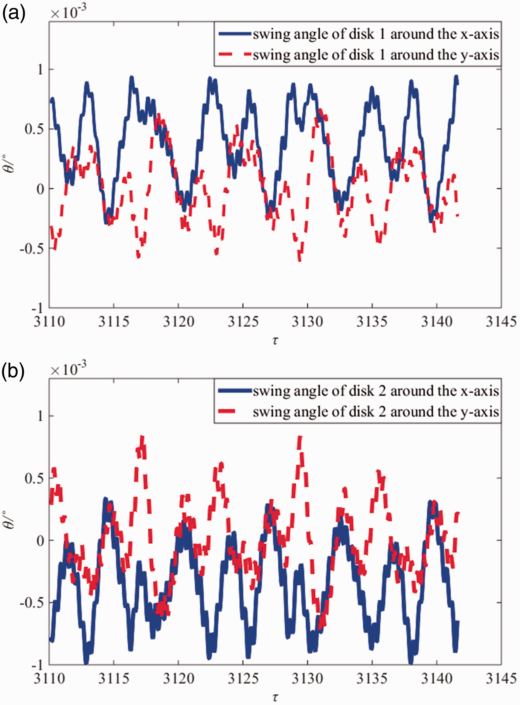
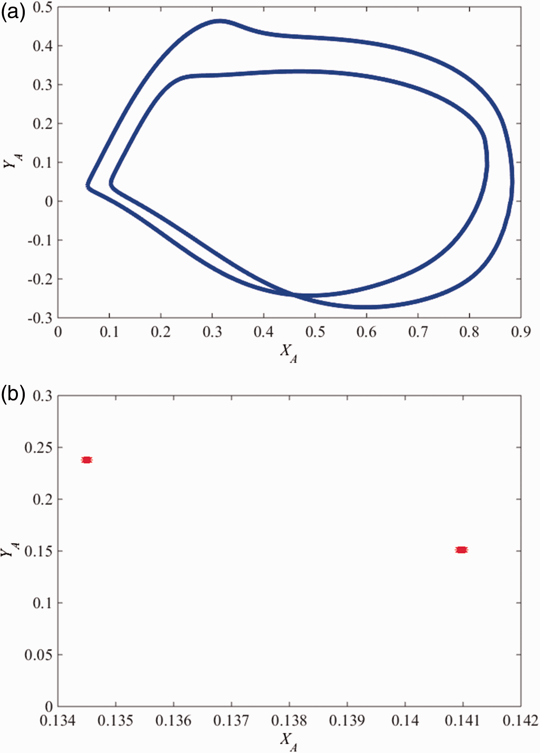
Figure 11 shows the swing angles of the two disks. In Figure 11, it can be seen that the swing angles of the disks also change periodically. With the increase of the rotating speed, the stable periodic response of the rotor system changes to period-2 response. Figure 12 shows the orbit, Poincaré map, time series and spectrum of the rotor at bearing station when
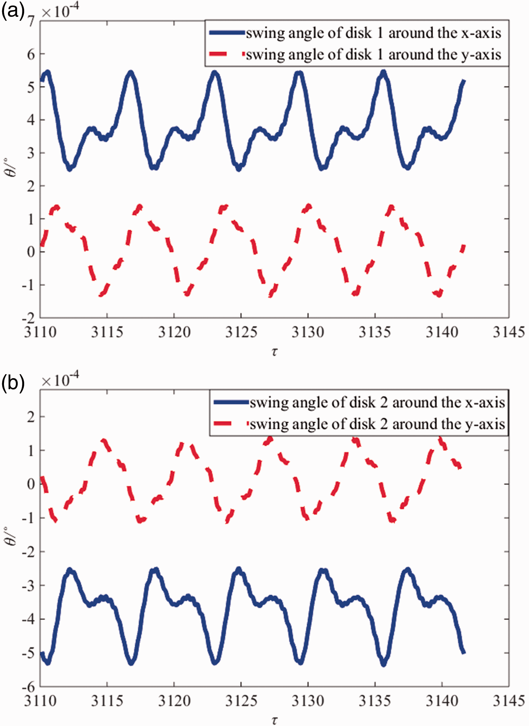
The swing angle of disks 1 and 2 around the x and y axis for
The orbit, Poincaré map, time series and spectrum of the rotor at bearing station for
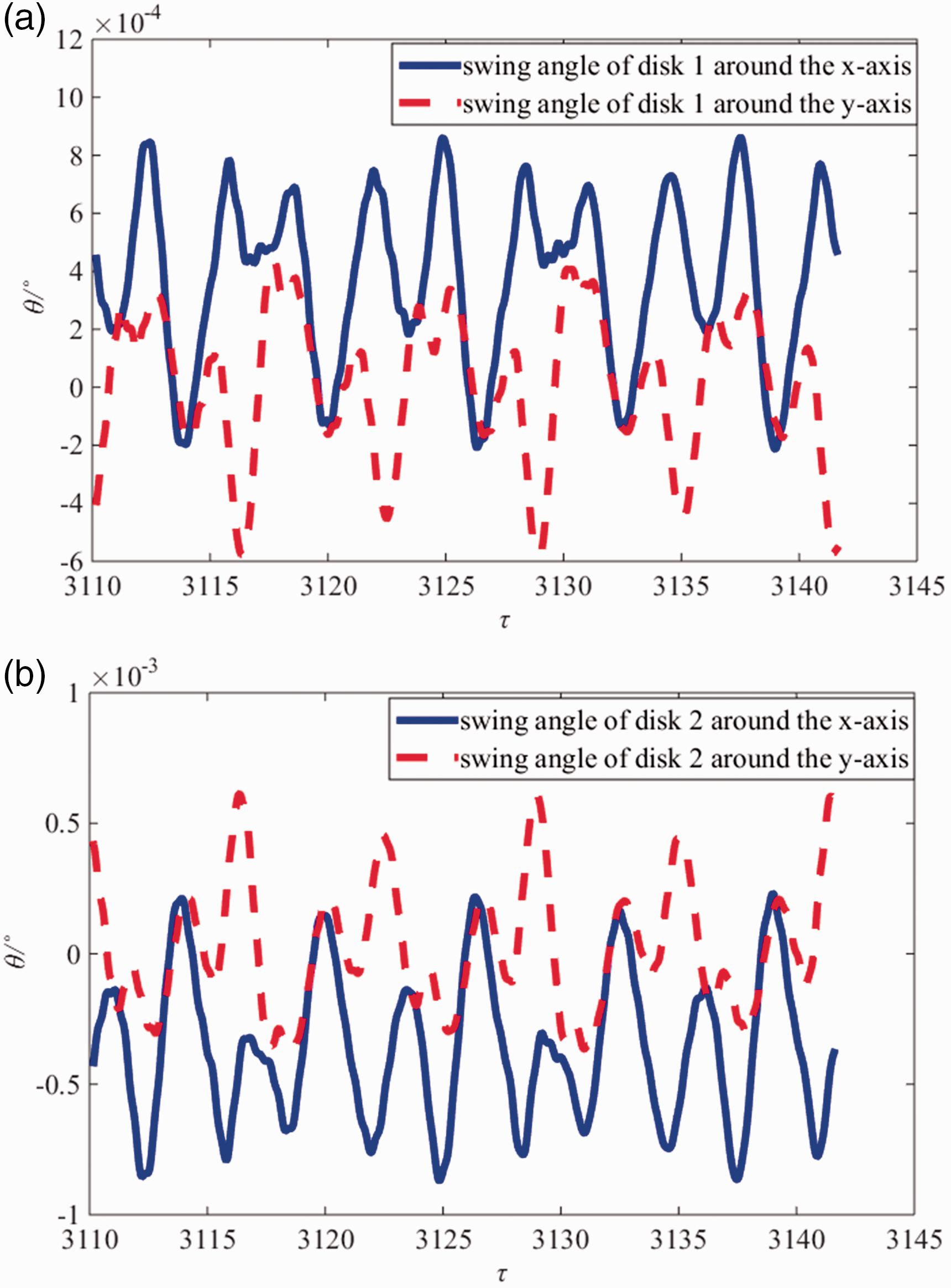
The swing angle of disks 1 and 2 around the x and y axis for
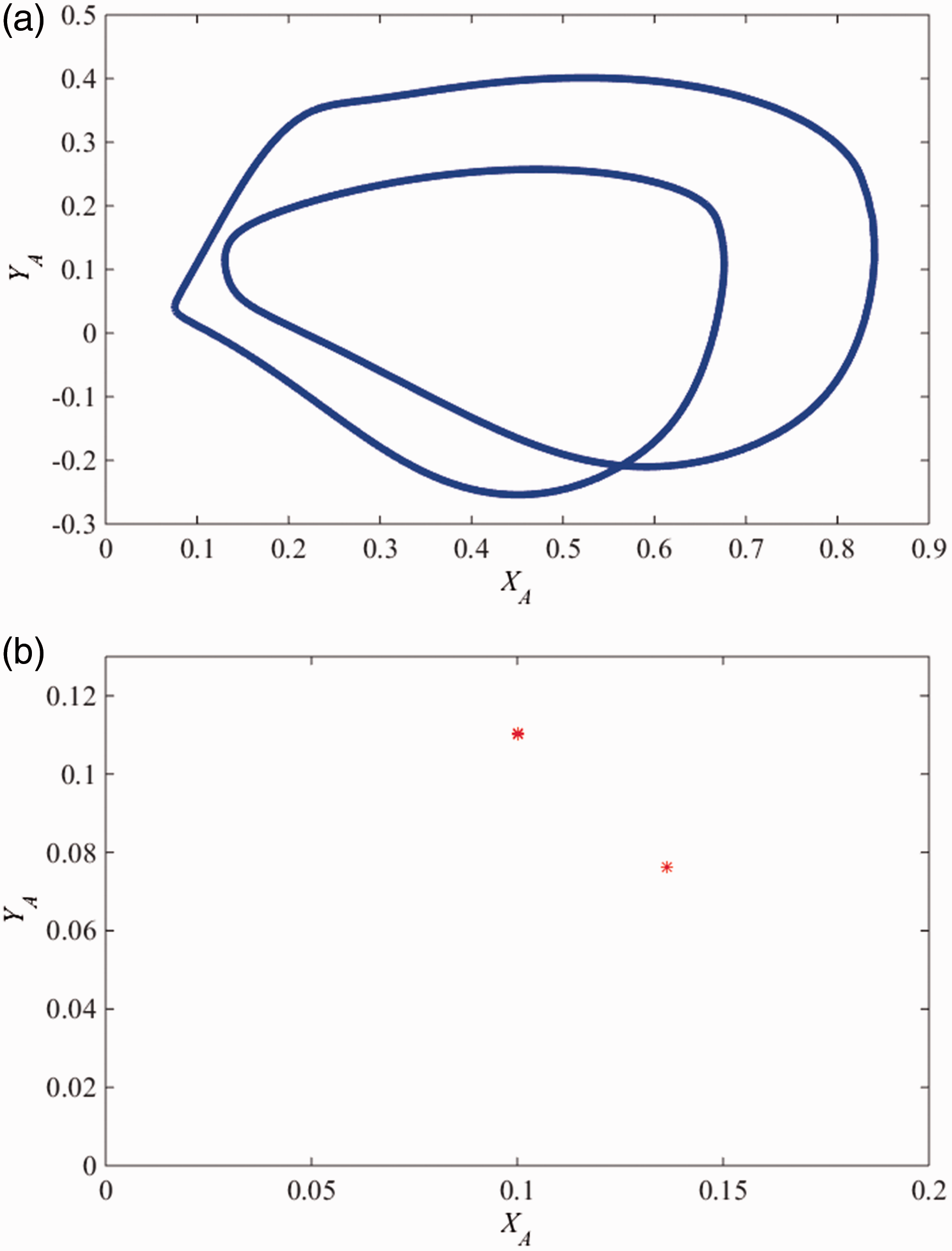
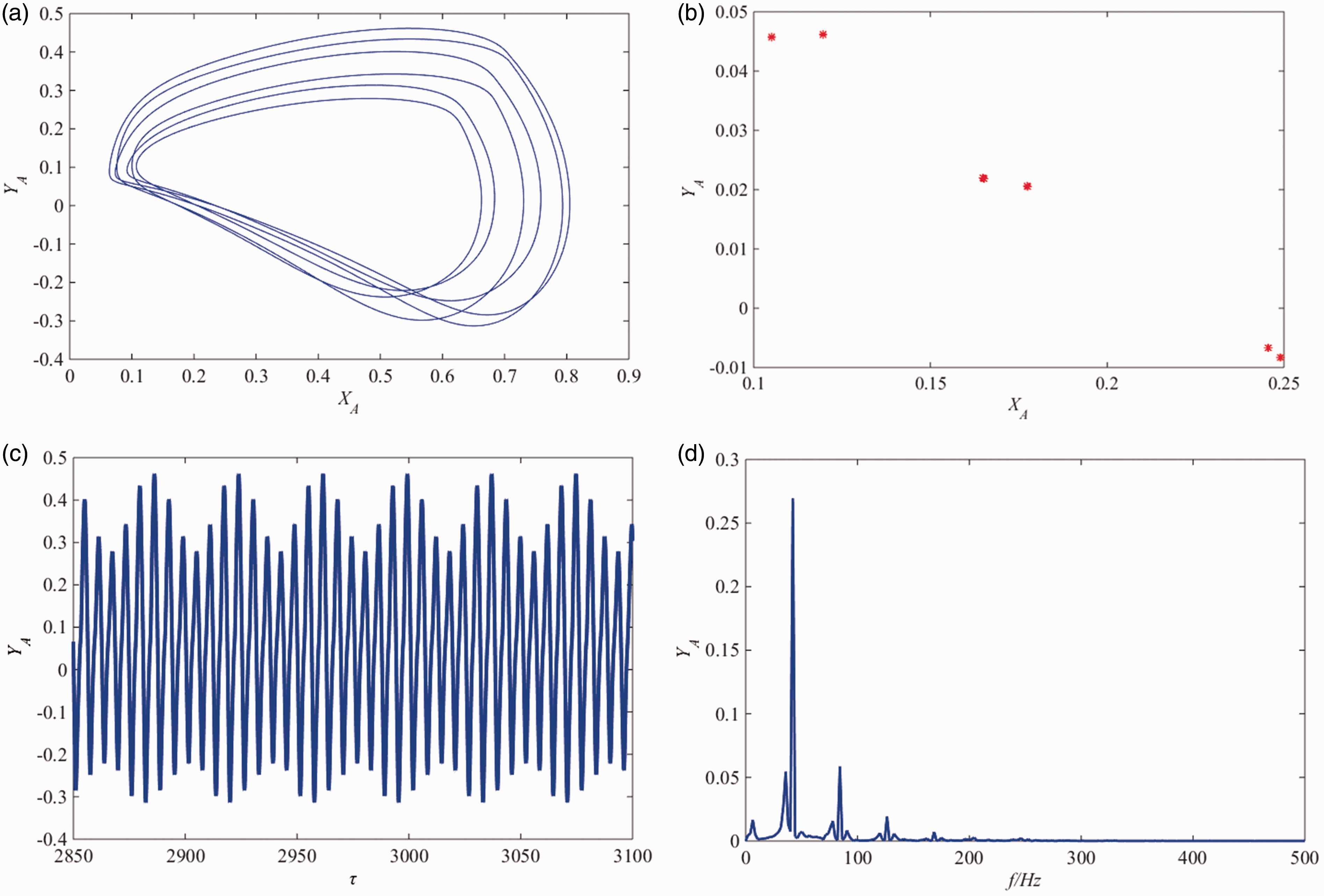
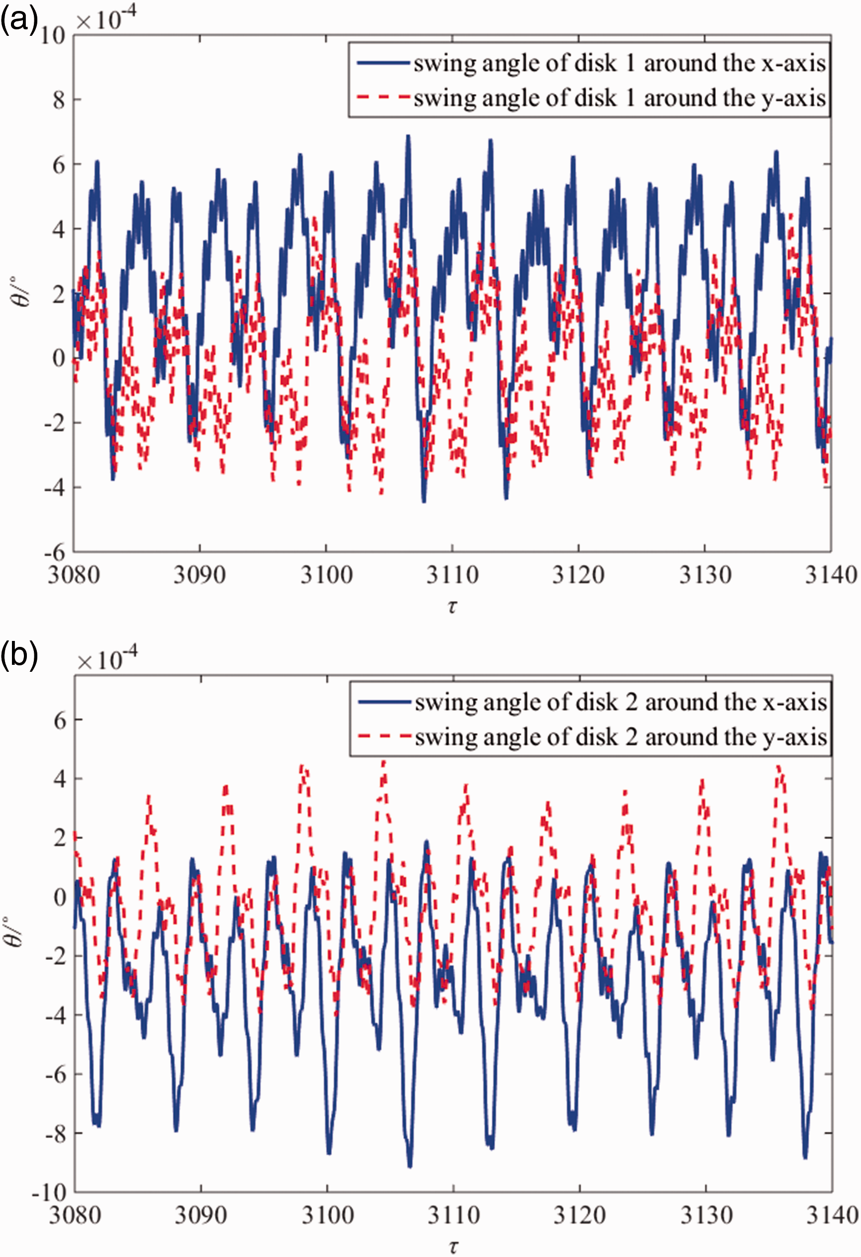
With the increase of the rotating speed, the period-2 motion of the rotor turns to period-4 motion. Figure 14 shows the orbit, Poincaré map, time series and spectrum of the rotor at bearing station when
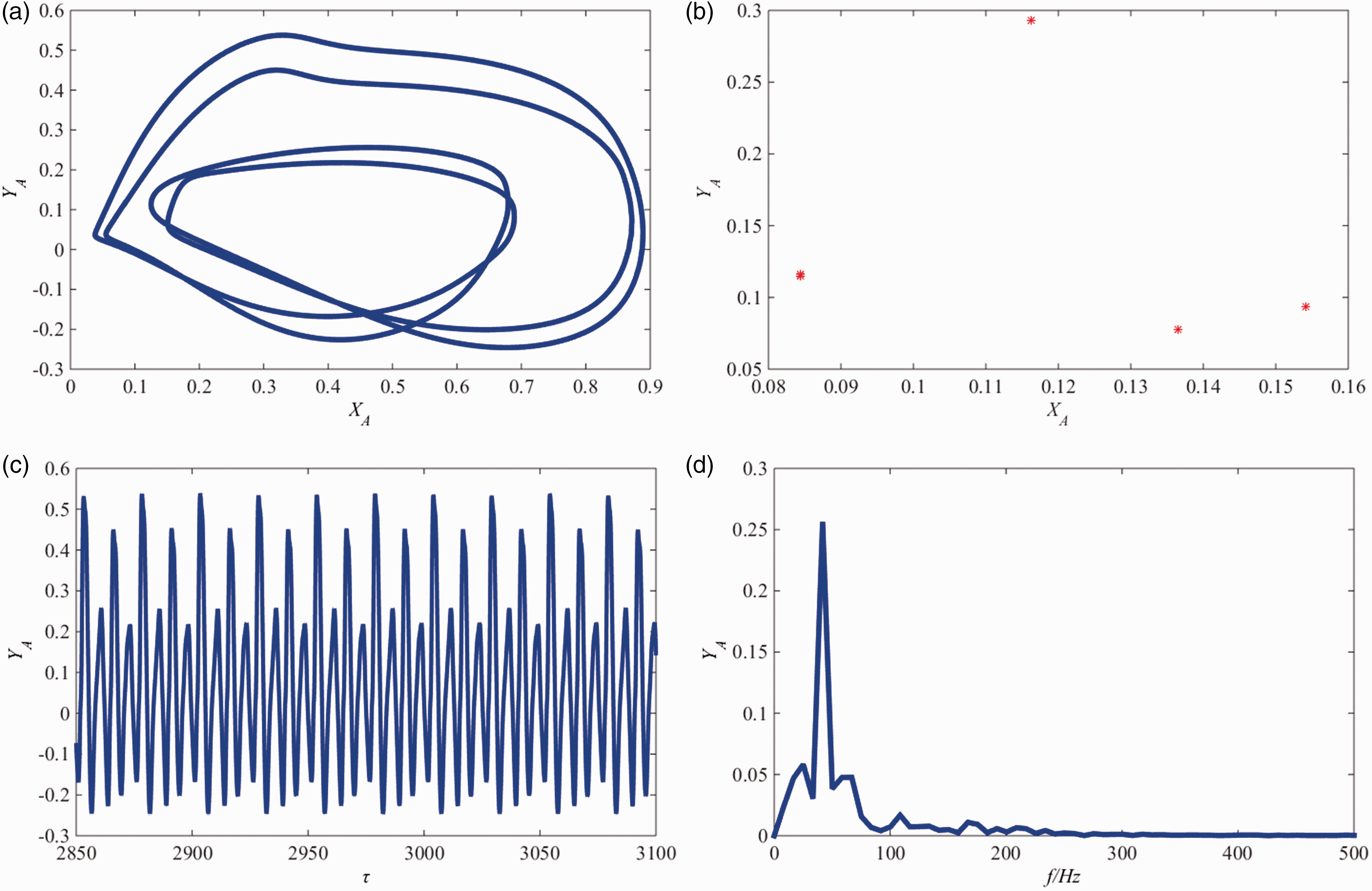
The orbit of rotor, Poincaré map, time series and spectrum of the rotor at bearing station for
The swing angle of disks 1 and 2 around the x and y axis for
For
The orbit, Poincaré map, time series and spectrum of rotor at bearing station for
The swing angle of disks 1 and 2 around the x and y axis for
Taking the dimensionless bending stiffness of the shafts as control parameter
The dimensionless bending stiffness of the shafts contain K11, K22, Kʹ11, Kʹ22. In this section, K11 = K22 = Kʹ11 = Kʹ22 = K. Taking the dimensionless bending stiffness K as control parameter, the dynamics responses of the rod fastening rotor system are investigated when
When the dimensionless stiffness K changes from 3.0 to 6.0, Figure 18 shows the bifurcation diagram of the rotor at bearing station and disk 1station respectively. From Figure 18, it can be seen that the motion types of the rotor system are period-4 motion, period-2 motion, periodic motion, quasi-periodic motion, period-6 motion, quasi-periodic motion, and periodic motion when the dimensionless stiffness K are 3.0, 3.5, 3.8, 4.3, 4.5, 4.7, and 6.0.
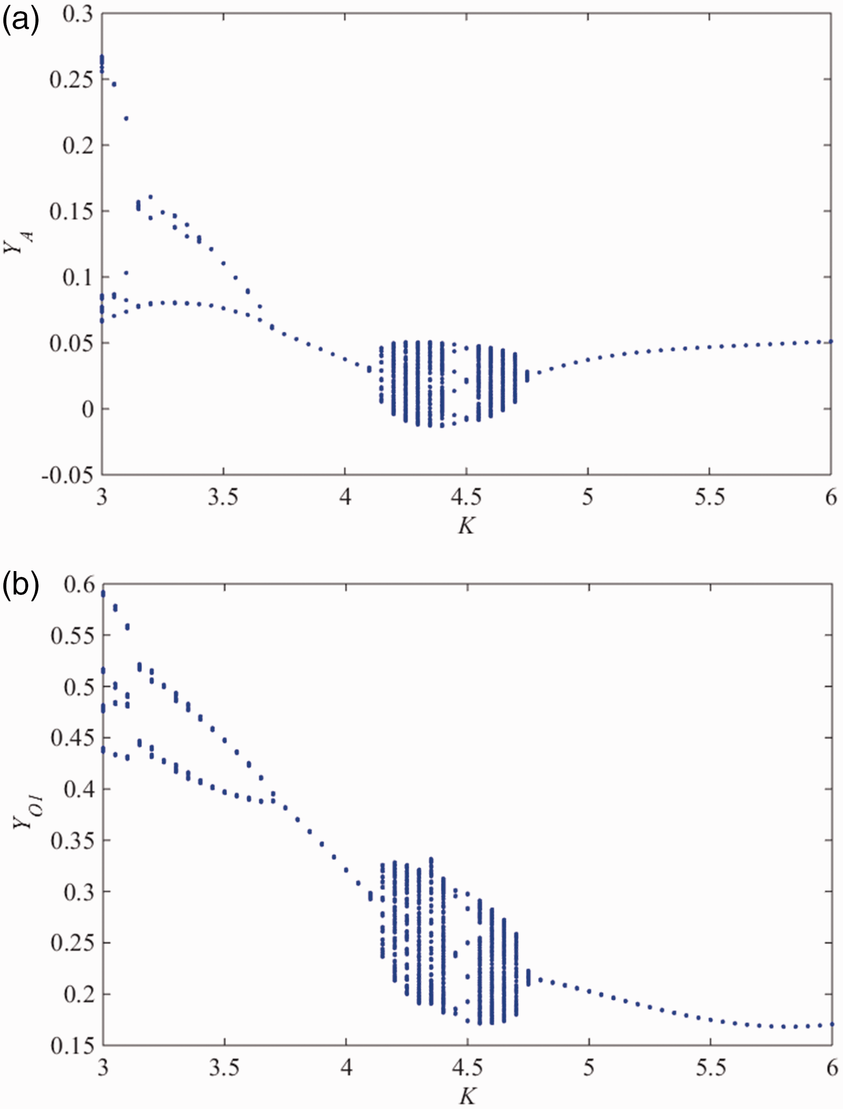
Bifurcation diagram of y versus K at bearing station and disk stations. (a) Bifurcation diagram of y at bearing station; (b) Bifurcation diagram of y at disk 1 station.
When the dimensionless bending stiffness of the shaft is low, the motion of the rotor is period-4 motion. When K = 3.0, the orbit, Poincaré map, time series and spectrum of period-4 motion of the rotor are shown in Figure 14. With the increase of the dimensionless bending stiffness of the shaft, period-4 motion of the rotor turns to a period-2 motion. When K = 3.5, Figure 19 shows the orbit and Poincaré map of the period-2 motion of the rotor.
The orbit, Poincaré map of rotor at bearing station for K = 3.5. (a) The orbit of the journal at bearing station A; (b) Poincaré map.
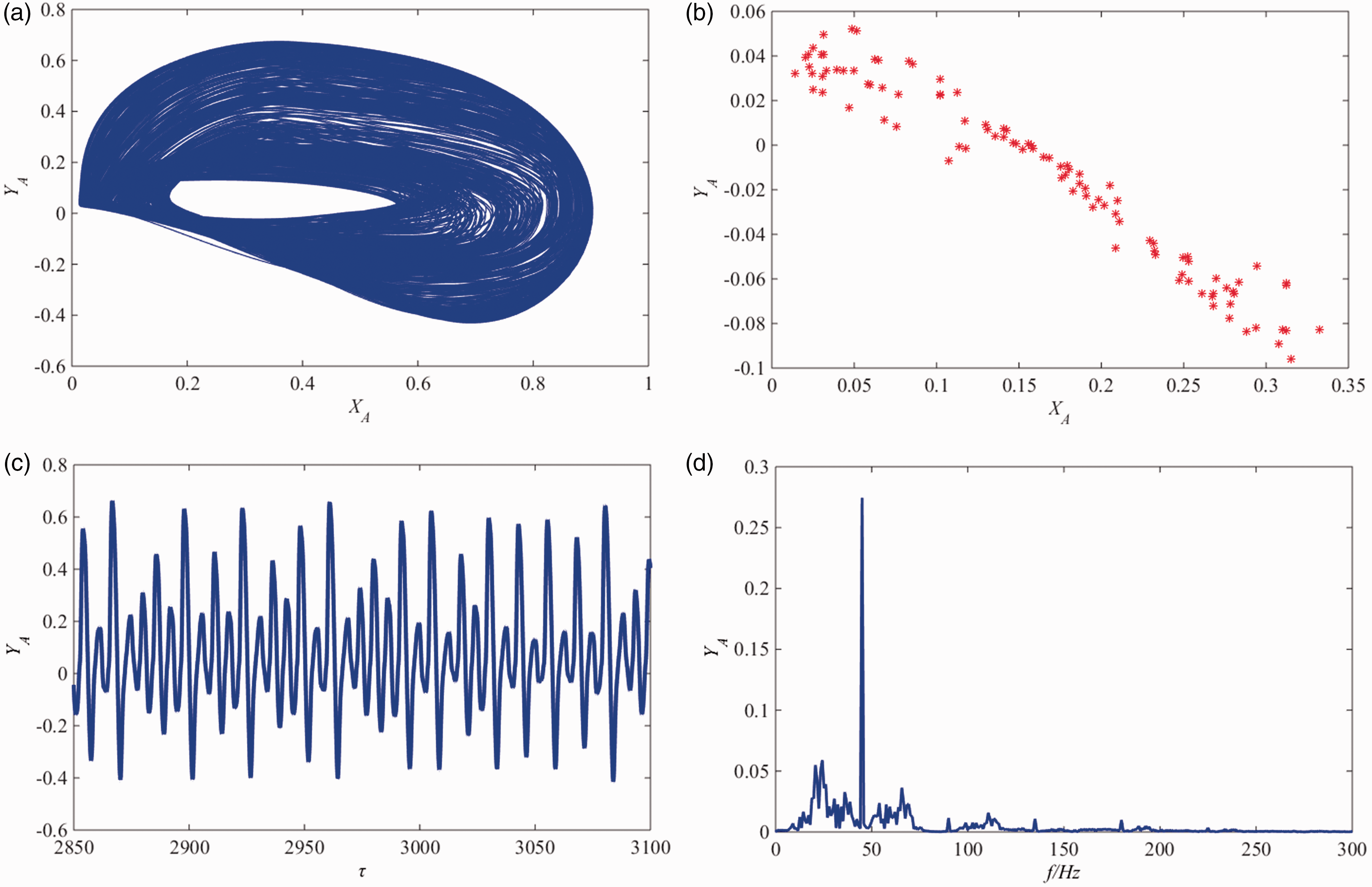
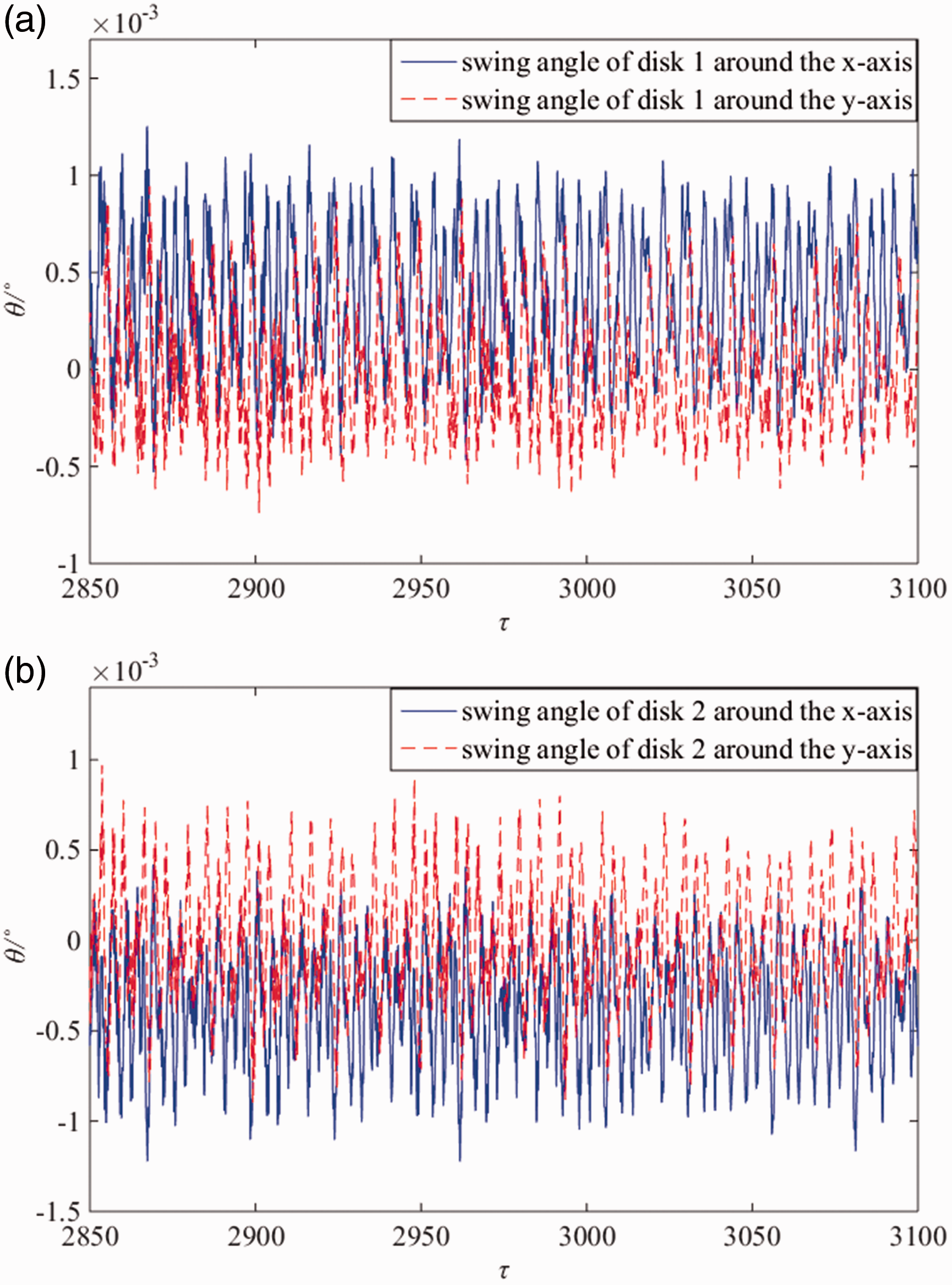
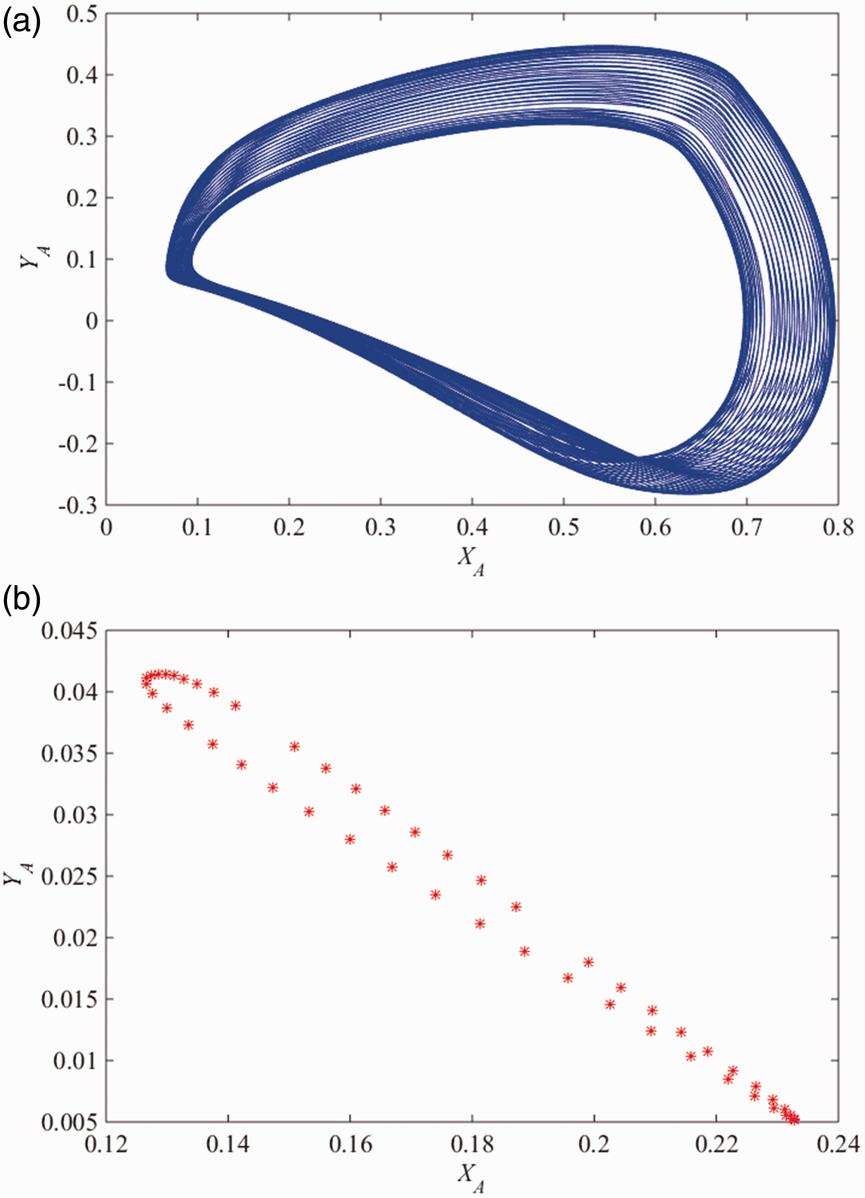
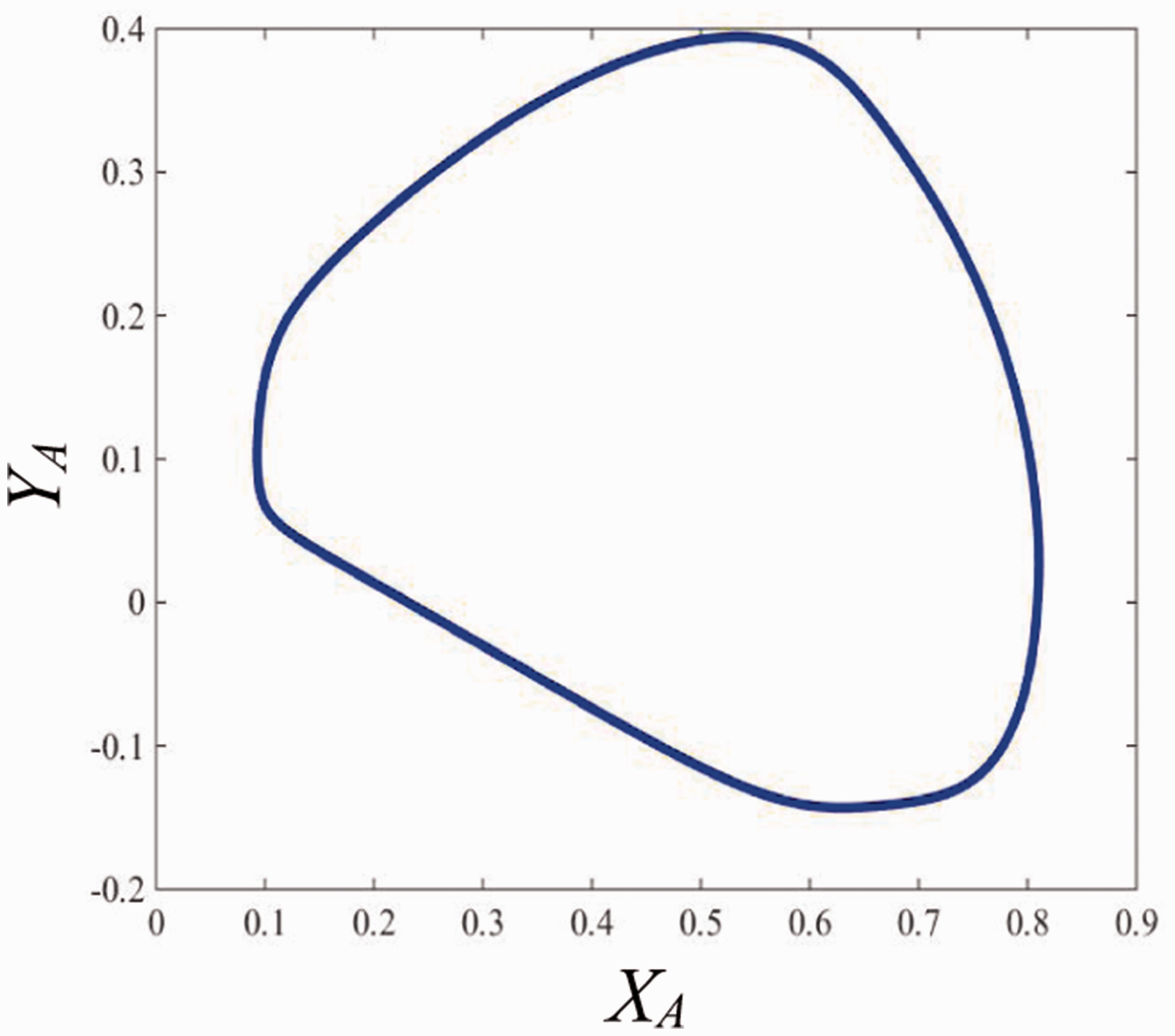
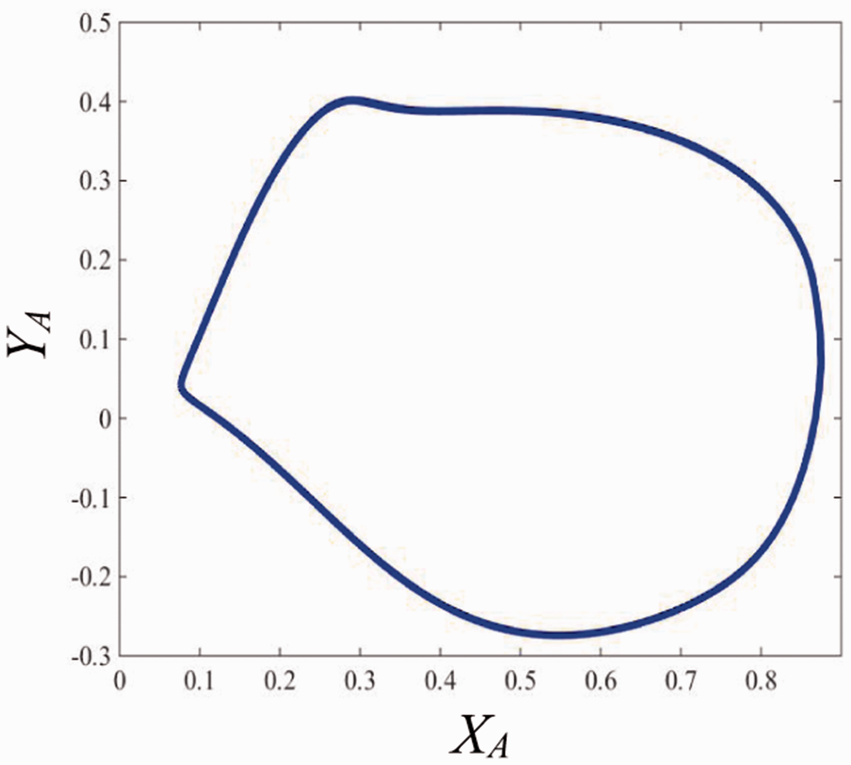
With the dimensionless bending stiffness of the shaft increase continuously, the period-2 motion bifurcates to stable periodic motion. When K = 3.8, Figure 20 shows the orbit of periodic motion of the rotor. Then, the quasi-periodic bifurcation (i.e., the periodic motion turns to quasi-periodic motion) appears with the increase of the dimensionless bending stiffness of the shaft. When K = 4.3, Figure 21 shows the orbit, Poincaré map, time series and spectrum of the rotor. From Figure 21(a), it can be seen that the quasi-periodic orbit is in a bounded region, and the projection of the Poincaré map is a closed curve which is shown in Figure 21(b). From Figure 21(c) and (d), it can be seen that the amplitude of the orbit is irregular, and frequency spectrum contains multiple frequency components. Figure 22 shows the swing angle of the disks, and the swing angle of the disks are irregular.
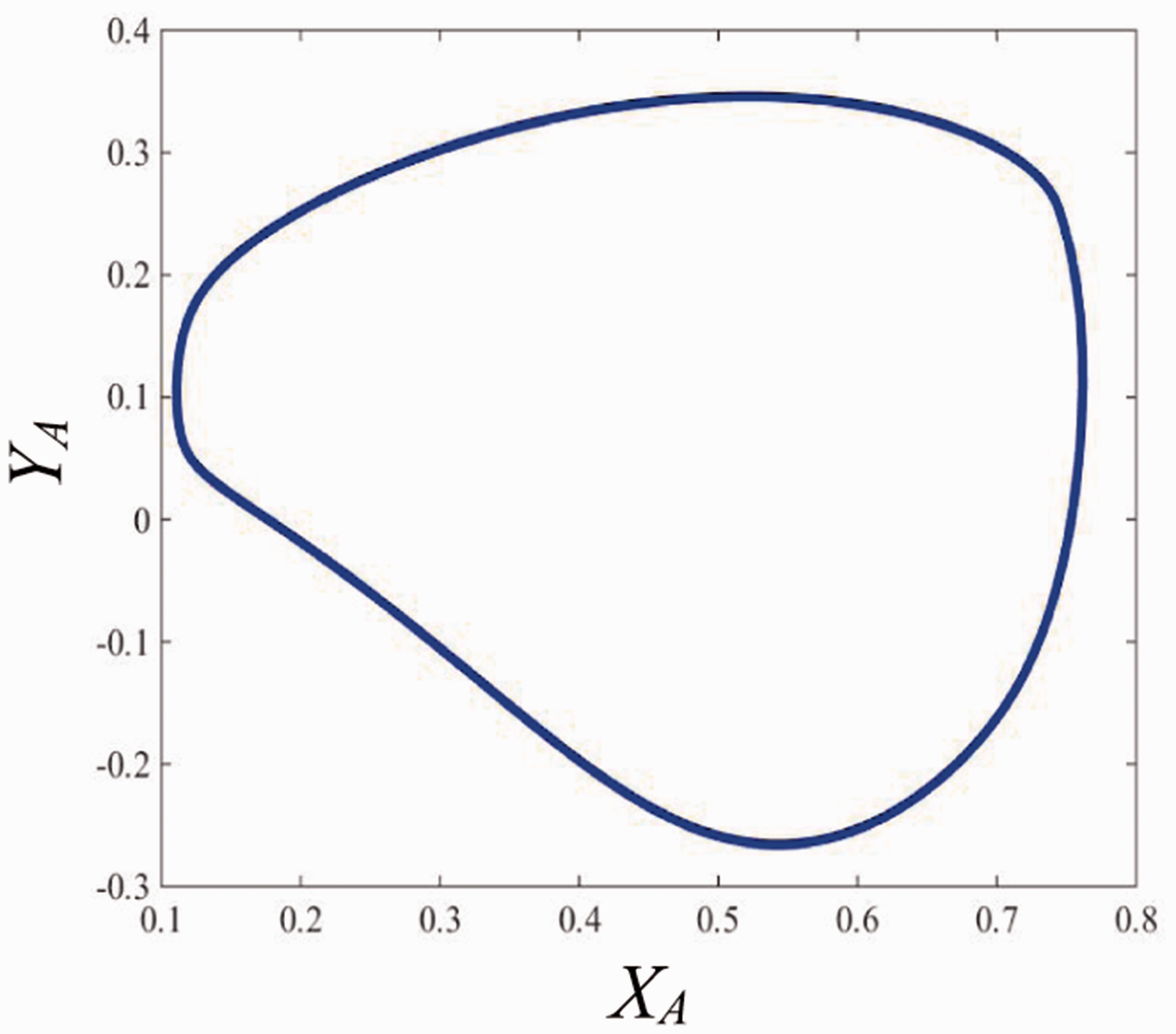
The orbit of rotor at bearing station for K = 3.8.
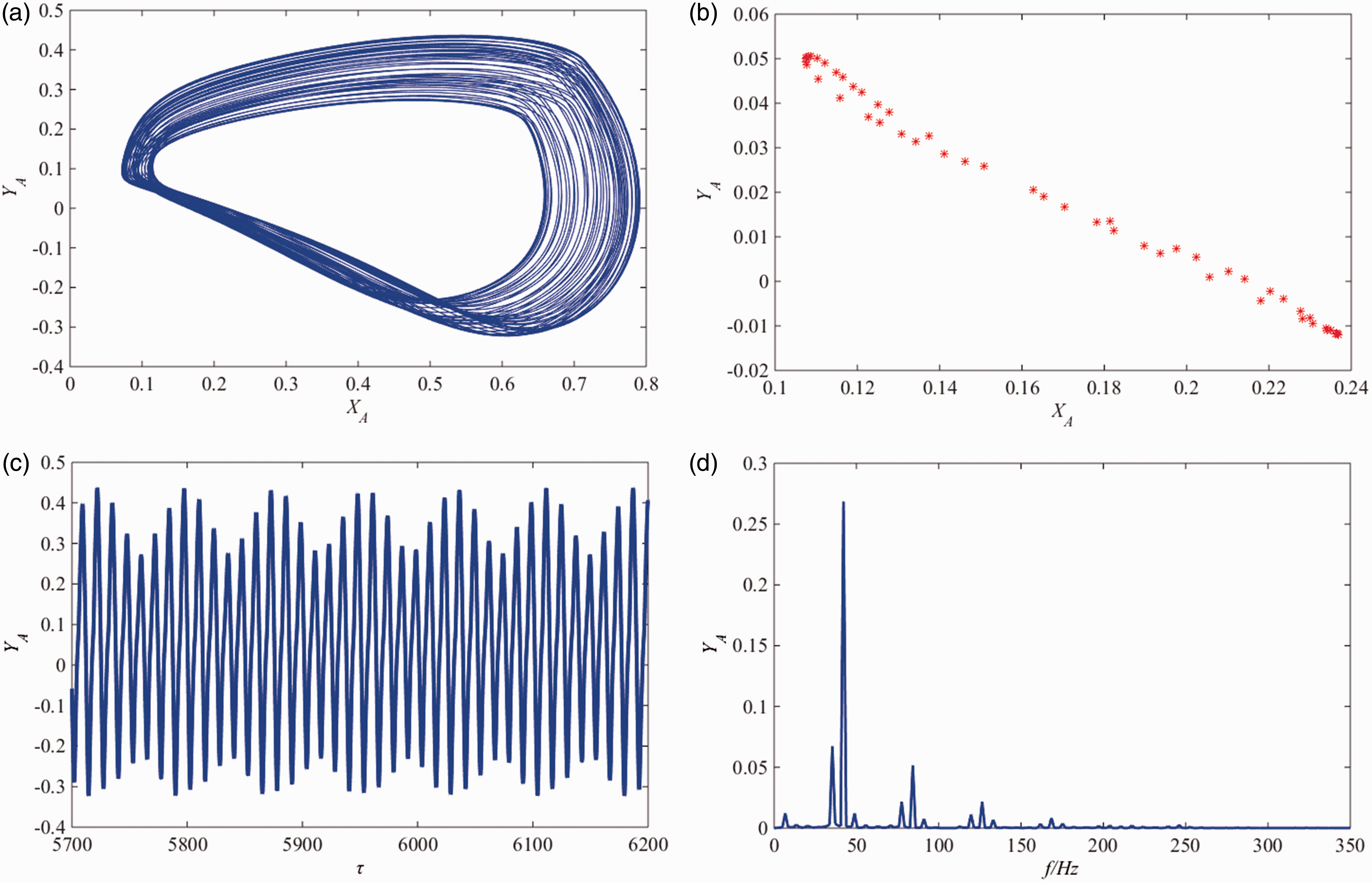
The orbit, Poincaré map, time series and spectrum of the rotor at bearing station for K = 4.3. (a) The orbit of the journal at bearing station A; (b) Poincaré map; (c) Time series (d) The spectrum.
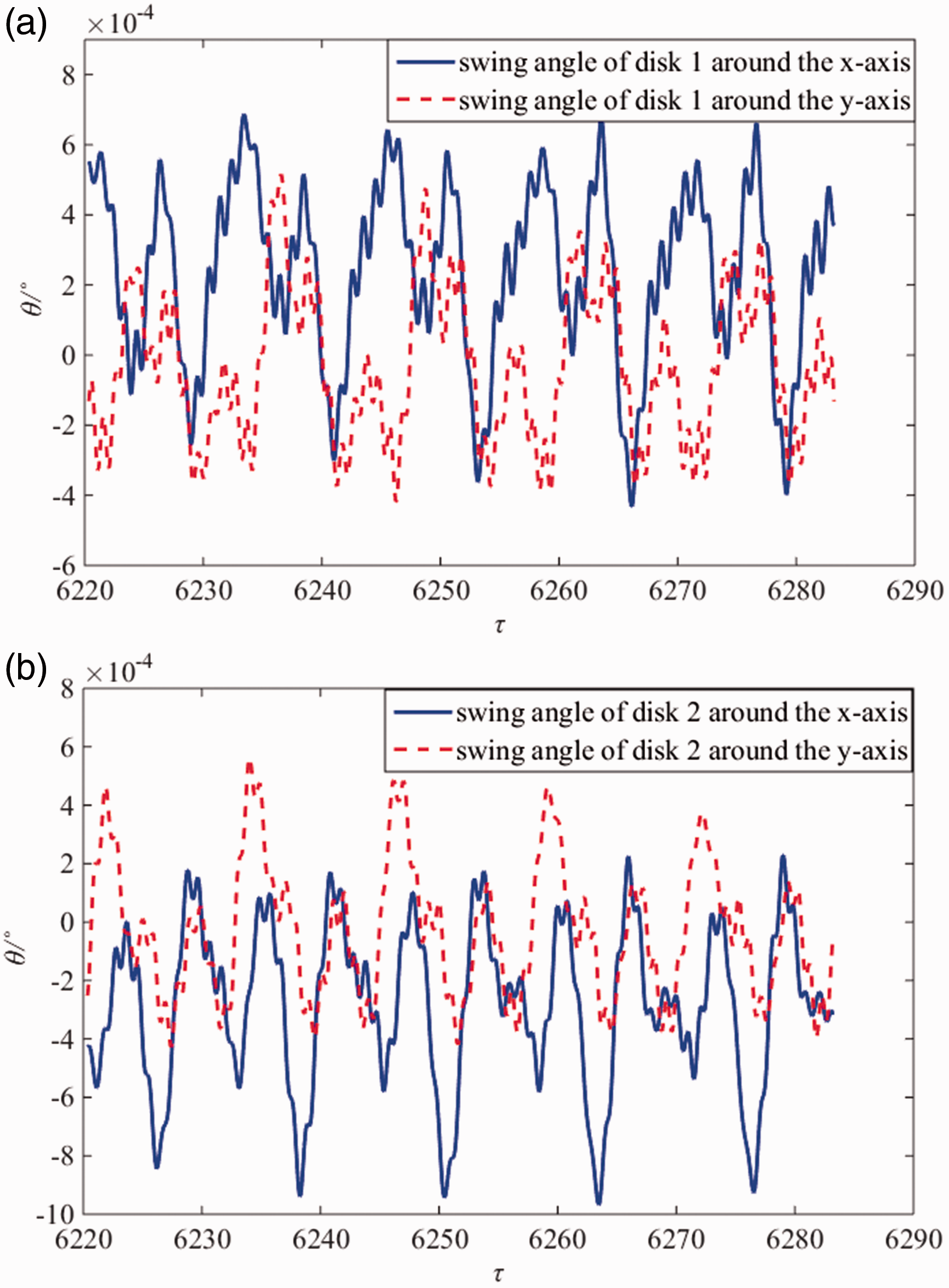
The swing angle of disks 1 and 2 around the x and y axis for K = 4.3. (a) The swing angle of disks 1 around the x and y axis; (b) The swing angle of disks 2 around the x and y axis.
When K = 4.5, Figure 23 shows the orbit, Poincaré map, time series and spectrum of the rotor. From Figure 23(a), it can be seen that a period-6 motion is appeared for the rotor, and the orbit contains six closed curves. Moreover, there are six fixed points in the Poincaré section, as shown in Figure 23(b). From Figure 23(c) and (d), it can be seen that there are multiple amplitudes and frequency components. Figure 24 shows the swing angle of the disks. With the increase of dimensionless bending stiffness of the shaft, the motion of the rotor changed from period-6 motion to quasi-periodic motion, and then, the quasi-periodic motion turns to stable periodic motion. When K = 4.7, Figure 25 shows the orbit, Poincaré map of the rotor. In Figure 25, it can be seen that the orbit of the rotor is in a bounded area, and projection of the Poincaré map is a closed curve. Figure 26 shows the orbit of the rotor when K = 6, and the orbit of the rotor is a closed curve.
The orbit, Poincaré map, time series and spectrum of the rotor at bearing station for K = 4.5. (a) The orbit of the journal at bearing station A; (b) Poincaré map; (c) Time series; (d) The spectrum.
The swing angle of disks 1 and 2 around the x and y axis for K = 4.5. (a) The swing angle of disks 1 around the x and y axis; (b) The swing angle of disks 2 around the x and y axis.
The orbit, Poincaré map of rotor at bearing station for K = 4.7. (a) The orbit of the journal at bearing station A; (b) Poincaré map.
The orbit of rotor at bearing station for K = 6.0.
Taking the dimensionless eccentricity of the disks as control parameter
Taking the dimensionless eccentricity of the disks as control parameter, the dynamic behaviors of the rotor system are investigated. In the investigation, the dimensionless rotating speed
Figure 27 shows the bifurcation of the rotor at the bearing and disk 1 station. From Figure 27, it can be seen that the rotor will exhibits quasi-periodic motion, periodic motion, period-2 motion, period-4 motion, period-2 motion, and periodic motion with the increase of the dimensionless eccentricity.
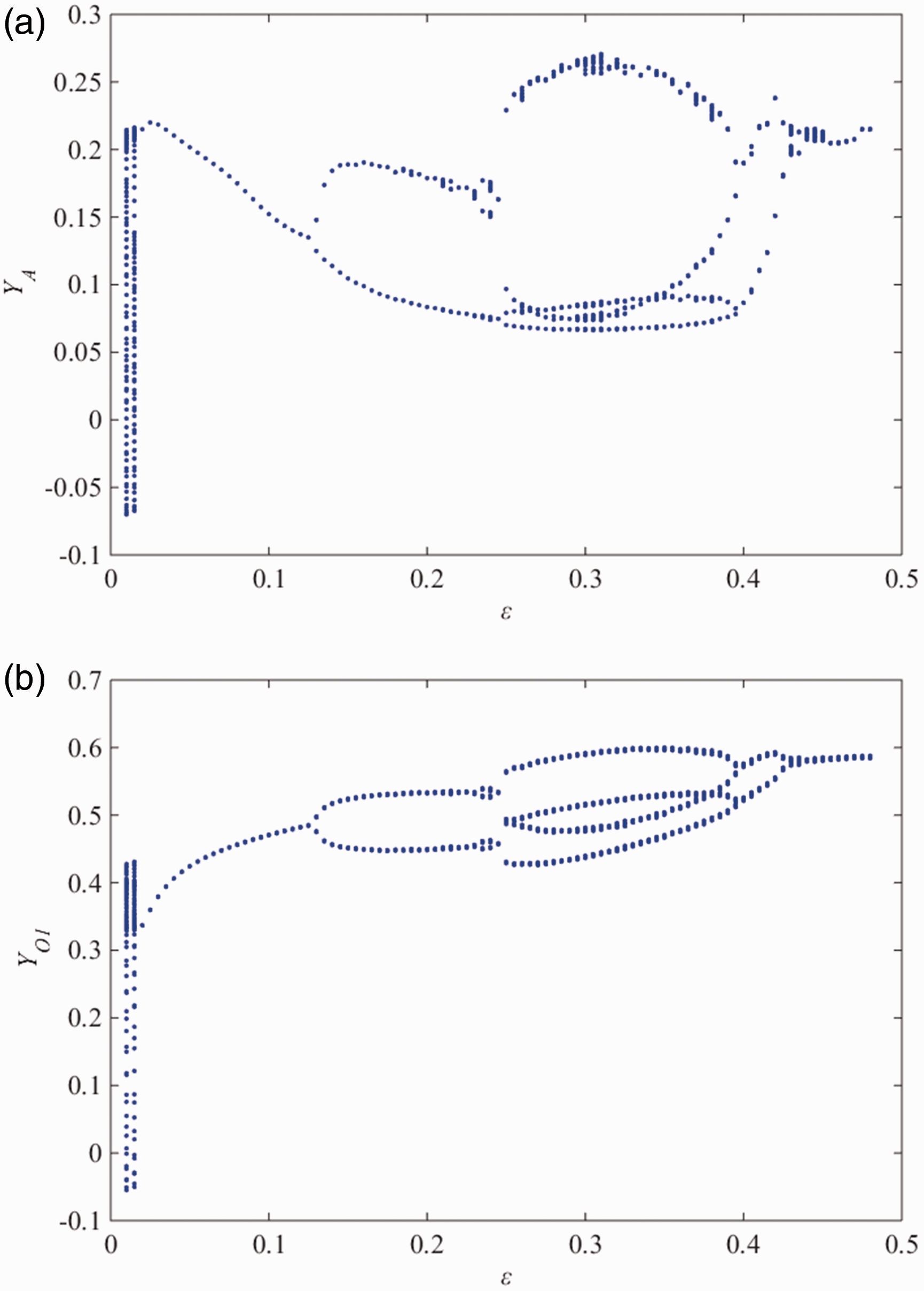
Bifurcation diagram of y versus ε at bearing station and disk stations. (a) Bifurcation diagram of y at bearing station; (b) Bifurcation diagram of y at disk 1 station.
When the dimensionless eccentricity of the disks is very low, the motion of the rotor is quasi-periodic motion. Figure 28 shows the orbit and Poincaré map of the rotor at the bearing station for ε = 0.01. Then, quasi-periodic motion will turn to periodic motion. When ε = 0.08, Figure 29 shows the periodic orbit of the rotor at the bearing station. With the increase of the dimensionless eccentricity of the disks, the periodic motion bifurcates to a period-2 motion. When ε = 0.15, Figure 30 shows the orbit and Poincaré map of the rotor at the bearing station. The bifurcation phenomenon occurs again when the dimensionless eccentricity increases continuously, and the period-2 motion will turn to period-4 motion. When ε = 0.3, Figure 14 shows the calculating results. The period-4 motion bifurcates to period-2 motion when the dimensionless eccentricity increase continuously. Figure 31 shows the orbit and Poincaré map of the rotor at the bearing station when ε = 0.42. Then, the motion of the rotor will turn to stable periodic motion with the increase of the dimensionless eccentricity of the disks. Figure 32 shows the orbit of the rotor at bearing station when ε = 0.46.
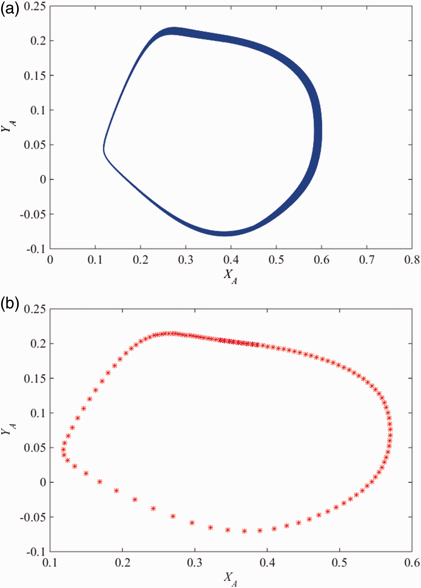
The orbit, Poincaré map of rotor at bearing station for ε = 0.01. (a) The orbit of the journal at bearing station A; (b) Poincaré map.
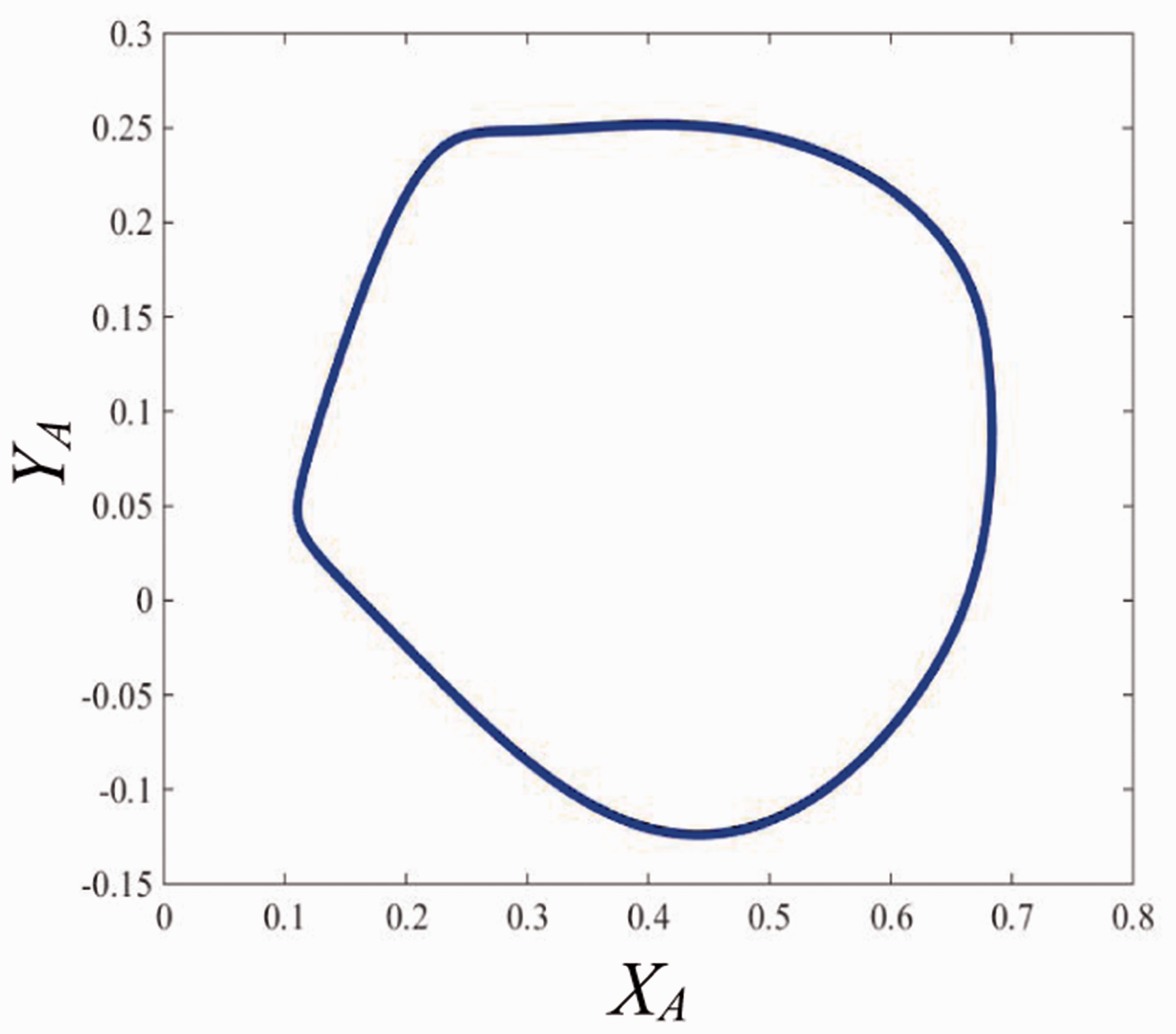
The orbit of rotor at bearing station for ε = 0.08.
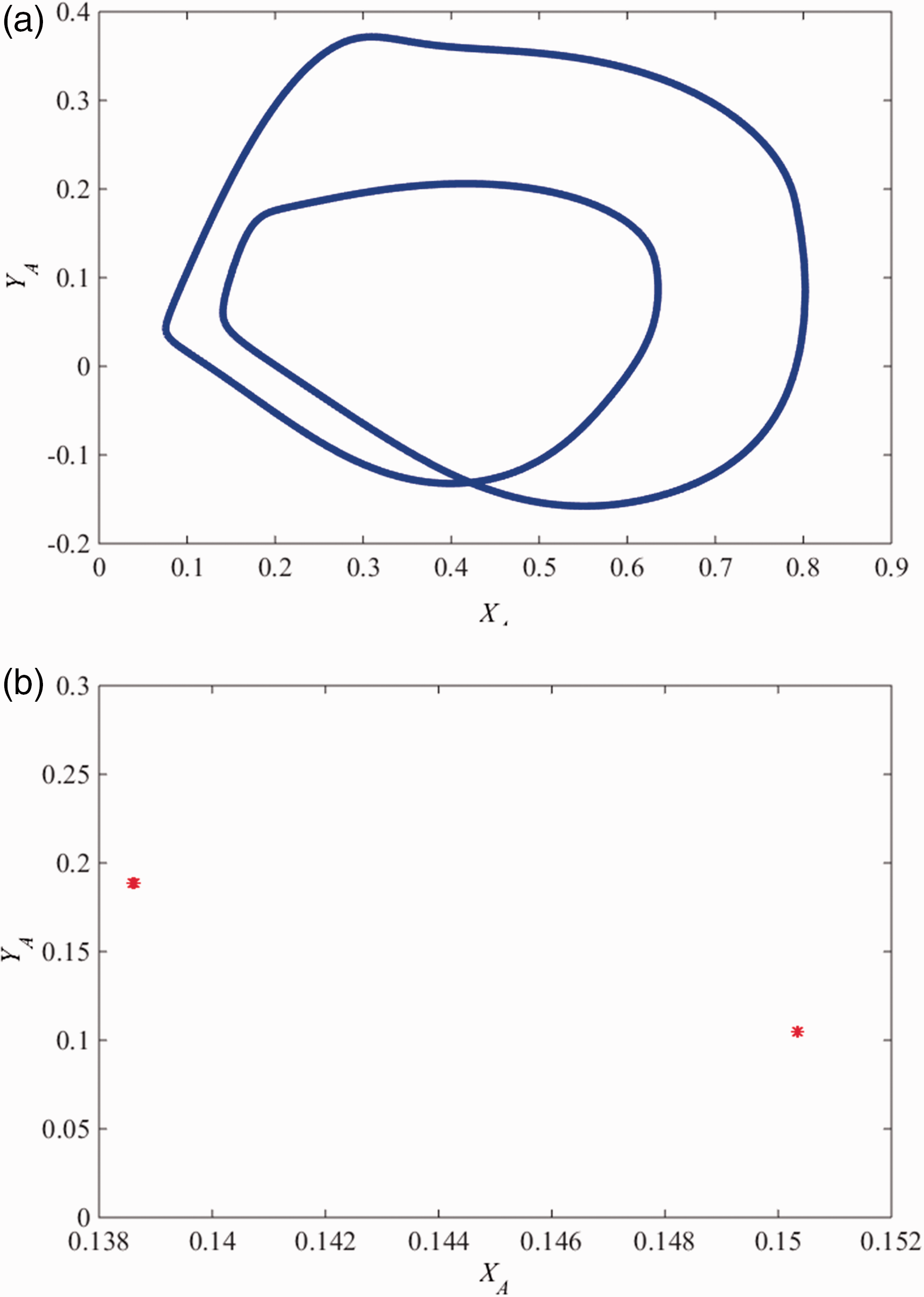
The orbit, Poincaré map of rotor at bearing station for ε = 0.15. (a) The orbit of the journal at bearing station A; (b) Poincaré map.
The orbit, Poincaré map of rotor at bearing station for ε = 0.42. (a) The orbit of the journal at bearing station A; (b) Poincaré map.
The orbit of rotor at bearing station for ε = 0.46.
Taking the dimensionless contact stiffness of the disks as control parameter
Letting Kb=KR, the influence of the dimensionless contact stiffness Kb and KR on the dynamics of the rod fastening rotor bearing system is studied. The parameters are the same as the section “Taking the dimensionless speed as control parameter.” For Kb=KR=0.1, 0.7, 2, 20, Figure33(a) to (d) show the bifurcation diagram at bearing station. From Figure 33, it can be seen that the types of the motions of the rotor system are similar when
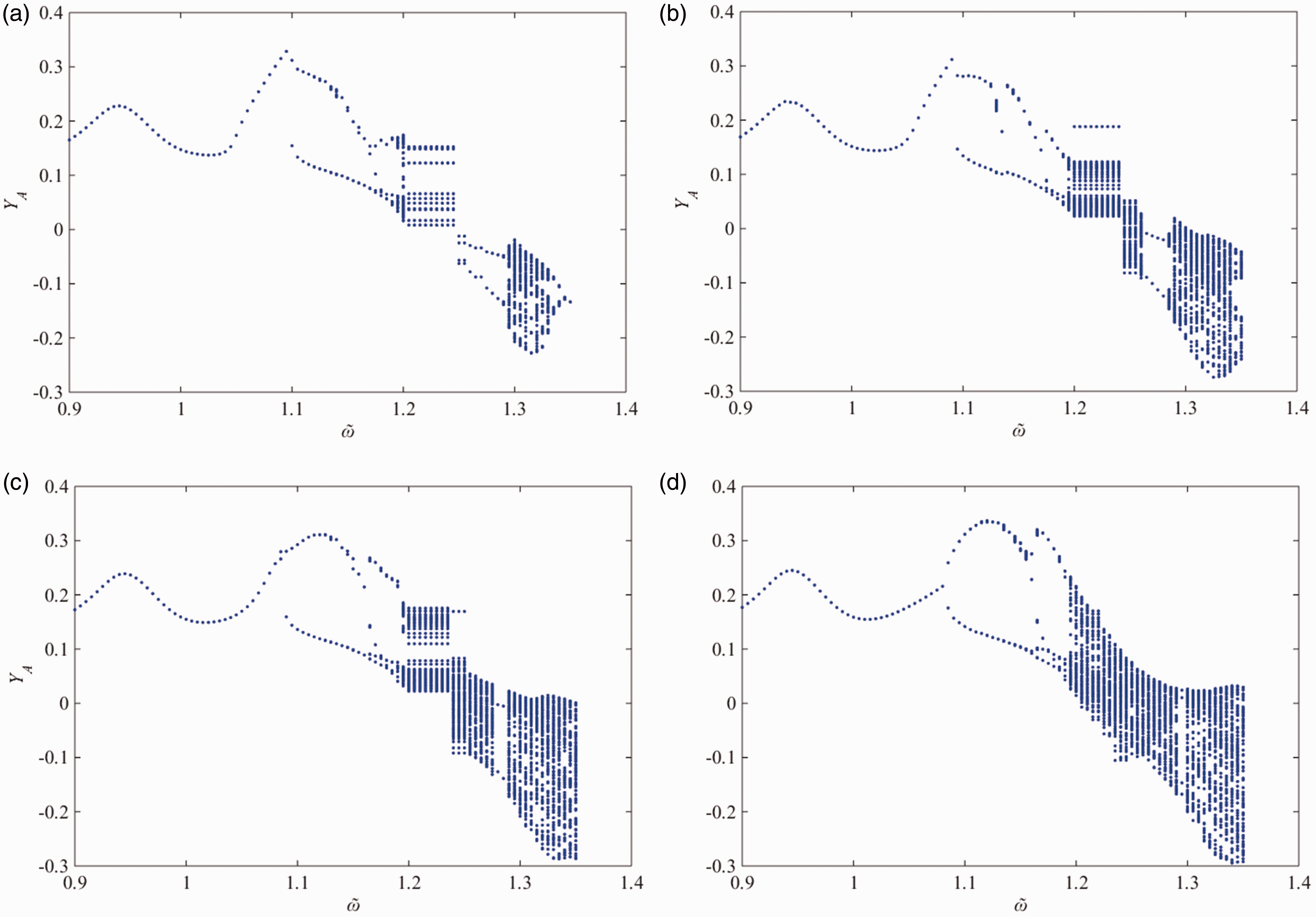
Bifurcation diagram of y versus
At the same time, it is found that the rotor collides with the wall of the bearing in the speed range of 1.21–1.245 when Kb=KR=0.1. The speed range shrinks gradually with the increase of the dimensionless contact stiffness, and the range disappears completely when Kb=KR=20. For Kb=KR=0.1 and
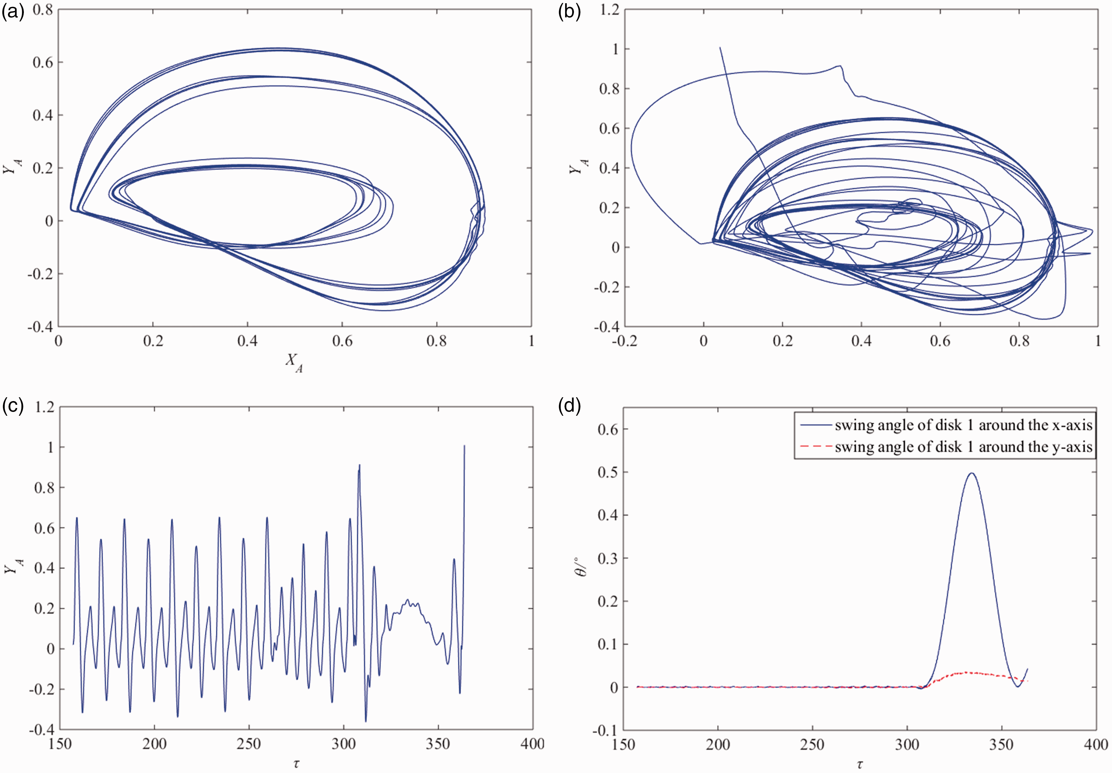
The orbit, time series of the rotor at bearing station and the swing angle of disks 1 around the x and y axis for Kb=KR=0.1,
Conclusions
In this study, to investigate the dynamic behaviors of a rod fastening rotor. A motion model of rod fastening rotor is developed by considering the contact effect and gyro effect of the disks. An approximate analytical solution of the oil film force for the supporting bearing of the rotor is proposed based on the method of separation of variables and Sturm–Liouville theory, and the Newmark method is improved to solve the motion model of the rotor bearing system. The main results are as follows: The proposed approximate analytical solution can solve the oil film force of the bearing fast, and the results calculated by the proposed approximate analytical solution agree well with the results calculated by the finite difference method. Moreover, compared with the Newmark method, the improved Newmark method has high precision by compensating the disturbance error, and the improved Newmark method has higher calculation efficiency than Runge–Kutta method. Based on the approximate analytical solution of the oil film force and the improved Newmark method, the dynamics behaviors of the rod fastening rotor system and the integral rotor system are studied. The results indicate that the rod fastening rotor system is more stable than the integral rotor system. Taking the dimensionless rotating speed, bending stiffness of the shaft and the eccentricity of the disks as control parameter, the rod fastening rotor system exhibits rich and complex nonlinear dynamic behaviors. Furthermore, the influence of the contact stiffness of the disks on the dynamic motion of the rotor system is analyzed. The result indicates that the contact stiffness of the disks has great effect on the dynamic behaviors of the rotor system when the rotor operates under non-periodic motion state. Meanwhile, a large swing angle will be observed for the disks when the contact stiffness is inappropriate, and it will consequently result in collision between the rotor and bearing.
Footnotes
Declaration of Conflicting Interests
The author(s) declared no potential conflicts of interest with respect to the research, authorship, and/or publication of this article.
Funding
The author(s) disclosed receipt of the following financial support for the research, authorship, and/or publication of this article: This work was supported by the Natural Scientific Research Program of Shaanxi Province of China (No. 2019JQ-928), Research Program of Weinan of Shaanxi Province of China (Nos.2016KYJ-1–2, 2018-ZDYF-JCYJ-60), Research Program of Shaanxi Railway Institute of China (No. KY2018-53).