Sage Journals: Discover world-class research

Abstract

This paper presents the optimal design of in-plant logistics in manufacturing. Owing to rising energy costs and the supply-demand imbalance leading to price competition, resulting in a sharp decline in profit, business management is facing a severe test, especially heavy industry. In practice, the important decision-making in C Company has relied on expert experience and existing knowledge, the lack of systematic thinking, and technology applications, resulting in a waste of logistics costs. Therefore, a study on the application of genetic algorithms to optimize steel mill factory by-product transport and logistics is presented herein. The aim is to solve the bottleneck of traditional decision-making in order to achieve the goal of optimizing transportation logistics decision-making via artificial intelligence. In defining the problem, the model of the steel mill factory by-products transport and logistics is constructed through in-plant route information, vehicle routing systematization and consideration of the transport demand frequency. The modified variable length chromosome ending technique and bi-level genetic algorithm are used to effectively solve the problem of different zoning transportation on double layer genetic algorithm application. The results show that the total transport time is slightly better than the existing results.

Keywords

By-product genetic algorithm artificial intelligence

Introduction

Steelmaking is an essential industry in many advanced and developing countries. Several fundamental steel products, including steel plates, steel strips, rolled steels, etc., made by the steelmaking manufacturers have been utilized in the creation of various basic infrastructures in modern cities. However, various by-products are also being produced during steelmaking, such as scrap metal, steel rust skin, etc. If those by-products are not dealt with properly by recycling and reuse processes, serious environmental pollution will result. Therefore, the recycling and reuse of the by-products are critical issues in every steel mill due to the cost and environmental problems. To address these problems, the steelmaking by-products should be categorized, packed in containers, and then transported by the recycling vehicles to the recycling stations. In other words, the demand for by-product transport and logistics efficiency is essential in steel mills.

Generally, the features of the by-products are heavy weight, large size, irregularity, and high temperature. Most of the by-products in the steel mills are filled into containers and transported by vehicles such as shown in Figure 1, where the containers are located according to the type of by-products. Due to the features of steel mill by-products, large fuel consumption is required to transport the by-products. Moreover, it is better to classify the by-products according to the variables of size, material, weight, etc. In addition, the zoning of the container should also be categorized. Hence, the zoning plan and traveling path of the by-products transport and logistics need to be strictly considered and designed for reducing the traveling time, cost, and environmental pollution. The issues mentioned above are more complicated than the conventional traveling salesman problem (TSP) and vehicle routing problem (VRP); even the demands of the zoning problem (ZP) should be considered in the transport and logistics of steel mill by-products.

Figure 1.

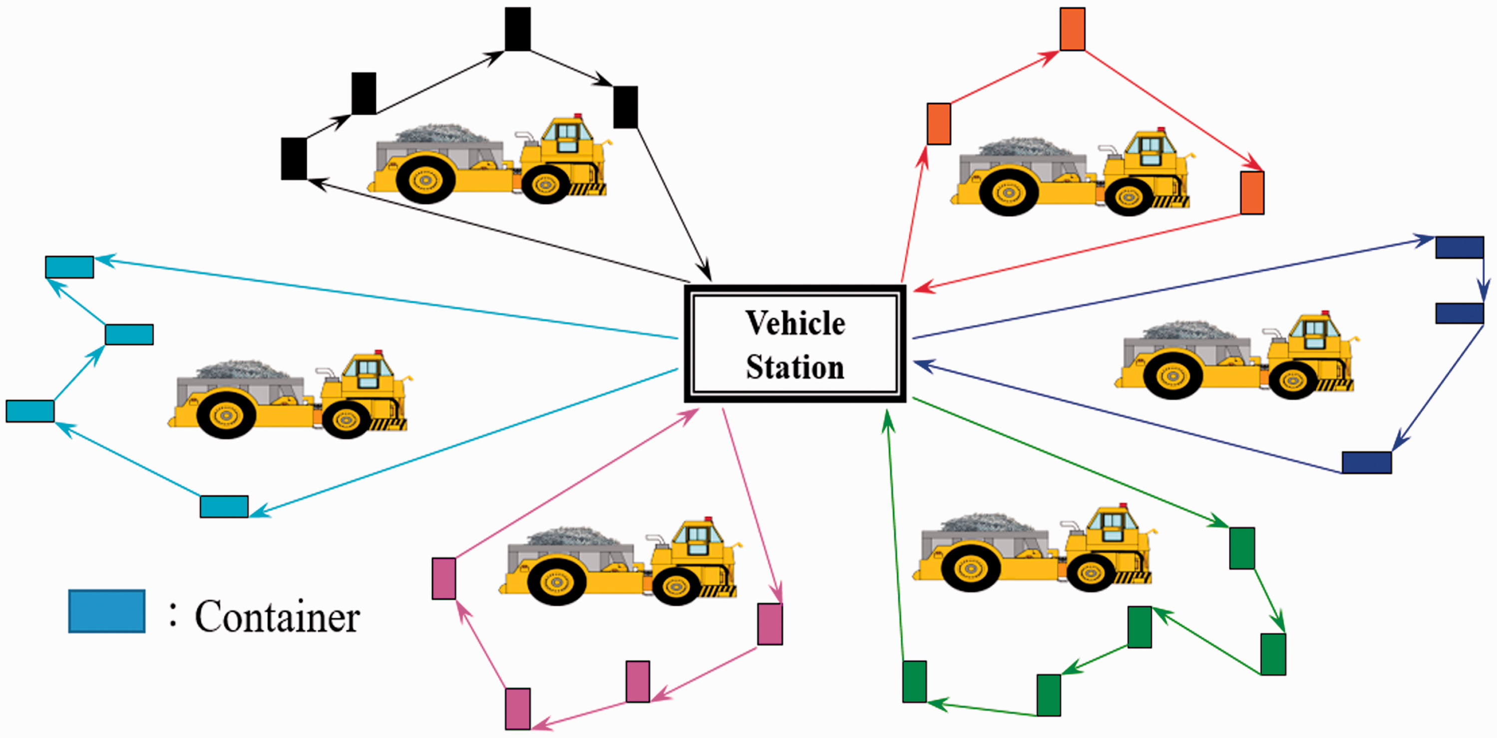
Transport flow of loading container.

A traditional TSP had been discussed with a single station, a single transportation route and several demand points (customer), such as shown in Figure 2(a)^1,2 where the square pattern indicates a station, the circle pattern presents the demand points (customer), and the arrow-line shows the transportation route. Meanwhile, the limitation of the container was not considered during the transportation process in TSP. In other words, a TSP path is a minimum distance problem under a single salesman starting from a station and going back to the origin station after delivering goods to every demand point (customers). However, the multi-transportation routes with several demand points (customers) according to the capacity constraints of the container are integrated into the VRP, as illustrated in Figure 2(b).³ To solve the VRP, the following seven strategies were discussed:⁴ (1) cluster-first route-second, (2) route-first cluster-second, (3) savings or insertion, (4) improvement and exchange, (5) mathematical programing approaches, (6) interactive optimization, and (7) exact procedure. Then, the random and stochastic VRP was presented⁵ based on those strategies in which customer demand is unpredictable. Obviously, a VRP is more complicated than a TSP.

Figure 2.

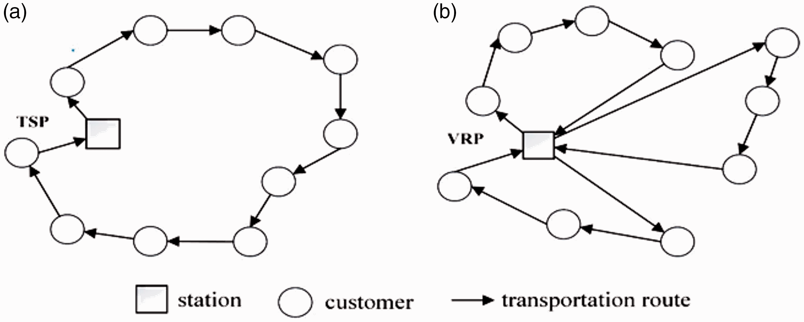
Transportation routes of (a) TSP and (b) VRP.

Furthermore, a conventional VRP belonged to the optimization of the NP-Hard (Non-deterministic Polynomial-time Hard), such as the application of geographically scattered customers to be served by a fleet of vehicles, and the hybrid genetic algorithm (GA) for the problem had been presented.⁶ Since the GA can be applied to various types of optimization problems, the optimal design based on the GA was investigated for the by-product transport and logistics in this study. Additionally, due to the transport and logistics of the by-products in steel mills being a hybrid issue of TSPs, VRPs and ZPs, the optimal design of ZP needed to be investigated.

To address a ZP, integer programming for a bin packing problem with time windows was discussed.⁷ The transportation cost can be reduced around 23% per month and the scheduling time can be reduced about 67%. Moreover, overtime of manual scheduling can be reduced about 50% per day. Furthermore, the fixed and flexible zoning strategies for parcel distribution in uncertainty environments had been proposed.⁸ From the elastic partitioning strategy, the total transport mileage of the customer groups near the station is shortened by 7.2% compared with the fixed partitioning strategy, and the calculation solution time is the shortest compared with other models. The multi-zone multi-trip VRP with time windows was then conducted,⁹ which mainly considered a two-tier city logistics distribution system. Previous studies have shown that transport and logistics will be divided into a number of areas of responsibility under the effective reduction of transportation costs and taking into account service standards and work efficiency. In addition to the above reasons, another consideration in the present study is the desire to disperse the operation of vehicles and avoid the single-lane road for handling very large vehicles at the same time. As a result, the traffic flow of the narrow roads would be more congested, thereby increasing vehicle operating time and transportation costs.

Therefore, to address the problem of steel mill by-product transport and logistics involved with TSPs, the double-layer genetic algorithms (DLGA) is considered in this study. DLGA can be generally used to generate the path in complex environment with both static and dynamic obstacles.¹⁰ It is a complicated problem of multi-objective optimization. Moreover, DLGA also can be adopted into the application of machine learning methods¹¹ and wind farm layout optimization.¹² The distinct of the DLGA in this study is that the second layer is the advanced optimal solution of first layer. In other words, the first layer algorithm resolves the whole area transporting routes under a suitable partition subarea arrangement. Then, the second layer algorithm concerns the partition subarea loading routes. It deals with the planning arrangement of the partition subarea; meanwhile, it optimizes the minimum time schedule for all the partition subarea loading routes accumulated.

Thus, the objectives of this study are as follows: (1) Optimize the loading and unloading schedule to complete the transportation task in the shortest total transportation time. Then, avoid the driving route planning based on personal habits or experience and effectively reduce the transportation operation cost. (2) Optimization of the cabinet partition operations portfolio: arrange each class of work vehicles to minimize the differences in operating time to avoid uneven working hours of the drivers affecting work sentiment, resulting in low work efficiency and incurring driving safety issues, resulting in management problems. (3) The establishment of a standardized zoning planning process in line with the needs of the production line to increase/reduce the loading or changing the load carrying position can quickly derive the best partition operation combination and loading carriage scheduling, thereby providing decision reference, and eliminating the need for long-term planning and discussion time coordination. (4) As the current case study is based on experience and criteria, this paper conducts an empirical study for comparison with the research results. Hence, the remainder of this paper is organized as follows: the upcoming section discusses the scope of the problem. The proposed method is completely described in a further section, and then the results and discussion are presented. A conclusion is provided in the final section.

Problem definition and modeling

Since the goal of this study is to minimize the transport time of each zone and whole factory, the by-product transport based on the different zones with a vehicle and a vehicle station is shown in Figure 1 in which the flowchart can be presented in Figure 3. The vehicle for the by-product transport in the case study company is a U-Frame truck. Each vehicle is driven by a driver, and a vehicle can only carry one container during the transport process. First of all, the U-Frame trucks often stand near the vehicle station. If the loading requirement is occurred, the flowchart will be started. Then, the procedure is executed by the following of loading container, container transportation, recycling field, collect by-product, empty truck, and container truck positioning. Finally, the decision of container requirements used to determine that the U-Frame truck keeps working or not.

Figure 3.

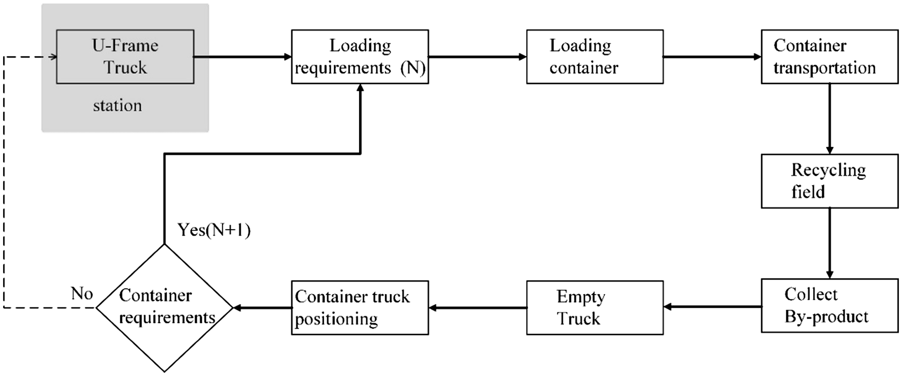
Transport flowchart of steel mill by-product.

Moreover, the case-by-case transportation of by-products is carried out in the manner of zoning. Based on the zoning operation, the study investigated the minimum total transportation time by the use of genetic algorithm and minimized the difference of transport time between different districts, in order to avoid management problems caused by uneven work and rest periods. The transportation time of each subarea is optimized in terms of route requirements among the various needs to be explored in consideration of vehicle routing issues, as shown in Figure 4(a) where the square pattern shows the station and the circle pattern indicates the demand point of container requirements. However, the transportation time increased by the field back and forth travel, as shown in Figure 4(b) where the recycling field and the container transportation route should also be considered. That is seldom mentioned in the related literature on this kind of problem. Hence, this study will explore the optimal weight distribution mode in order to effectively find the best transportation mode.

Figure 4.

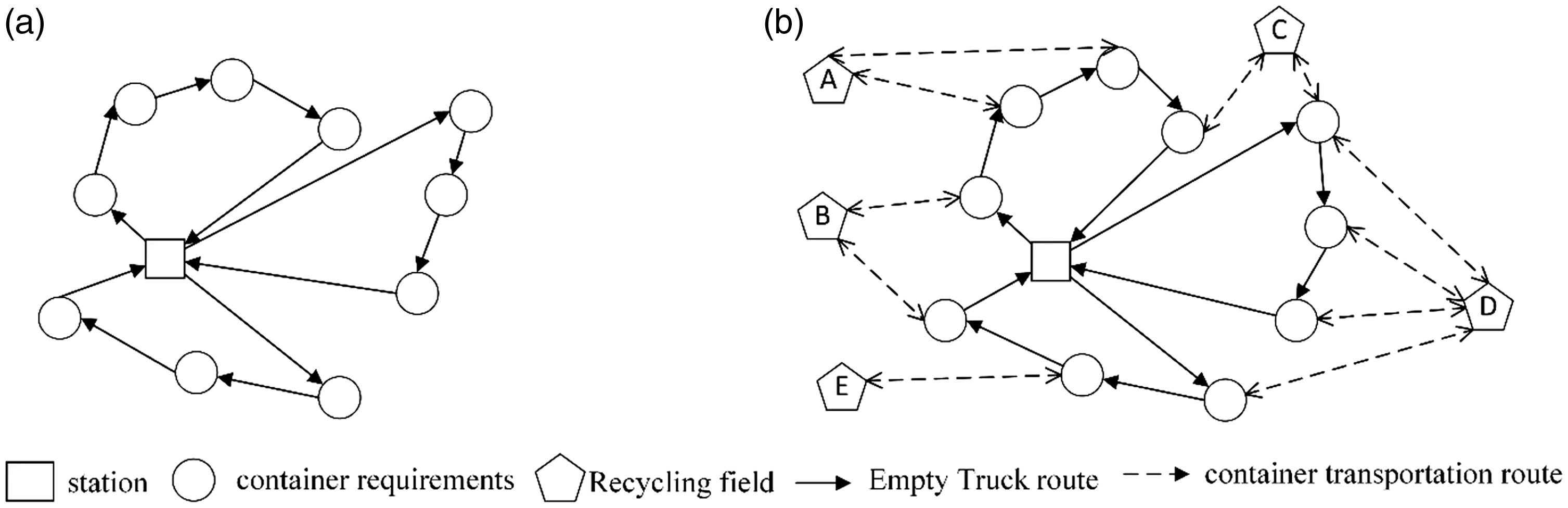
Comparisons between: (a) a conventional VRP route and (b) the case study’s by-product route.

The case study’s by-product transport model for the company’s factory is shown in Figure 5. Each loading cabinet has a designated recycling yard due to the different types of materials loaded, so that by-products can be handled effectively. The positions cannot be changed arbitrarily. For example, the loading demand point {1} can only dump the materials to the designated recycling market {D}, and the transportation routes with the same trip back and forth must return to the original position after dumping; {5} can only be dumped into the designated recycling market {B}, the same transportation path back and forth must be followed, and after the dumping, the vehicles must return to the original position, in the absence of loading demand cancelation under the transport path: {0} → {1-D-1} → {2-C-2} → {3-A-3} → {4-B-4} → {5-B-5} → {0}. The transport path under demand cancelation is: {0} → {1-D-1} → {2-C-2} → {3} → {4-B-4} → {5-B-5} → {0}, to indicate whether there is a need to cancel the loading requirements. The vehicles are required to arrive at each loading point; only the shipping route between loading {3} and recycling {A} is canceled because the by-product output depends on the production process. At this stage, vehicles approach the loading position to check to see if there is any requirement for carriage. If it is necessary to transport the load to the designated recycling yard, the container is dumped back in its original location and then moves to the next loading position; if no load is required it goes straight to the next loading location and returns to the parking lot after completing all the shipping tasks {0}.

Figure 5.

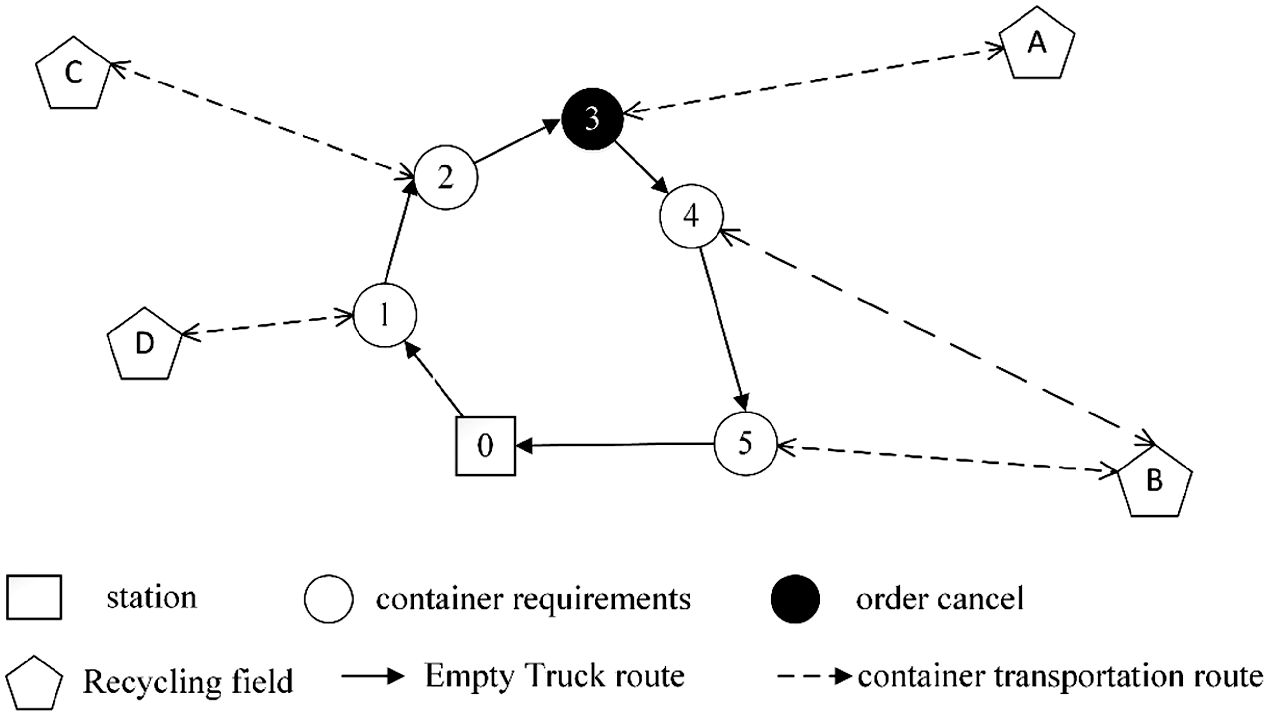
By-product transportation route.

Shipments of by-products are not affected by the temporary cancelation of the demand and are still visiting each loading location on the original planned route, which can be categorized as Fixed Routes described in the study by Sungur¹³ with poor transport efficiency; however, the analysis of the geographical distribution of the plant site and the loading demand point are limited, covering a total area of only about 3 × 3 km. In addition to the main road, most roads are designed by Dead End. Loading cabinets and vehicles installed on both sides of the same Dead End or in the workshop enter the road to learn the filling status of loading by-products, as shown in the deadline of the Dead End Road in Figure 6. When the demand of loading {3} is canceled, the total driving distance will increase only slightly; the sections are not counted and can also be classified as semi-fixed routes.¹³

Figure 6.

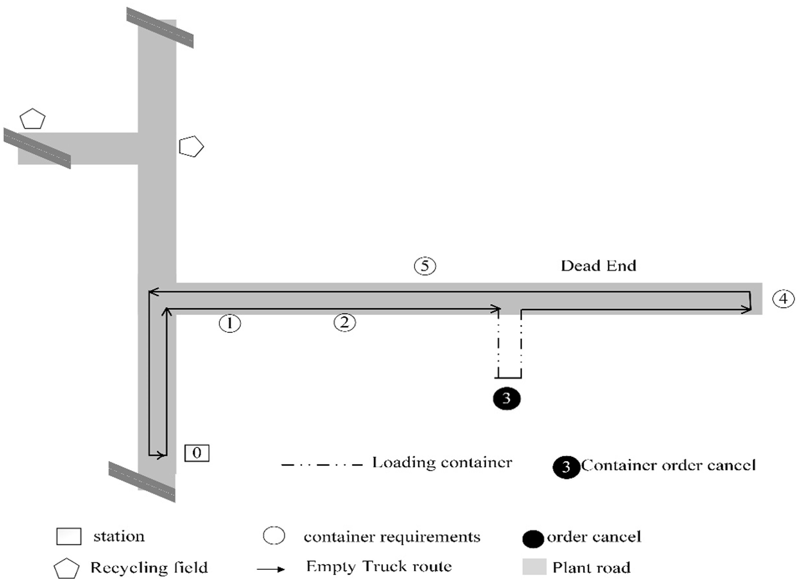
Dead End of container transportation route simulation.

With the company’s plant environment configuration, manpower and funding in a temporary cancelation of the construction of the system can employ a re-planned path to the current mode of operation. The reduction of the total driving distance is limited, and the economic benefits are clearly not good. In contrast with the problem of staff scheduling and management, it is advantageous to maintain the transportation by fixed or semi-fixed route. However, it is quite important to partition the loading cabinet. This study will take the first grouping path planning strategy. The algorithm first explores the case company partitioning mode of operation and then derives the best route for each partition.

In summary, this study uses a fixed path approach to explore the optimal partition combination; the minimum total transit time can be obtained, as well as minimizing the difference between the operating hours of vehicles in each partition. The main influence variables of each responsible partitioning operation time of the case company and the transportation time of each responsible partition are as follows:

Travel time between loading points in each sub-district, as well as driving time between parking lots and loading cabinets

The loading requirements of the sub-district loading point frequency. The theoretical expresses of the model are shown in following:

Z t_{j} = \sum_{i = 1}^{n} C w_{i} + \sum_{i = 0}^{n} d_{i}

(1)

C w_{i} = C f_{i} \times C t_{i}

(2)

where

Z t_{j}

The jth partition of the total transport time.

C w_{i}

Any load weight for the carrier frequency and loading transport operation time product.

d_{i}

The empty travel time from Loading i to Loading j + 1 includes the travel time from the parking lot to the loading demand point and the travel time to the parking lot at the last loading demand point.

C f_{i}

Loading carrier frequency

C t_{i}

Loading transport time: for loading to the designated recycling field transport operations back and forth, including loading and unloading time, loading dumping time, and loading positioning time

n

Responsible for the number of cabinet demand points partition

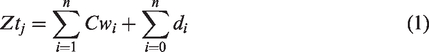
Equation (1) shows the total transport time of any responsibility zone, which is the empty travel time of all the load points in the responsibility zone plus the weight of all load point requirements, that is, the total transport time of each responsible zone except that when influenced by the demand of loading, it is also affected by the weight of each loading. Equation (2) shows the weight of each load, which is the product of the load carrier frequency and load transport time. The loading frequency is the transport demand during the company’s production cycle; it can be converted into the possible number of load trips per class per day to assess the differences in the total transport time for each responsible partition during the production cycle; in practice, the loading frequency may be different for each class in practice, but the difference in transport time for each responsible partition can still be controlled during the production cycle, within reasonable limits.

Proposed DLGA

In this section, the DLGA is employed. We assign different loading requirements for every cargo partition to minimize working time and achieve the best fitting transportation times. Such a time schedule can be calculated by checkerboard pattern foam chromosomes under the premise of fixed chromosomes length; it then deals with the coding approach for piggyback factory transportation in this proposed approach. All these encoding, initial population, adaptation function, selection and reproduction, mating, mutation, termination condition, and other stages of calculation process will be investigated.

DLGA based on checkerboard chromosome with foam gene

To obtain minimum piggyback factory transportation in the case of partition mode operation in which the by-product logistics are loaded and that will belong to the multi-objective vehicle routing optimization problem, we will resolve the vehicles schedule between whole area transporting routes and partition subarea arrangement planning first; then we can optimize the partition subarea loading routes. The design flowchart of DLGA is illustrated in Figure 7 and described as follows:

The first layer algorithm resolves the whole area transporting routes under a suitable partition subarea arrangement. Each uploaded point of the piggyback operation for suitable transportation will be encoded as chromosome representation; it will be substituted into the fitness function to evaluate the standard deviation time between the whole area transporting routes and the accumulated subarea loading routes. The program will optimize the fitness condition via replication, mating and mutation to obtain the suitable parameters as the initial conditions of the program solution.

The second layer algorithm concerns the partition subarea loading routes. It deals with the planning arrangement of the partition subarea; meanwhile, it optimizes the minimum time schedule for all the partition subarea loading routes accumulated.

Figure 7.

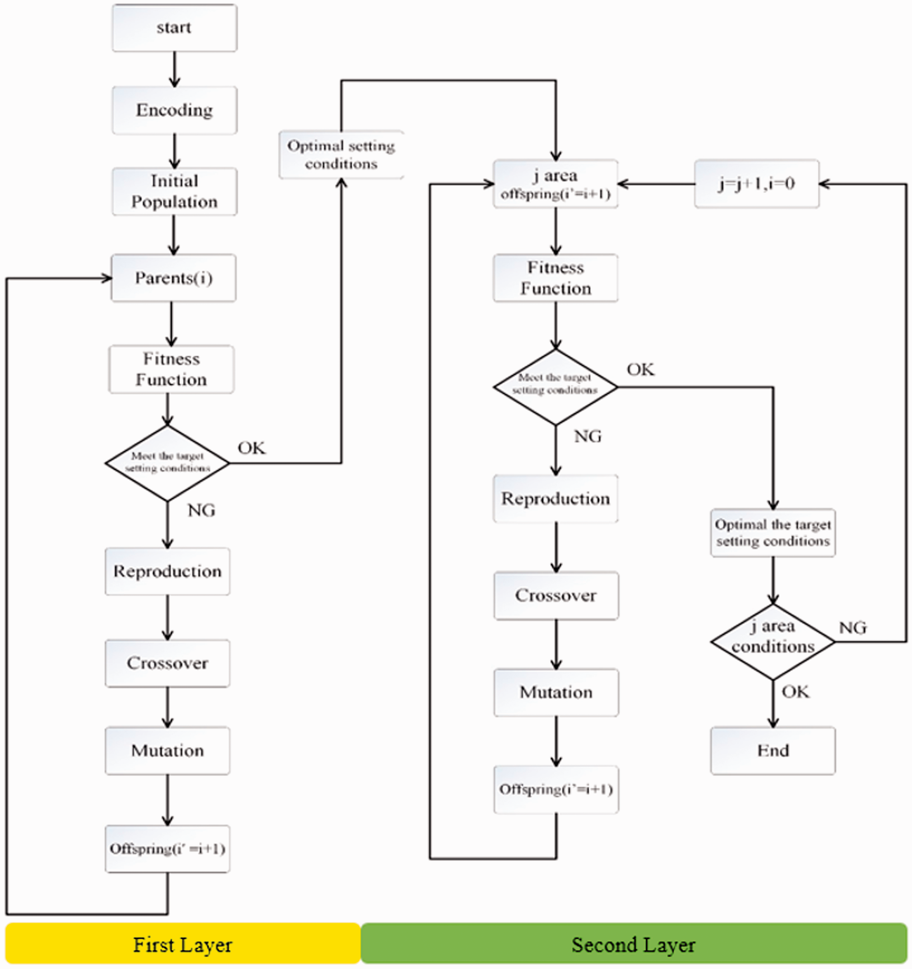
Flowchart of the double-layer genetic algorithm.

We chose transportation time as the objective function in order to obtain the optimized time difference among discrete subarea transportations. The distances and weights among different loading locations are not the same. Under the goal of achieving equal transporting time for different subarea loading, the distribution numbers of uploading locations for every subarea must be adjusted in accordance with the example. Feasible chromosome coding will be considered in these examples for efficiency improvement. The concept is that the chromosomes of a genetic algorithm will be fixed in length and will not evolve generation by generation in the traditional optimized design.¹⁴ However, its defect will appear in a complicated example as the optimal fit value could be limited by the chromosome length of the original set conditions. A shorter chromosome length will not obtain an optimal solution owing to less diversity of selective arrangement. Foam chromosomes can be embedded with a checkerboard pattern into a genetic algorithm to resolve the subarea partitions transport operations problem because of proper diversity of arrangement with fixed length chromosomes.

Each different subarea partition will be represented with checkerboard foam chromosome C_i and each checkerboard pattern set default will have the same locus. The numbers of genetic loci correspond to the numbers of uploading locations for every subarea partition. If the total length of chromosomes is designated as L for all subarea partition numbers up to z, as equation (3) shows, all numbers of checkerboard chromosome C_i are multiplied by the number n of checkerboard loci:

L = \sum_{i = 1}^{z} C_{i} \times n

(3)

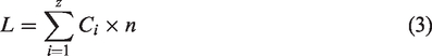
Assume that the whole uploading locations N in this factory can be equally divided into numbers z of a subarea partition; the total loci numbers of individual checkerboard chromosome will then be n = N/z, as we round up n to be an integer. Under the actual subarea partitioned circumstance the numbers of uploading locations assigned to each partition will not be equal; thus, when we equally assign the numbers of chromosome loci in one checkerboard, it will appear that this approach results in a finite solution owing to less diversity in the selective arrangement. Assume that the loci numbers of chromosome was given with n in advance; we must add additional loci numbers with m appropriately in order to obtain the optimal arrangement of partition operations. The total loci numbers n of single checkerboard chromosome can be expressed as:

n = (N / z) + m

(4)

As described above, the total numbers n of loci in the whole chromosome lengths L had additional loci arrangement numbers with m such that the genes d_i of the whole uploading location could not be fulfilled with every locus after integer coding. The remaining vacated sites of loci must be filled with a number 0; that is what we call foam gene to act as the function of foam sponge filled in empty gene locations of checkerboard chromosomes. During the process of solving the optimal arrangement for each subarea partition, we can increase the number 0’s of foam genes to fill vacated sites of loci when the genes numbered d_i of whole uploading location were assigned less than were required in a single checkerboard chromosome. On the other hand, we can reduce the number 0’s of foam genes to make a concession in occupying vacated sites of loci when the genes numbered d_i of the whole uploading location were assigned more than were required in a single checkerboard chromosome. That is a suitable approach to keep the total length of chromosome fixed for solving the optimal arrangement of the subarea transporting operation; the uploading location could even be arbitrarily adjusted. The arranged structure of the checkerboard pattern Foam Chromosome is shown as Figure 8. The loci numbers m of foam genes should be properly adjusted incrementally or excessive foam genes will result in too long chromosome length and problem solving time. But the possibility of optimal solution will still be confined due to fewer foam genes being provided.

Figure 8.

Checkerboard chromosome with foamed gene.

Figure 9.

Asexual Random Reverse Crossover.

Optimal design process of DLGA

Step (1): Variable encoding and initial chromosome population

In the first layer algorithm, we make every uploading location an integer encoding so the second layer algorithm encoding would not be needed. Then, it will randomly generate numbers n of the initial chromosome populations.

Step (2): Fitness function

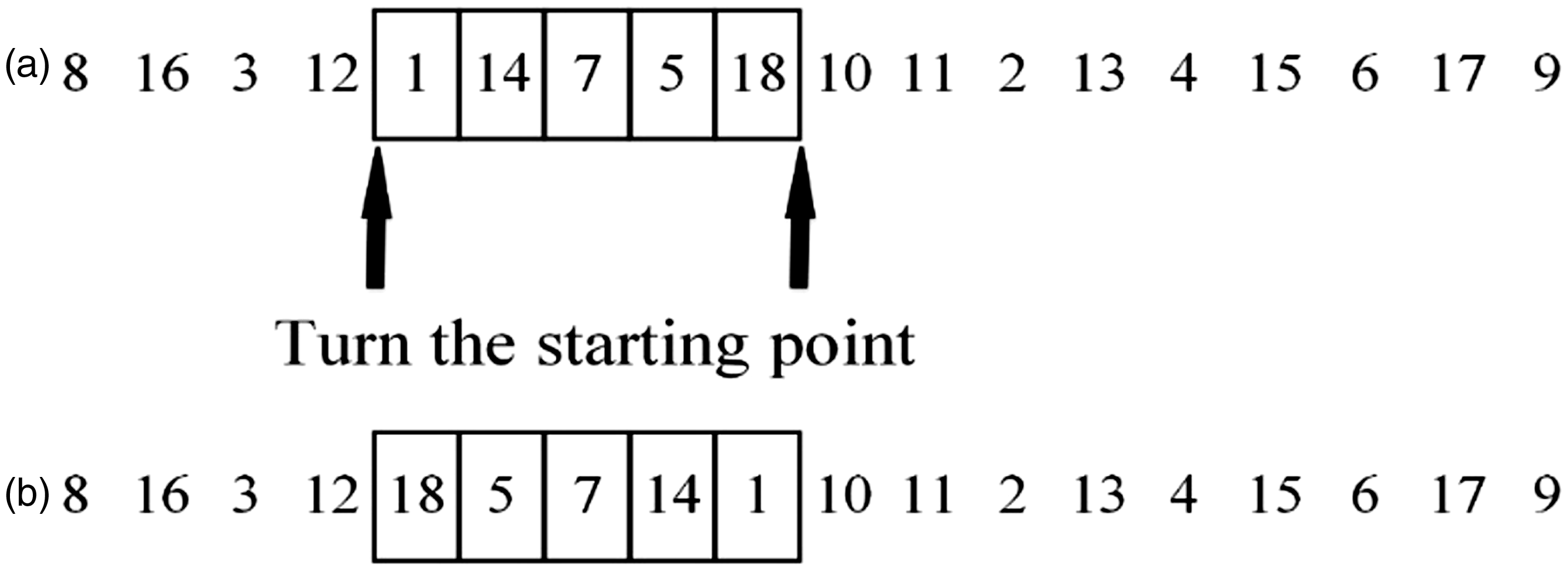
Fitness function is mainly used to estimate the extent to which chromosomes adapt to the environment; better ability will be represented as greater area occupied on the roulette; the better opportunity of being selected can then evolve and those good genes with a competitive advantage for the next generation retained. That will gradually approach the best fitting solution. In this study, we perform the DLGA in that the first layer algorithm evaluates the fitness function for each subarea transportation time as in equation (1); the standard deviation of transportation time in each subarea is shown as equation (5)

σ = \sqrt{\frac{Σ {(Z t_{j} - \bar{Z} t)}^{2}}{Z}}

(5)

and the total transportation time will be as expressed in equation (6)

\sum_{j = 1}^{Z} Z t_{j}

(6)

The second layer algorithm performs the optimization for the standard deviation of each subarea transportation time. In this layer algorithm, the fitness function for each subarea transportation time is still as expressed in equation (1) and the standard deviation of transportation time in each subarea as in equation (5).

Step (3): Selection and reproduction

We use the method of roulette wheel selection to stochastically create a random number with the decimal value between 0 and 1, with the value falling within the accumulation interval of the roulette wheel; the chromosome represented by this interval will be selected for reproduction. Both stages of two layer algorithm use the same selection and reproduction methods.

Step (4): Crossover

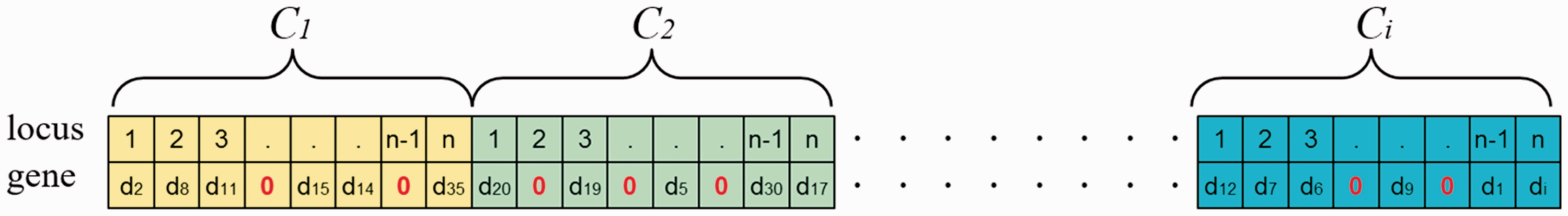
Traditional crossover mechanism picks two chromosomes and exchanges each side genes of a selected crossover site for each other, in order to retain optimal parent genes for the next generation and produce optimal genes combination for suitable chromosomes. With the collocation of checkerboard foam chromosomes in our study, we selected asexual random reverse crossover to operate in both stages of the DLGA. Asexual random reverse crossover differs from the traditional crossover operation because the crossover site selected and genes exchanged operate on the same chromosomes. The operation steps will be performed as follows:

The first is stochastic creation of two transposed sites on the selected chromosome for crossover operation, as shown in Figure 9(a).

The second is genes inverse transposed; we reverse the genes arrangement between two transposed sites that are selected in advance to synthesize a new chromosome, as shown in Figure 9(b).

Step (5): Mutation

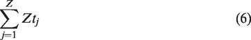
The mutation operation performs the mechanism to jump out of the current searching interval during the process of algorithm and avoid falling into local solution interval in order to obtain the global optimal approximate solution. In this study, the same uniform random crossover mutation is adopted for both stages of the DLGA. Each gene in the chromosome has its own probability value P which is generated stochastically. When the probability value P is less than a default value of mutation probability, this gene site will be selected as the mutation point. For the selected mutation point gene, an exchangeable mutation gene locus with value Q will be generated randomly (loci sorting from left to right) in order to exchange both genes. Figure 10 illustrates this procedure for uniform random mutation and is described as follows:

Figure 10.

Uniformly Random for Swap Mutation.

Each 10 genes in the chromosome will separately randomly generate a probability value P. Among them, the probability values of individual genes “3,” “7,” and “9” are all less than the default value of the mutation probability. These three genes will be chosen as the mutation points.

For the chosen gene sites “3,” “7,” and “9” as the mutation loci, the probability accompanying these loci will again be separately randomly generated as value Qs, such that the probability of gene “3” could be randomly generated as Q=5; it means that gene “3” will be interchanged with the fifth gene “1” of the chromosome sequence from left to right. The similar probability is that gene “7” could be randomly generated as value Q=2: represented as gene “7” interchanged with the second gene “6” of the chromosome sequence. Also the probability of gene “9” could be randomly generated as value Q=6 and then represented as gene “9” interchanged with the sixth gene “4” of the same chromosome sequence.

The mutation process is completed after the two genes are exchanged. There no restrictions on gene interchange, which can be interchanged with itself or with the chosen mutation locus of the gene.

Step (6): Termination condition

It will be terminated when default fitness value, the maximum number of iterations or fitness value stagnant algebra will be reached.

Optimal analysis and result discussion

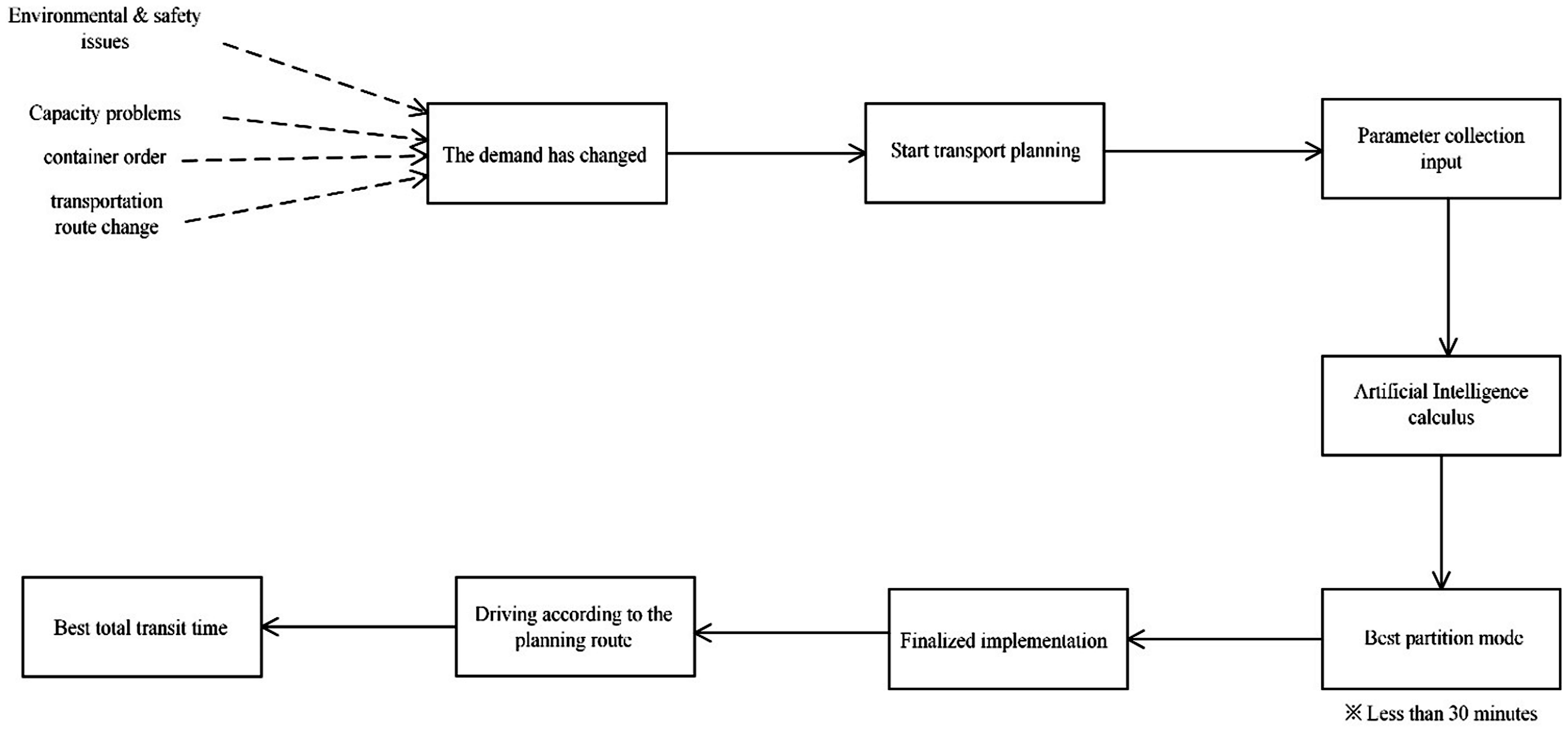
This research case is an integrated steel mill, which uses U-frame carriers with multiple cabinets to efficiently classify and upload different classifications of by-products. But the fuel consumption of U-frame carriers is higher than ordinary container vehicles, so that appropriate transportation planning will be very important in times of economic depression. According to customary practice, the transportation planning will highly depend on experience of relevant experts and will take much mental and physical effort to obtain results that may not be optimal. Artificial intelligence (AI) would be the best approach to overcome the barriers for transportation planning time and optimal subarea partition operation for minimum transportation time.

We consider the first shift schedule for the subarea transportation operation as an example. In order to obtain minimum transportation time and optimal partition operation that we discuss the constraint conditions as follows:

Single parking facilities whose locations are known.

There are eight recycle processing farms which are known; the same kinds of by-product from different production lines are loaded within the same cabinet in each recycle location.

There are 116 uploading locations at known positions. Each cabinet can be loaded with a single kind of by-product only; there can’t be mixed loading. Each kind of recycled by-product must be dumped into its designated recycling farm.

Empty vehicle transportation time: In one trip time, the time spent for driving path between two cabinet uploading location as well as driving path between parking lot and uploading each location are specified.

Loaded vehicle transportation time: Regarding the cabinet transport on load, we can express the transportation time with load as [loading and unloading recycling time] + [load carrying time] + [loading and unloading positioning time] + [dumping by-product time]. Each vehicle’s loading time is different either owing to the environment’s effect on loading operation or to the distance varying between different loading sites and recycling farms.

Each cabinet corresponds to one vehicle per shift. When the vehicle reaches the uploading location, it will be transported to the specified recycling site for dumping if it is loaded; otherwise, this vehicle will move to the next uploading site for no shipping requirement or transportation completion.

Cabinet loading frequency is the shipping amount of times during the production cycle. It means the total shipping amount per month is equivalent to the shipping rate in one day.

Loading for shipment will be whole vehicle type; it means the vehicle capacity equals shipping capacity and there are only two options with “on load” or “no load” operation for shipments.

The U-frame vehicle drives the same round-trip path between the uploading site and recycle farm. The uploading locations cannot be changed arbitrarily. We assume that the transportation distance (operation time) between uploading location and recycle farm will be constant.

In each shift, a task vehicle departs from the parking lot. When it has completed the shipping task within each area of responsibility, it will then return to the original parking lot.

Each cabinet can only belong to one area of responsibility. Under normal production conditions, the factory area can be divided into six subareas of uploading locations on which a single vehicle operates and over which it cannot cross.

One driver operates one single type piggyback vehicle with one cabinet per trip.

Suppose that the average driving velocity is moving at 15 km/h: Velocity limit in the factory is 30 km/h, but on part of intersection limitation of velocity will be 20 km/h and 15 km/h for level crossing, and 10 km/h for workshop aisle. Together with delayed time by traffic light, the average speed of the vehicle will be 15 km/h.

Each vehicle operates 8 h per shift, in addition to driving hazard prediction for 0.5 h, vehicle inspection before driving for 0.5 h, vehicle refueling for 0.5 h, lunch and rest for 1 h and cleaning of the vehicle after finishing work for 0.5 h, the real time for a driver to operate in duty should be less than or equal to 5 h.

Comparison for partition planning

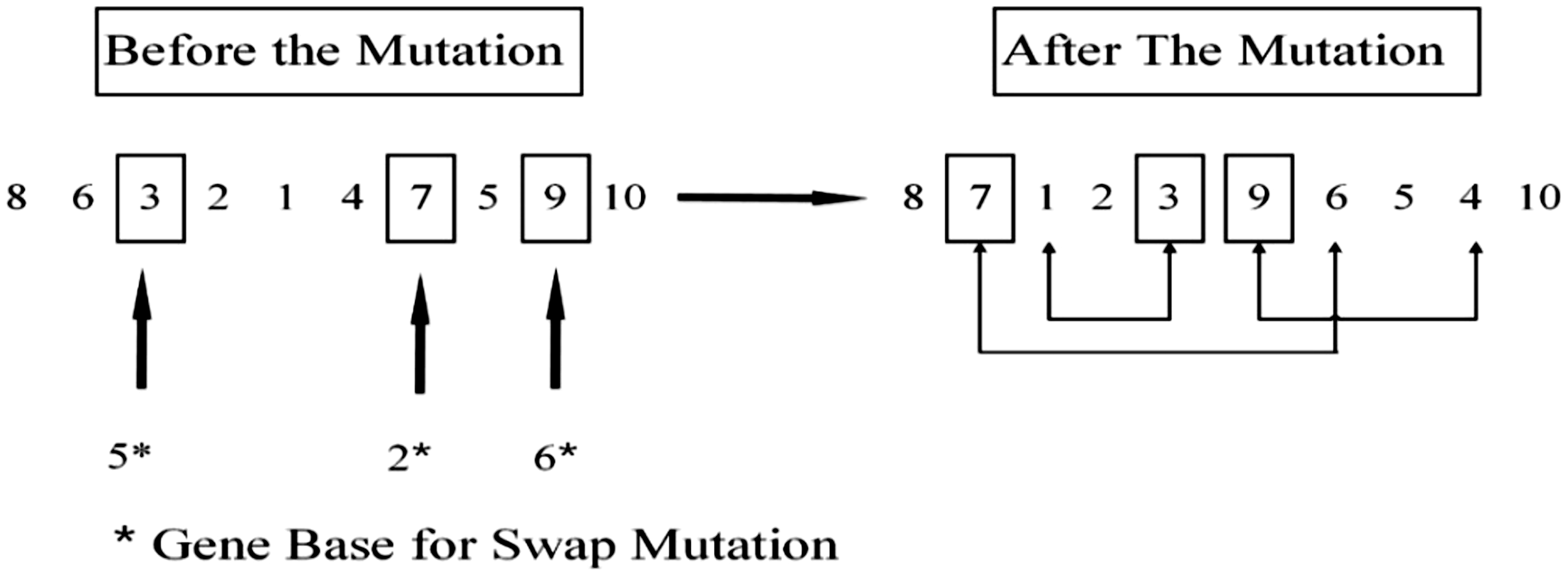
In order to clearly compare the differences between artificial partition planning and DLGA partition planning, the following section shows a flow chart for these two partitions’ planning and describes them. The work time for artificial planning will also be evaluated and analyzed.

The partition planning operation should be restarted when there is a noticeable change in the uploading requirement. The artificial operation relies on experience and refers to basic criteria at the current stage. The empirical value is essential to influence the partition planning and planning time. In addition, because artificial planning also involves personal preferences and abilities, the results of the plan should be discussed among all drivers for implementation after consensus has been reached. Whether the result is attributed to an optimized partitioning job process is not validated. The artificial planning job flow chart is designed in Figure 11.

Figure 11.

Manual planning operations flow chart.

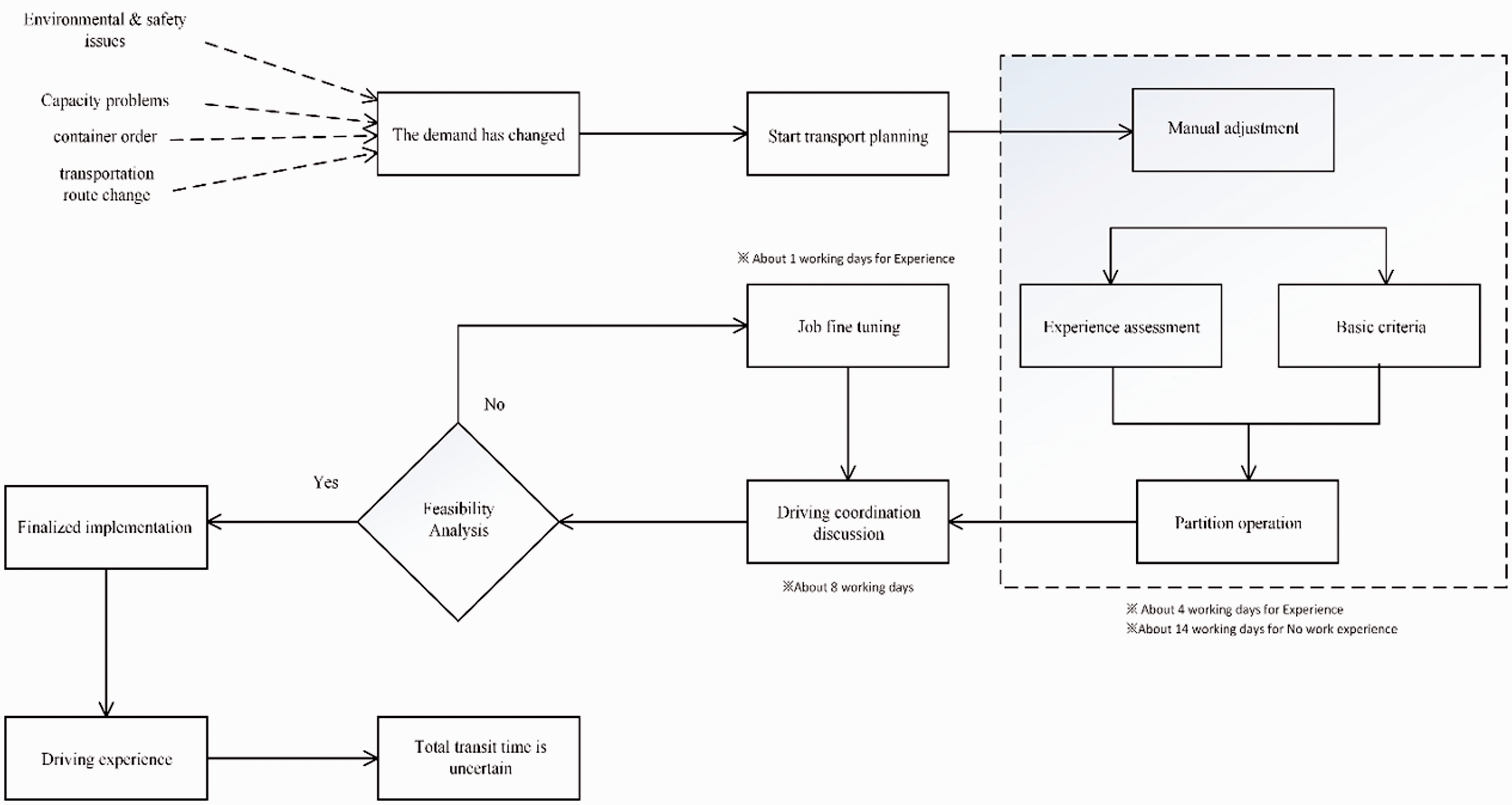
At present, the partition planning of this factory relies on artificial work. The time matrices expressions for uploading-recycling the farm-parking lot have not yet been established. Practitioners with and without experience will have a significant impact on the overall job planning. In terms of more than 100 cabinets for scheduling, we must control the cabinets uploading locations, data collection for shipping requirement and partition planning. After a discussion among all the drivers, the partition planning job will be fine-tuned so that this plan draft can be finalized and implemented. Evaluation is time consuming for the first draft; while a practitioner without experience takes about 14 working days, a practitioner with experience takes only 4 working days. The main difference between these practitioners is the understanding of the uploading location arrangement. The time evaluation for the draft of artificial partition planning is listed in Table 1.

Table 1.

Time evaluation draft for the artificial partition planning.

	Know the location of the scene loading	Carrier demand data collection	Partition planning homework	Fine-tuning partition planning jobs	Total working days
Without experience	7 days	2 days	5 days	1 days	15 days
With Experience	1.5 days	1 days	2 days	0.5 days	5 days

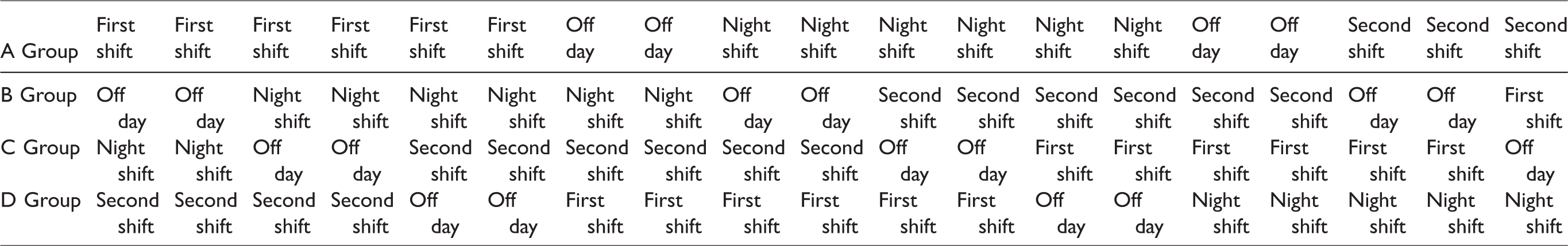
There are four transportation sections for by-product shipping in this factory. The work schedule is divided into three shifts 24 h a day (early, middle, and late). Each shift schedules one transportation section to attend, while another is scheduled to take a break. All transport sections work for six days and rest for 2 s on early shift. The other schedules still work for six days and rest for the middle and late shifts. The implemented shift schedule is presented in Table 2.

Table 2.

Shift schedule to be implemented.

A Group	Firstshift	Firstshift	Firstshift	Firstshift	Firstshift	Firstshift	Offday	Offday	Nightshift	Nightshift	Nightshift	Nightshift	Nightshift	Nightshift	Offday	Offday	Secondshift	Secondshift	Secondshift
B Group	Offday	Offday	Nightshift	Nightshift	Nightshift	Nightshift	Nightshift	Nightshift	Offday	Offday	Secondshift	Secondshift	Secondshift	Secondshift	Secondshift	Secondshift	Offday	Offday	Firstshift
C Group	Nightshift	Nightshift	Offday	Offday	Secondshift	Secondshift	Secondshift	Secondshift	Secondshift	Secondshift	Offday	Offday	Firstshift	Firstshift	Firstshift	Firstshift	Firstshift	Firstshift	Offday
D Group	Secondshift	Secondshift	Secondshift	Secondshift	Offday	Offday	Firstshift	Firstshift	Firstshift	Firstshift	Firstshift	Firstshift	Offday	Offday	Nightshift	Nightshift	Nightshift	Nightshift	Nightshift

The work flow for studying partition planning with DLGA is shown in Figure 12. It is necessary to prepare in advance the locations for uploading and to establish time matrices for cabinet-recycling field-parking lot round trips. Care must be taken as the accuracy of data collection could directly affect the output of the results. The advantage of a DLGA algorithm is that the global optimal solution can be obtained in a reasonable amount of time, and the optimal transport schedule for each partition can be found, as well as the reasonable transportation time difference between different zones. There are apparent data on corroboration for calculation results; it can effectively shorten the time spent for communication and coordination, thereby improving the overall efficiency in planning the work.

Figure 12.

Planning work flowchart based on DLGA.

Figure 13.

Checkerboard chromosome with Foamed gene of 6 partition.

Workflow comparison between Manual partition planning and DLGA partition planning

Artificial partition planning does not establish time matrices for cabinet uploading-recycling field-parking lot round trips that are not a standardized operation but are all done according to staff experience and memory. With the time matrices established in this study, the partition planning operation can be standardized with the help of DLGA, and the current results of artificial partition planning can also be verified.

Artificial partition planning is a lengthy process. Any planner without experience needs to control and understand the situation on the site before planning an optimal partitioning operation, while an experienced planner can shorten time effectively. Whether or not there is experience, it will take 13 to 23 working days, and the experience of planners is the key factor affecting the results. To implement the partition planning with DLGA, it is necessary to collect the relevant parameters about uploading locations together with DLGA computing time so that the overall planning work can be completed within half an hour. The accuracy of the parameters collected will be another key factor influencing the planning results.

Artificial partition planning does not schedule the transportation for every uploading location; it depends on the experience of the drivers themselves. DLGA is used for partition planning; in addition to obtaining the optimal transportation time in the whole factory, the optimal shipping schedule for each partition can be planned immediately. It won’t take a long time for trial and error to increase transportation costs.

Vehicle driving is an NP-Hard problem, so the best solution cannot be obtained in reasonable time. In addition to a lot of time being required for planning by the artificial partitioning of administrative staff, no data can be verified as optimal mode, so that it is necessary to discuss with drivers to obtain better results. The process is laborious and time-consuming mixed with excessive human factors, so that it cannot become a standardized operation. The improper handling in this process could easily influence the organizational unity. Partition planning aided by AI can obtain the optimal solution of the whole factory in a reasonable time and standardize this operation, effectively improving the efficiency of the partition planning.

Results of six companies in case study

This section compares the results of DLGA solutoins with the six-zone operations of the current company. The following subsection solves the current situation of manual zone partitioning with time matrix, which is followed by a subsection that describes the related parameters of genetic algorithm and the solution result; and the final subsection offers a comparison between manual partitioning and DLGA solution, draws the artificial partition of the district and the region transport route map, and DLGA district and the region transport route map, to compare the differences between the two.

Analysis of the status of artificial zoning

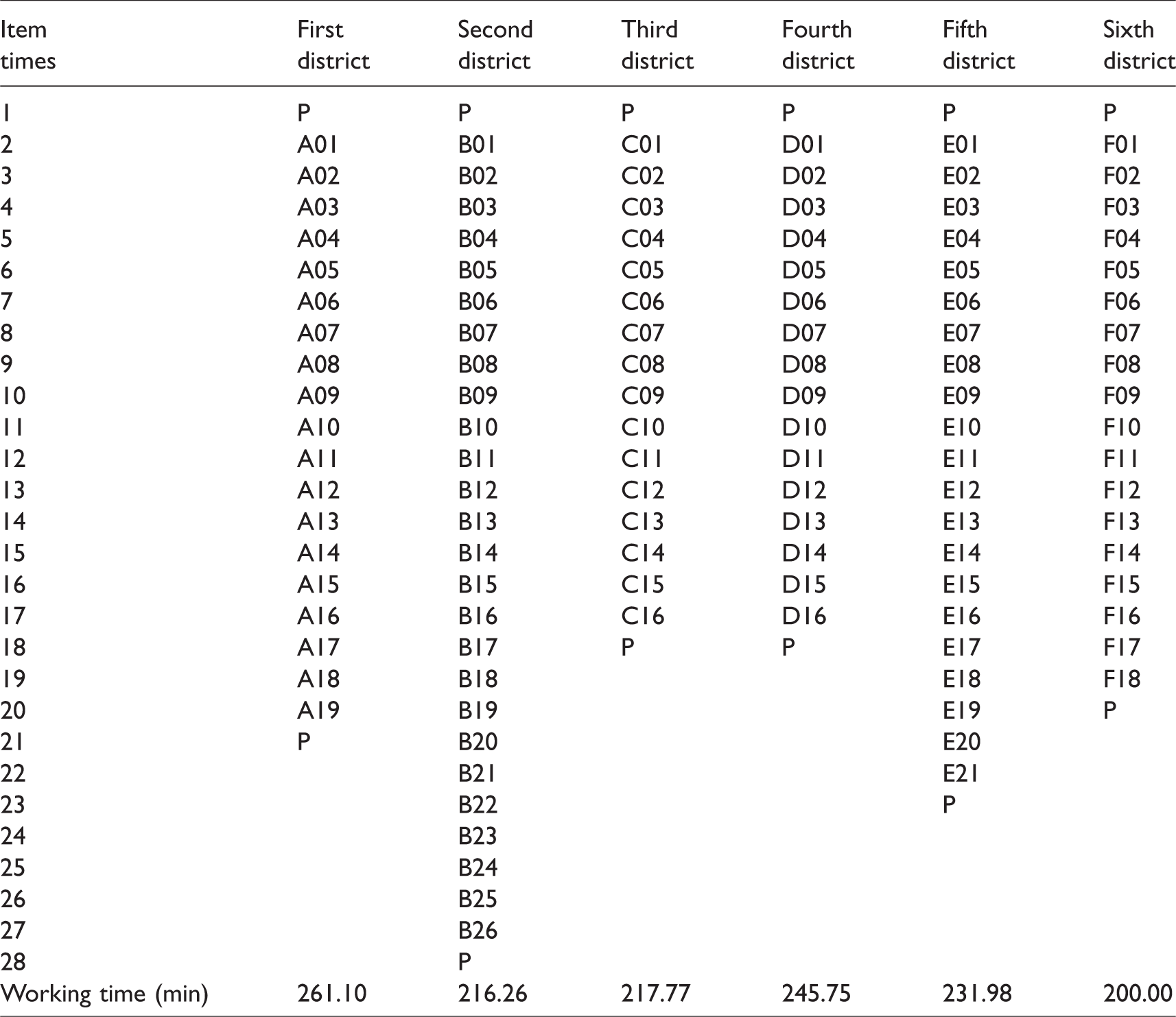
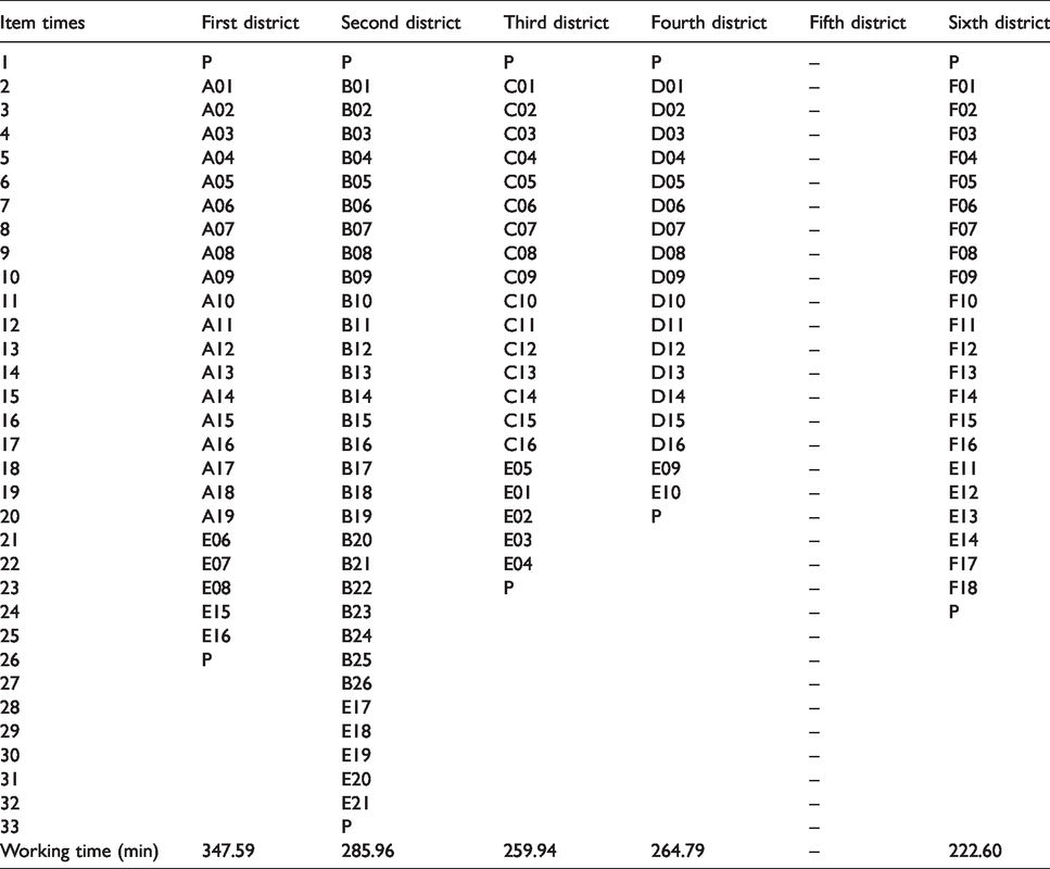
The case study was based on Table 3 for the manual division of the six divisional early-morning schedules. The divisional assignment was planned by experienced staff and the load-carrying schedule for loading points in each divisional area was also an experienced driver's plan The transportation route taking Zone 1 as an example is P (parking lot) → A01 → A02 → A03 → … A18 → A19 → P (parking lot), and the collection and recovery yard established by this research, with the parking lot time matrix, calculating the transportation time of each partition including the loading transport weight, Zone 1: 261.10 min, Zone 2: 216.26 min, Zone 3: 217.77 min, Zone 4: 245.75 min, Zone 5: 231.98 min, 6th zone: 200.00, the maximum zone transportation time is 261.10 min, the minimum zone transportation time is 200.00 min, the standard deviation of transportation time of each zone is 22.13 min; the total transportation time of the whole zone is 1372.85 min.

Table 3.

Manual planning six districts first shift schedule.

Itemtimes	First district	Second district	Third district	Fourth district	Fifth district	Sixth district
1	P	P	P	P	P	P
2	A01	B01	C01	D01	E01	F01
3	A02	B02	C02	D02	E02	F02
4	A03	B03	C03	D03	E03	F03
5	A04	B04	C04	D04	E04	F04
6	A05	B05	C05	D05	E05	F05
7	A06	B06	C06	D06	E06	F06
8	A07	B07	C07	D07	E07	F07
9	A08	B08	C08	D08	E08	F08
10	A09	B09	C09	D09	E09	F09
11	A10	B10	C10	D10	E10	F10
12	A11	B11	C11	D11	E11	F11
13	A12	B12	C12	D12	E12	F12
14	A13	B13	C13	D13	E13	F13
15	A14	B14	C14	D14	E14	F14
16	A15	B15	C15	D15	E15	F15
17	A16	B16	C16	D16	E16	F16
18	A17	B17	P	P	E17	F17
19	A18	B18			E18	F18
20	A19	B19			E19	P
21	P	B20			E20
22		B21			E21
23		B22			P
24		B23
25		B24
26		B25
27		B26
28		P
Working time (min)	261.10	216.26	217.77	245.75	231.98	200.00

DLGA solution

Taking the load-recovery field, the parking lot time matrix and the loading transport weight, we imported the double-layer gene algorithm constructed in this study. The relevant parameters of the six zones were set as follows:

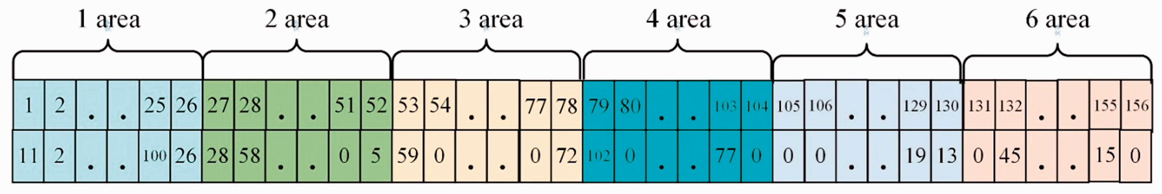
Integer encoding: The first layer of gene calculus randomly generated 2000 initial chromosome populations; the second layer of gene calculus randomly generated 200 initial chromosome populations.

The first layer of gene calculus, with checkerboard foam gene chromosomes, equipped with six chessboards, each board’s configuration 26 base, and foam gene 40, is shown in Figure 13 hexagonal checkerboard foam gene chromosome structure; the second layer gene calculus is optimized by the path of each partition board.

Adaptation function: the first layer of gene function evaluation of the adaptation function of the total transport time zone, transport time of each partition and transport time standard deviation of each partition; the second layer of gene function evaluation of the adaptation function is the partition transport time and the partition transport standard deviation of time.

Using the roulette method, the copy rate was chosen to be 0.85, and the first and second floor genes were all alike.

Asexual random mating, mating rate of 1.0: the first and second genetic algorithms are the same.

A uniform random crossover mutation, mutation rate of 0.3; the first and second genetic algorithms are the same.

Terminate conditions: reach pre-set fitness or iterate 20 million times.

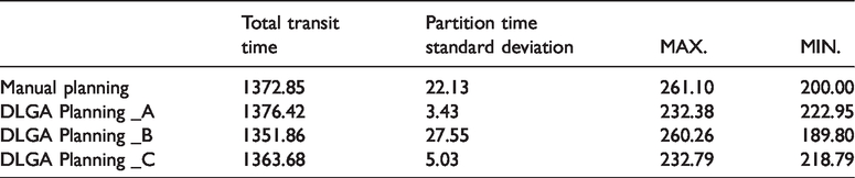
According to the case study, we calculated the three solutions of A, B and C, respectively, as shown in Table 4. The other four quadrants were drawn from the results of artificial partitioning: X coordinates for the total transit time and Y coordinates for the standard deviation of transport time zone were marked as DLGA of each solution to assess the merits of the DLGA solution, as shown in Figure 14, DLGA Planning Pareto Solution.

Figure 14.

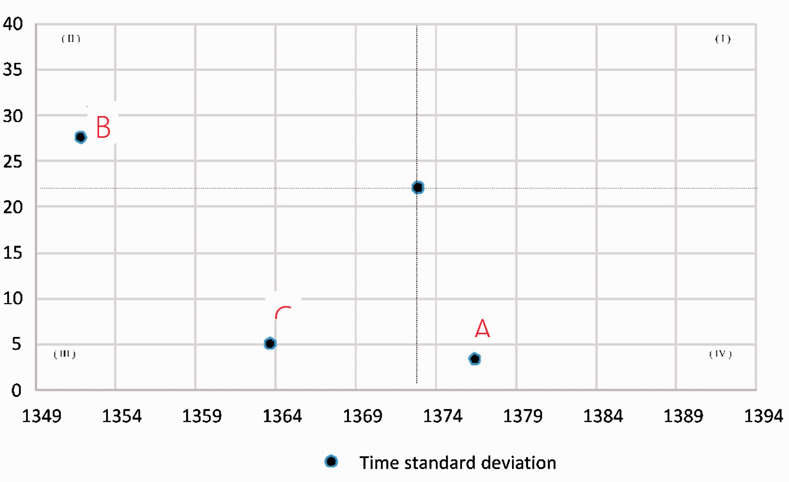
DLGA Planning Pareto Analytic Solution.

Figure 15.

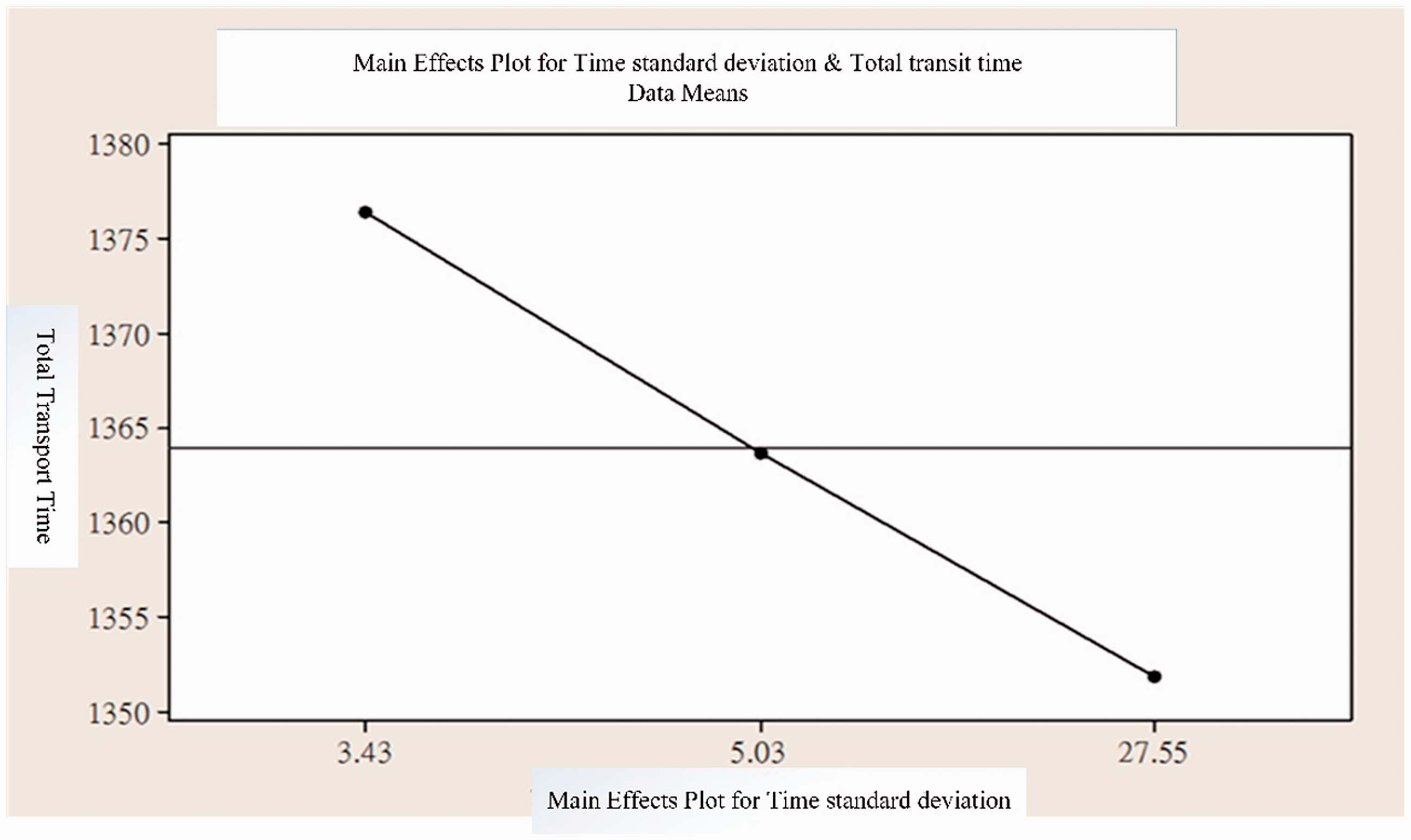
Main effects plot for time standard deviation and total transit time data means.

Figure 16.

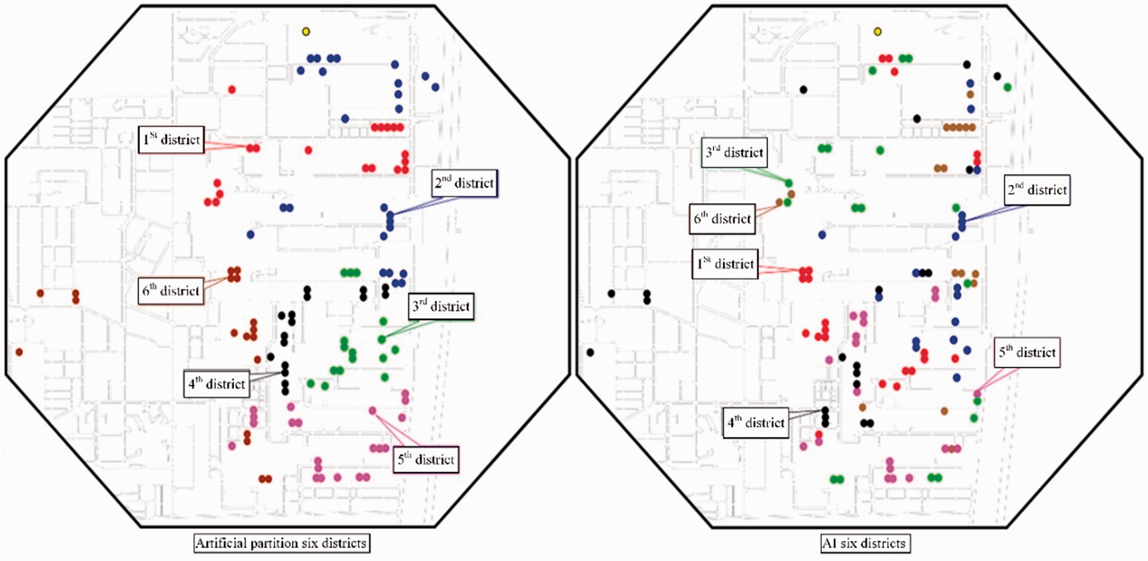
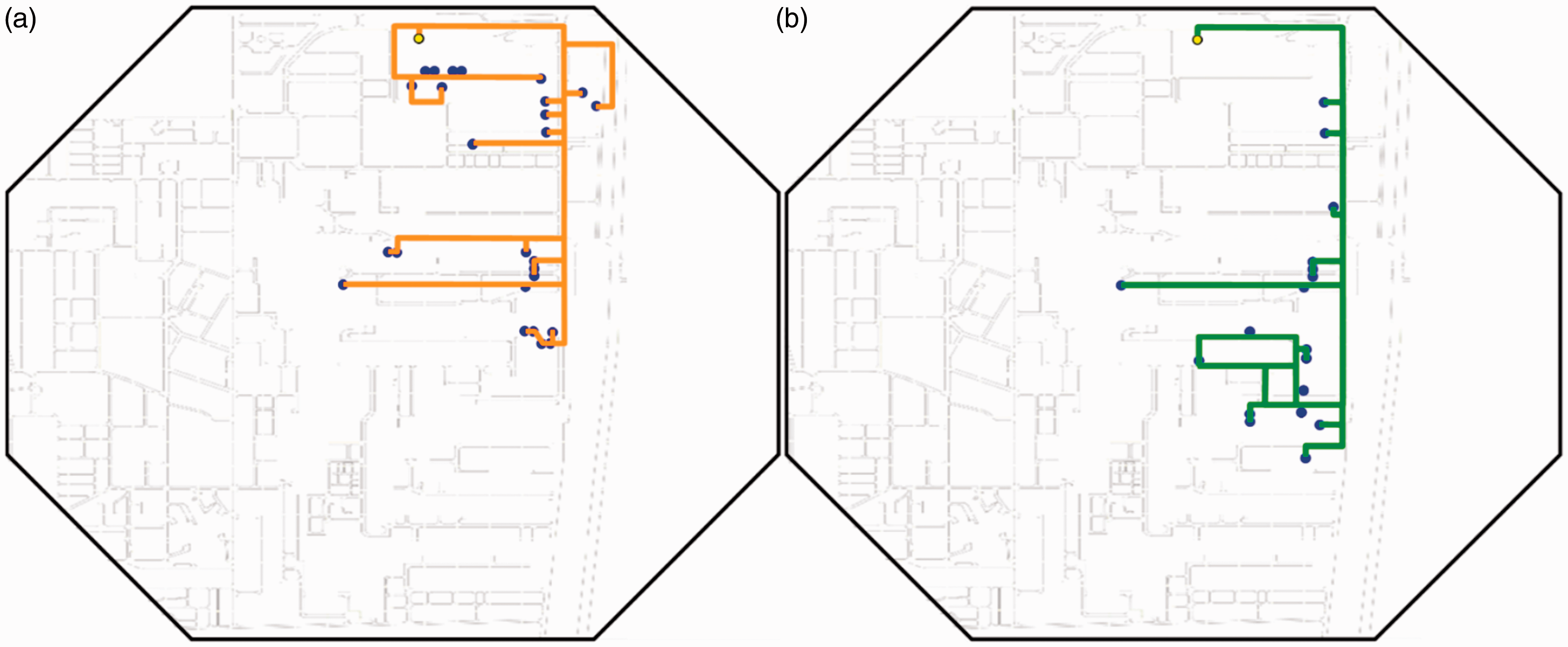
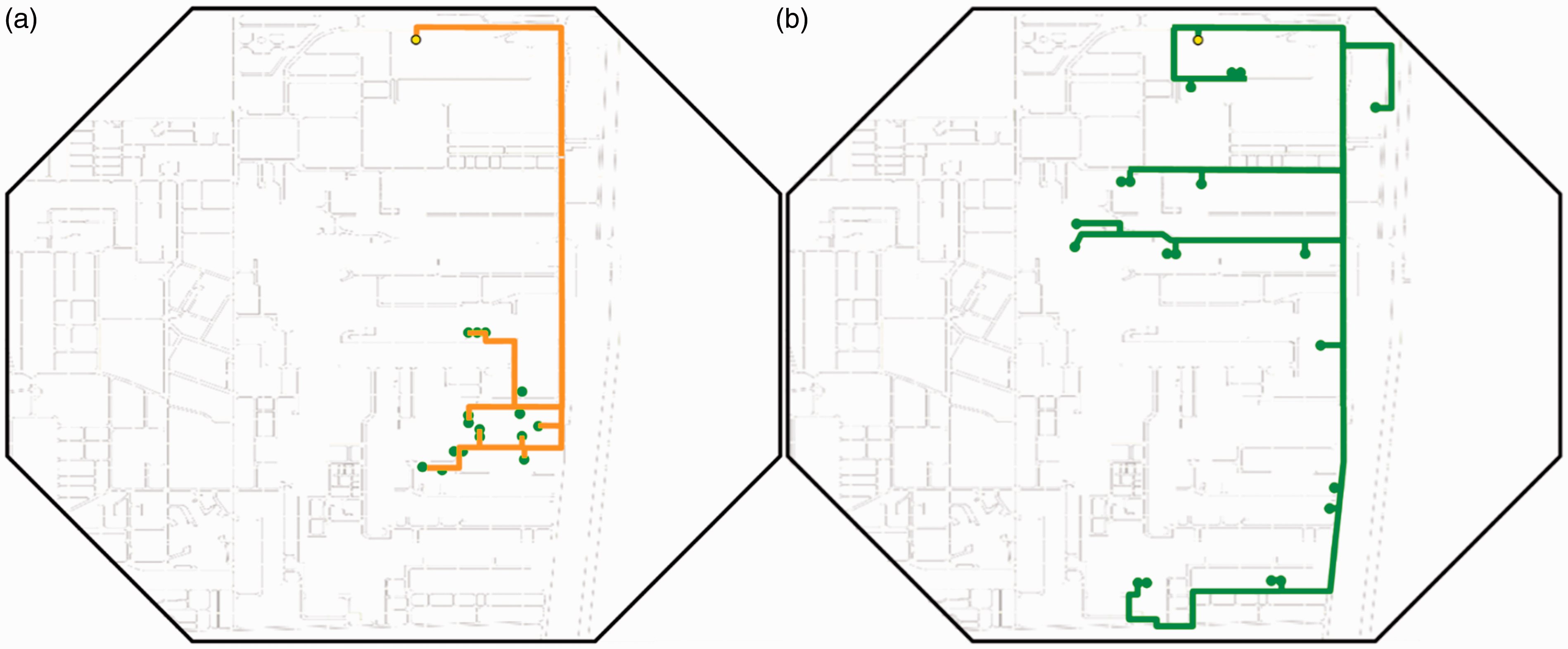
Artificial partition and AI six districts of the loading container configuration: (a) Manual and (b) DLGA.

Figure 17.

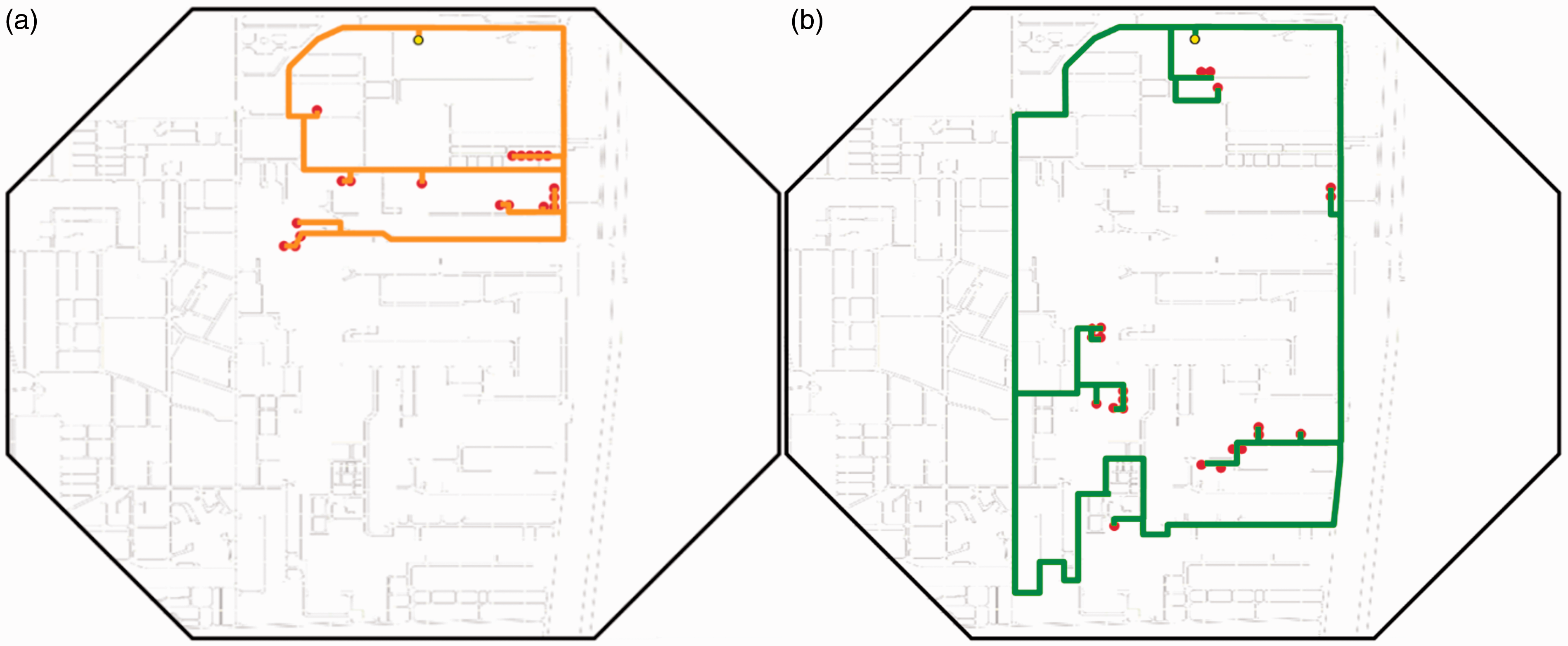
First districts of transport route: (a) Manual and (b) DLGA.

Figure 18.

Second districts of transport route: (a) Manual and (b) DLGA.

Table 4.

DLGA planning Pareto Analytic Solution of six districts.

	Total transit time	Partition time standard deviation	MAX.	MIN.
Manual planning	1372.85	22.13	261.10	200.00
DLGA Planning _A	1376.42	3.43	232.38	222.95
DLGA Planning _B	1351.86	27.55	260.26	189.80
DLGA Planning _C	1363.68	5.03	232.79	218.79

Table 5.

C solution and artificial partition transportation time comparison.

	Manual planning		DLGA solution
	Transport time of loading container – recycling yard	Transport time of loading container – loading container	Transport time of loading container – recycling yard	Transport time of loading container – loading container
First district	231.47	29.63	193.66	31.90
Second district	182.88	33.38	202.57	30.22
Third district	191.05	26.72	183.57	43.62
Fourth district	217.80	27.95	185.96	45.94
Fifth district	188.59	43.38	180.82	37.97
Sixth district	128.39	71.60	193.62	33.84
Standard deviation	35.62	17.17	8.08	6.42

DLGA: double-layer genetic algorithms.

Table 6.

Artificial planning five district for First shift schedule.

Item times	First district	Second district	Third district	Fourth district	Fifth district	Sixth district
1	P	P	P	P	–	P
2	A01	B01	C01	D01	–	F01
3	A02	B02	C02	D02	–	F02
4	A03	B03	C03	D03	–	F03
5	A04	B04	C04	D04	–	F04
6	A05	B05	C05	D05	–	F05
7	A06	B06	C06	D06	–	F06
8	A07	B07	C07	D07	–	F07
9	A08	B08	C08	D08	–	F08
10	A09	B09	C09	D09	–	F09
11	A10	B10	C10	D10	–	F10
12	A11	B11	C11	D11	–	F11
13	A12	B12	C12	D12	–	F12
14	A13	B13	C13	D13	–	F13
15	A14	B14	C14	D14	–	F14
16	A15	B15	C15	D15	–	F15
17	A16	B16	C16	D16	–	F16
18	A17	B17	E05	E09	–	E11
19	A18	B18	E01	E10	–	E12
20	A19	B19	E02	P	–	E13
21	E06	B20	E03		–	E14
22	E07	B21	E04		–	F17
23	E08	B22	P		–	F18
24	E15	B23			–	P
25	E16	B24			–
26	P	B25			–
27		B26			–
28		E17			–
29		E18			–
30		E19			–
31		E20			–
32		E21			–
33		P			–
Working time (min)	347.59	285.96	259.94	264.79	–	222.60

Quadrant I area: the total transport time and partition transport time standard deviation in the artificial partition results are poor, falling into this area solution without reference value.

Quadrant II: The total transportation time of solution B is lower than that of artificial partitioning, but the standard deviation of transport time in partitioning is worse than that of artificial partitioning, and the total transportation time is the best value of all solutions of DLGA.

Quadrant III: C solution of the total transport time and partition transport time standard deviation are lower than the results of artificial partition, the ideal solution area.

Quadrant IV: The total transportation time of solution A is higher than that of artificial partitioning, but the standard deviation of transport time in zoning is better than that of artificial partitioning, and it is the best value of all solutions.

Comparison between manual partition and DLGA solution

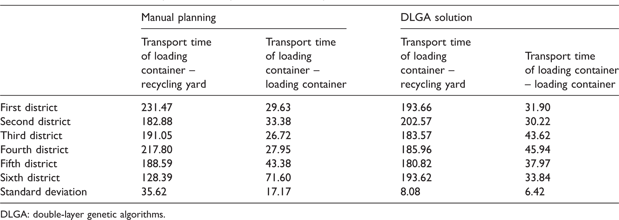
Artificial zoning has many years of accumulated practical experience; similar gene algorithms have evolved iterative process: the total transport time was 1372.85 min, and partition transport time standard deviation of 22.13 min, with considerable trustworthiness. After the relevant parameters are set and the program is optimized, the AI partition can gradually approach the status of the manual partitioning operation and even surpass the current status, obtaining the ideal solution of the total transport time of 1363.68 min and the standard deviation of the transport time of the partition in 5.03 min.

The standard deviation of transport time in DLGA partition was 17.1 min less than that of manual partitioning, and the improvement range was 77.3%. The total transport time of DLGA was 9.17 min less than the total transport time of artificial transport, with an improvement of 0.7%. Obviously, the case companies for the total transport time and the standard deviation of the transport time partition are two goals with the total transport time as the first. From another perspective, this is a multi-objective optimization problem; the artificial way to deal with such problems does have its own difficulties as only one treatment can be chosen.

DLGA partition can be obtained by the partition of the shortest transport path to reduce the total global transit time. Artificial zoning subarea transport path by the pilot according to experience means a long time trial and error mode work, similar to the Ant Colony Optimization solution mode; a shorter path means more vehicles running, the equivalent of ants in the path of residual pheromones content will be more numerous, and finally we will follow the residual pheromone content of the best path to travel, so the total transport time is higher than the DLGA partition, However, it is still quite competitive. However, this vehicle journey has accumulated experience and has not been standardized. New driving is subject to a considerable learning curve and takes some time to re-optimize the optimal route when the demand point changes.

The standard deviation of transportation time and the total transportation time of the subareas belong to the multi-objective optimization problem, and there are contradictions between the two. For example, the total transportation time of solution B is 1351.86 min, and the standard deviation of transportation time is 27.55 min. The standard deviation of transport times is 3.43 min and 5.03 min, respectively. Total transport time is higher than in the B solution. In Figure 15, the main effect map shows that the lower the standard deviation of transportation time in zoning, the higher the total transportation time will be. On the other hand, if the standard deviation of transportation time in zoning increases, the total transportation time will be moderately reduced.

The artificial partition cannot solve the NP-Hard problem in a reasonable time, so the difficult problem needs to be simplified to reduce the job complexity. Therefore, the partitioning is divided by the demand point geographical location; while the AI solution is partitioned by the transportation time. Table 5 shows the standard deviation of zoning and recycling time, and zoning-transportation time of zoning is greater than in the C solution.

The artificial partition divides the area by the geographical location of the loading demand points and the DLGA partitions the transport time. The results of the partitioning between the two are shown in Figure 16. The distribution results of the loading demand points of the artificial partition and the AI partition are obviously different from the transport path graph. However, from the perspective of the A1 zoning map, the loading on the Dead End Road can only be divided into a maximum of two zones. The operation of the two vehicles avoids the traffic congestion problem caused by the excessive allocation of vehicles on a single road. Most of the subareas have been grouped in order to avoid the destruction of the shortest path to achieve the same purpose as that of the artificial sub-area. The transport paths of the artificial sub-areas are shown in Figures 17 to 20 of the AI sub-areas. The transport path does not include loading demand points to the recycling field path.

Artificial planning of the five-zone transport schedule is shown in Table 6. The production line adjustment for the five-zone operation, due to the artificial partition, cannot be calculated by the partition transport time, only the original six districts of the fifth district loading demand points, to avoid the destruction of the shortest path are split to other districts; the total transport time was 1380.88 min, with partition transport time standard deviation of 45.99 min. However, the total transportation time of the five districts obtained by AI partitioning was 1349.79 min, and the standard deviation of transportation time by districts was 4.40 min, all of which were far better than the results of artificial partitioning.

Analysis of results from one to six zones of case companies

In using DLGA to solve the total transport time between the first and sixth regions and comparing them with the AI-C solutions, as shown in Table 7, the total transport time gradually decreases with the number of partitions. The greater the number of partitions, under the condition that a car is deployed in each district, the more on-line work vehicles, the relative increase in the round-trip distance between the parking lot and the loading points will increase the total transportation time. In addition, the assessment of the total transport time in the four-quarter operation was 1304.84 min and the conversion required for each vehicle was about 5.44 h. This exceeded the operating condition limit of 5 h or less per transport service per class. Obviously, planning the first quarter to the fourth quarter will not be able to meet the existing transport needs under the current operating conditions of the existing individual companies under the preconditions of operating conditions.

Table 7.

AI solution results for one to six district.

AI solution results(H)	Total transit time	transit time for each vehicle
AI Planning _C_6 district	1363.68	3.79
AI Planning _C_5 district	1349.79	4.5
AI Planning _C_4 district	1304.84	5.44
AI Planning _C_3 district	1295.48	7.2
AI Planning _C_2 district	1283.28	10.69
AI Planning _C_1 district	1251.12	20.85

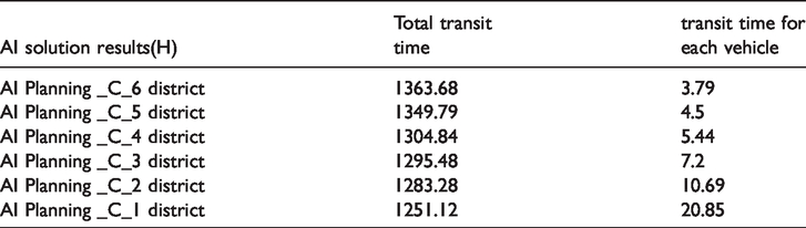
In addition, from the analysis of the number of zones in Figure 20 and the total transit time, it is obvious that the number of zones shows a positive correlation with the total transport time. With the increase in the number of zones, the total transport time also increases. In addition, a straight line passing through these two points is drawn on the basis of the total transit times of one and two subzones, with which the total transit time required under each of the subzones can be predicted; however, the solution shows that the total transport time of three to six districts located on the right side of the line, that is, under the number of partitions, obtained by AI is lower than the expected total transport time, indicating that AI can really obtain the better forecast solution.

Figure 19.

Third districts of transport route.

Figure 20.

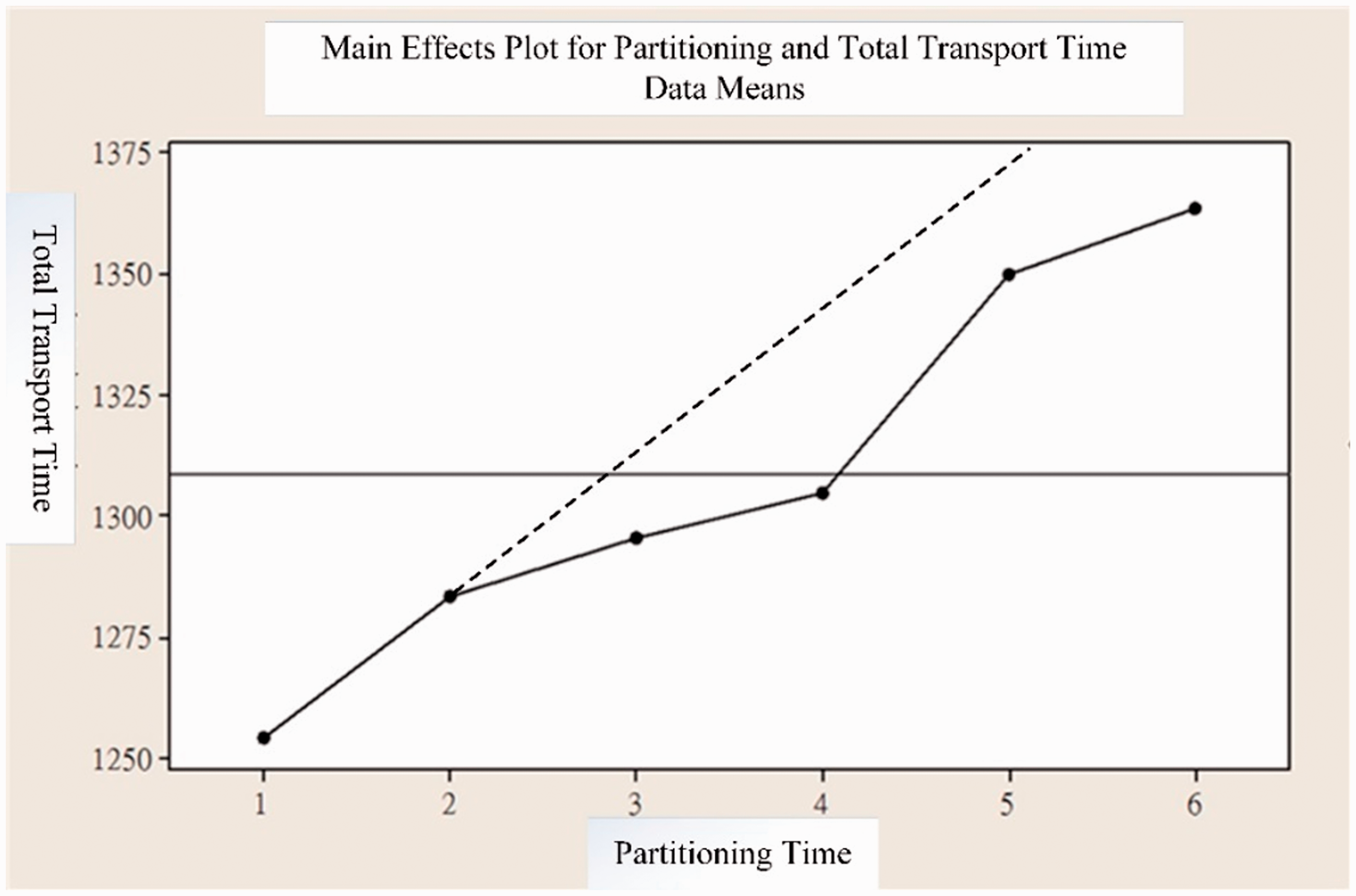
Effect analysis of partitioning and total transport time.

Conclusion

In this study, checkerboard foam gene chromosomes can effectively solve the problem of vehicle zoning operations, simplify the complexity of gene evolution, and enhance the efficiency of the solution. Then, with artificial zoning planning operations similar to the gene algorithm, and the transport route by district to find the best path by driving, is similar to the ant colony algorithm; after a long period of evolution, it can still get a reasonable total transit time, but the cost of manpower and material resources cannot be underestimated. The AI assistance built through this study can effectively enhance the planning efficiency and can provide the best loading schedule and total transport time of each subarea after planning to avoid driving on an individual basis of habits or experience planning transport routes, to reduce transportation costs.

Moreover, the total transport time and partition transport time standard deviation contradictory to the proposed DLGA method can be calculated for deriving the best total transport time solution and the best partition transport time standard deviation, with the results being available as a decision-making reference: select the minimum total transit time or partition transport, and minimize the time difference, depending on the industry considerations. The minimum total transport time can effectively reduce transportation costs, but the zoning operation time is quite different. To avoid uneven service, periodic rotation can be adopted. In the long run, it can effectively reduce the difference of labor for each driver and allow all drivers to drive with familiar zoning operation characteristics, to avoid leaving and resulting in having more standby manpower available for scheduling, thereby reducing management problems. In the future, consideration may be given to introducing loading requirements into the computer reservation system so as to grasp the demand situation before the departure of each shift and instantly plan the best zoning transport to effectively reduce transportation costs and to make the driving transportation time more even.

Footnotes

Acknowledgements

The authors would like to thank Mr Hsieh, anonymous reviewers, and the associate editor for their constructive suggestions which helped improve the quality of this paper.

Declaration of conflicting interests

The author(s) declared no potential conflicts of interest with respect to the research, authorship, and/or publication of this article.

Funding

The author(s) disclosed receipt of the following financial support for the research, authorship, and/or publication of this article: This work is supported by Ministry of Science and Technology (MOST) of Taiwan, under Grant number MOST 107–2221-E-992–092.

References

Flood

MM.

The traveling-salesman problem. Oper Res 1956; 4: 225–330.

Applegate

Bixby

Chvátal

, et al. The traveling salesman problem. Princeton, NJ: Princeton University Press, 2007.

Toth

Vigo

Vehicle routing: Problems, methods, and applications. Philadelphia, PA: SIAM Publications, 2014.

Bodin

, et al. Routing and scheduling of vehicle and crew: the state of art. Comput Oper Res (Special Issue) 1983; 10: 63–211.

Gendreau

, et al. Vehicle routing: problems, methods, and applications, stochastic vehicle routing problems, Chapter 8. Mathematical Optimization Society, Philadelphia, 2014, pp. 213–240.

Cattaruzza

, et al. A Memetic Algorithm for the multi trip vehicle routing problem. Eur J Oper Res 2014; 833–848.

Ongarj

Ongkunaruk

An integer programming for a bin packing problem with time windows a case study of a Thai Seasoning Company. In: 10th International conference on service systems and service management, pp.826–830. Piscataway, NJ: IEEE.

Popović

, et al. Fixed and flexible zoning strategies for parcel distribution in uncertainty environments. Transp Logist 2013; 13: 1–8.

Crainic

, et al. Multi-zone multi-trip VRP with time windows. Inf Syst Oper Res 2015; 53: 49–67.

10.

Yang

Path planning based on double-layer genetic algorithm. In: IEEE 3rd international conference on natural computation, Haikou, China, 24–27 August 2007.

11.

Sikora

Shaw

A double-layered learning approach to acquiring rules for classification: Integrating genetic algorithms with similarity-based learning. J Comput 1994; 6: 107–220.

12.

Dobric

Durisic

Double-stage genetic algorithm for wind farm layout optimization on complex terrains. J Renew Sustain Energy 2014; 6: 1–1200.

13.

Sungur

The robust vehicle routing problem. PhD Dissertation, Faculty of The Graduate School University of Southern California, USA.

14.

Kim

Weck

OD.

Variable chromosome length genetic algorithm for structural topology design optimization. In : 45th AIAA/ASME/ASCE/AHS/ASC structures, structural dynamics & materials conference, Palm Springs, CA, 19–22 April 2004.