
Abstract
In this study, a new methodology, hybrid Strength Pareto Evolutionary Algorithm Reference Direction (SPEA/R) with Deep Neural Network (HDNN&SPEA/R), has been developed to achieve cost optimization of stiffness parameter for powertrain mount systems. This problem is formalized as a multi-objective optimization problem involving six optimization objectives: mean square acceleration of a rear engine mount, mean square displacement of a rear engine mount, mean square acceleration of a front left engine mount, mean square displacement of a front left engine mount, mean square acceleration of a front right engine mount, and mean square displacement of a front right engine mount. A hybrid HDNN&SPEA/R is proposed with the integration of genetic algorithm, deep neural network, and a Strength Pareto evolutionary algorithm based on reference direction for multi-objective SPEA/R. Several benchmark functions are tested, and results reveal that the HDNN&SPEA/R is more efficient than the typical deep neural network. stiffness parameter for powertrain mount systems optimization with HDNN&SPEA/R is simulated, respectively. It proved the potential of the HDNN&SPEA/R for stiffness parameter for powertrain mount systems optimization problem.
Keywords
Introduction
Multi-objective evolutionary algorithms (MOEAs) are common tools for solving multi-objective optimization problems in the technical field, because of their performance on issues with large design spaces and scenes difficult exercise. Inside, SPEA2 (Intensity 2 Evolutionary Algorithm) is used to evaluate the Pareto solution due to the good performance of a variety of solutions different from normal multi-objective reliability assessment. There are some researchers on this field like De Tommasi et al. 1 who have proposed a multi-objective optimization for RF circuit blocks through replacement models and NBI and SPEA2 methods. Sofianopoulos and Tambouratzis 2 proposed a model-based machine translation system using large monolithic blocks in the target language from which statistical information was extracted. This study reported using a specific machine translation to represent the test that SPEA2 was chosen as the optimization method. Zhao et al. 3 proposed an SPEA2 algorithm based on adaptive selection evolutionary operators (AOSPEA). The proposed algorithm can selectively adapt simulated binary interference, polynomial mutations, and differential evolutionary operators in their evolution according to their contribution to the external repository. Ben Hamidabrini Salah et al. 4 proposed the Pareto Strength (SPEA2) Evolution Algorithm for the Economic/Environmental Power Distribution (EEPD) problem. In the past, minimizing fuel costs was the only objective function of economic power coordination. Due to the modification of clean air behavior has been applied to reduce emissions of polluting emissions from power plants, utilities have also changed strategies to reduce pollution and atmospheric emissions, minimizing generation waste when other target functions turn economic capacity (EPD) into versatile-objective problem with conflicting goals. Jiang et al. 5 published a new SPEA based on the reference direction, denoted SPEA/R, to optimize multiple goals. A significant extension of the early SPEA algorithms is SPEA/R. It applies to the advantage of SPEA2’s physical assignment in quantifying solutions diversity and convergence in one method. It is appropriate to replace the most time-consuming density estimator with an algorithm based on the reference direction. Their proposed exercise duties also take into account the convergence both local and global. However, MOEAs algorithms still need a lot of computational time to evaluate the objective function in the typical practical problem-solving process. When the problem is more difficult and complicated, the calculation time will be longer. Combined, this could make the use of MOEAs algorithms impractical. Therefore, the best way to reduce computation time is to use artificial neural networks (ANNs) with multiple hidden layers plus deep learning algorithms to accelerate calculations.
The ANNs with hidden layers combined with deep learning algorithms is one of the most widely used and accurate predictive models. Many researchers have applied this method in the areas such as economics, engineering, society, foreign exchange, securities issues, etc.6–14 The application of neural networks in predictive models optimizes many goals based on the ability of neural networks to predict that non-fixed behavior is very accurate. For traditional mathematical models or statistical models, it is inconsistent with unusual data patterns that cannot be clearly written as functions or deduced from a formula, while ANN algorithms can work with chaotic components. Currently, there are a number of researchers such as Shen et al., 15 who have come up with potential uncertainties of wind power and have since proposed options for building intervals prediction (PI) with predictive models using wavelet neural network, in which the upper and lower limit estimate of PI has been implemented by minimizing the multi-objective function including the probability of span width and coverage range. Smith et al. 16 announced a recurrent neural network used as an alternative method to predict long-term models of fluid dynamics simulation in computation. In particular, hybrid MOEAs have been trained and optimized structures from introduced recurrent neural networks. Kakaee et al. 17 published a method of using ANNs followed by multi-objective optimization using NSGA-II evolution algorithm and SPEA2 optimization algorithm to optimize the operating parameters of a compression ignition heavy-duty diesel engine. Vieira and Tome 18 published two different methods to increase the search speed of the multi-objective evolution algorithm (MOEA) using ANNs.
In this article, a new hybrid optimization algorithm is proposed for multi-objective problems. This is the hybrid between the genetic algorithm (GA), deep neural network (DNN), and strength Pareto evolutionary algorithm-based reference direction for multi-objective (SPEA/R) to find the best of the Pareto-optimal front. This combination gave computing time much faster than computing time when using GAs SPEA/R. On the other hand, this combination also significantly reduces the number of samples needed for the training of deep ANNs. The performance of the new algorithm is demonstrated via some complex benchmark functions and for powertrain mount system stiffness parameter optimization problem with six-objective optimization in model 3D.
The organization of this article is as follows: section “structure” describes the proposed new hybrid HDNN&SPEA/R method and the vibration characteristic of the powertrain mount system. Section “simulation results and discussion” describes simulation results of application HDNN&SPEA/R method to computational experimentation with several benchmark functions and optimization of the powertrain mount system stiffness parameter. Finally is a conclusion.
Structure
Many-objective optimization SPEA/R algorithm
Jiang et al. proposed SPEA/R algorithm as presented in the flowchart in Figure 1.
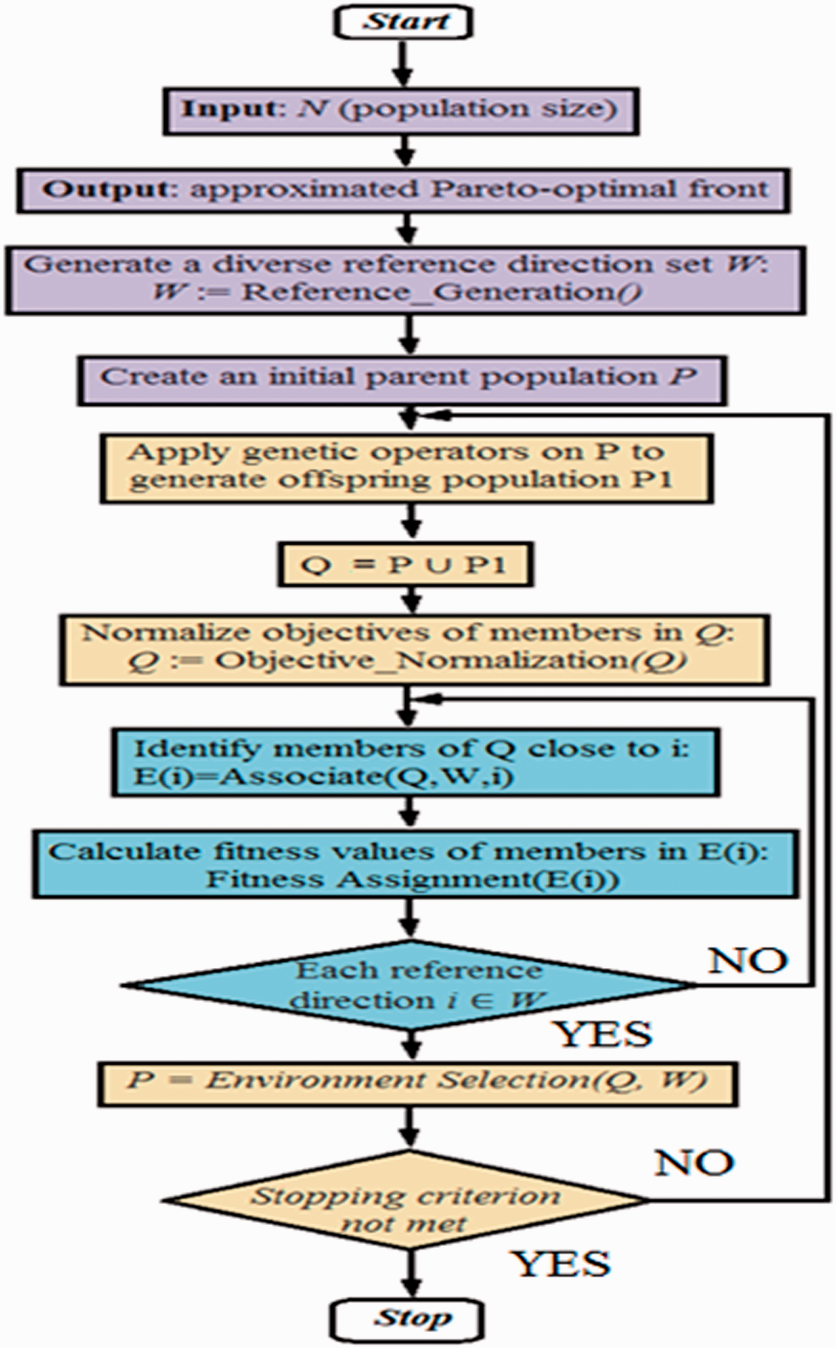
Flowchart of SPEA/R.
New hybrid HDNN&SPEA/R method
DNN
ANNs are simulations of simplified models of the human brain. They have the ability to estimate complex nonlinear relationships between corresponding input and output data parameters. 19 As shown in Figure 2, the neural network has a link structure consisting of three types of classes. It is an input layer, hidden layer, and output layer. Each network layer consists of a number of neurons and is organized into layers, in which the nerve cells of different layers in the network are connected by connections connected to independent weights (Wi). In addition, an independent bias (b) can be added to each neuron. On the other hand, the transfer function determines the influence of the weights and biases of the neuron on the neurons of the next layer and can be linear or nonlinear. In addition, there are several types of transfer functions (such as pureline, logig, and tansig); some neurons and some hidden layers are hyperparameters of neural networks to create different structures of the network. neuron. Finally, weights and biases adjustment process are called the network training process, and they are usually evaluated by minimizing the average mean square error (MSE) between the predicted outputs of the neural network and the output reality.
Figure. 2. The architecture of a feedforward artificial neural network with M neurons in input, N in hidden layer, and K in output layers.
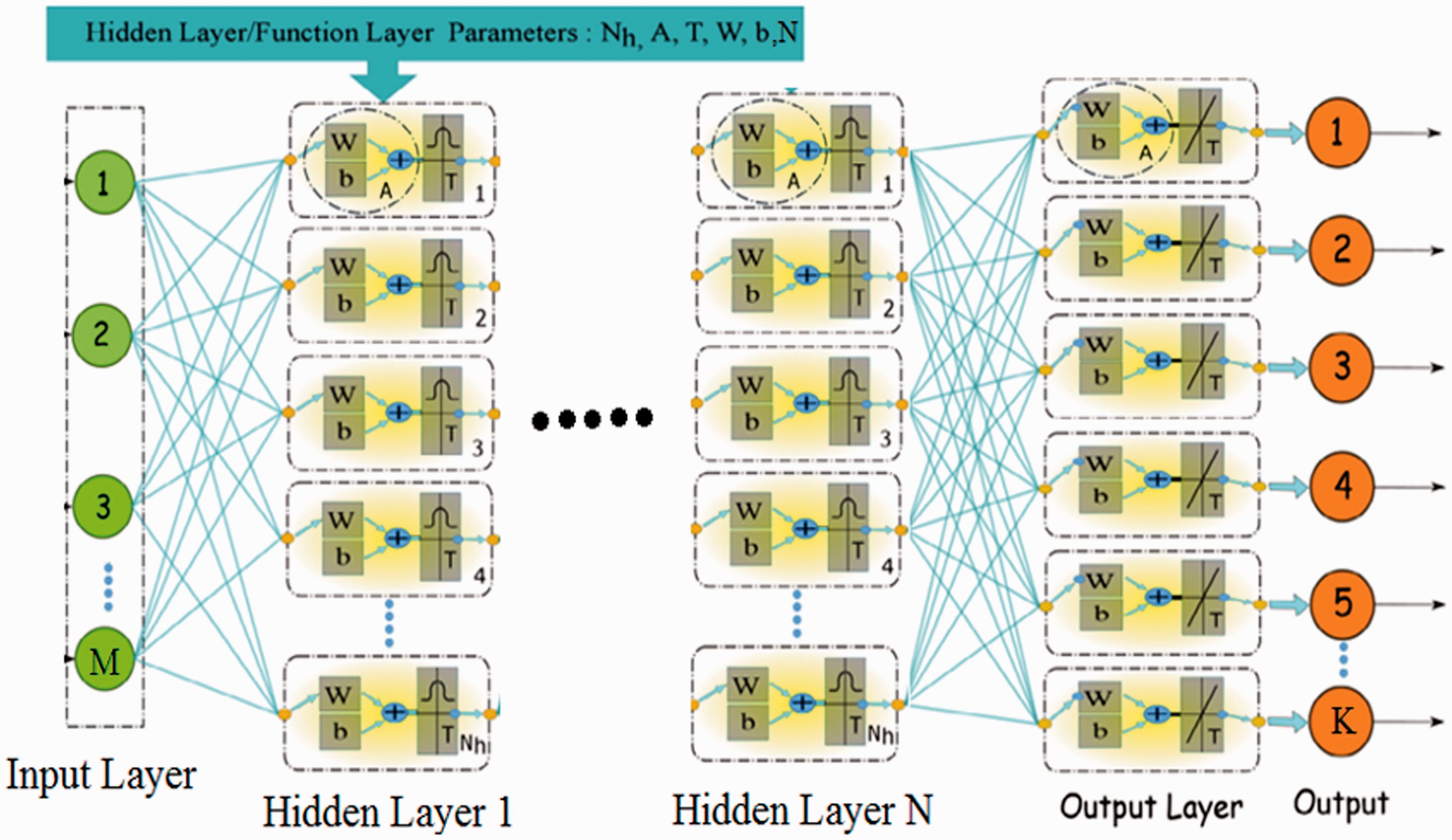
In this article, we use the multilayer perceptron (MLP) neural network structure. MLP is a feedforward ANN defined by an input layer with M neurons. N layers hidden, in which each hidden layer has Nh number of neurons and an output layer has K neurons. In the MLP network structure, each layer has full connections to the next layer, which means that each neuron output in layer N is the input of each neuron in the N + 1 layer. Figure 2 shows one example of an MLP network with input neuron M, N hidden layer with each hidden layer has Nh neuron, and the output layer has K neurons. MLP network can be described with: nn = (M Nh1 Nh2 … NhN K).
DNN optimize
Recently, some researchers have published some new effective methods to train ANN neural networks, in which the weights and biases of neural networks are optimized by GA algorithm.
20
In the process of network training, GA finds weight and bias values quickly and optimally for neural networks. That makes the number of iterations in network training greatly reduced. Thus, the time for training is faster. Besides, the global ability of searching and evolution of parameters is a key feature of GA. Therefore, GA was introduced in this study. This method uses the theory of natural selection and biological evolution. It is the choice, cross-exchange, and mutation of individuals to select the best and most suitable member. The initial weight and bias of DNN have been evolved in the process of training neural networks. The interaction between the GA and DNN is done through weight and bias exchange. The DNN was started to get a random weight and biases (Wi and b) as shown in Figure 3. This is the initial population included in the GA algorithm. Then, the next generation is generated by the GA based on the current population. To evaluate the difference between the predicted output values and the actual output values, it is used as the fitness function. Decide on acceptable parameters if the total average square of GA is less than 0.005. Weight and biases are calculated by the equation (1)

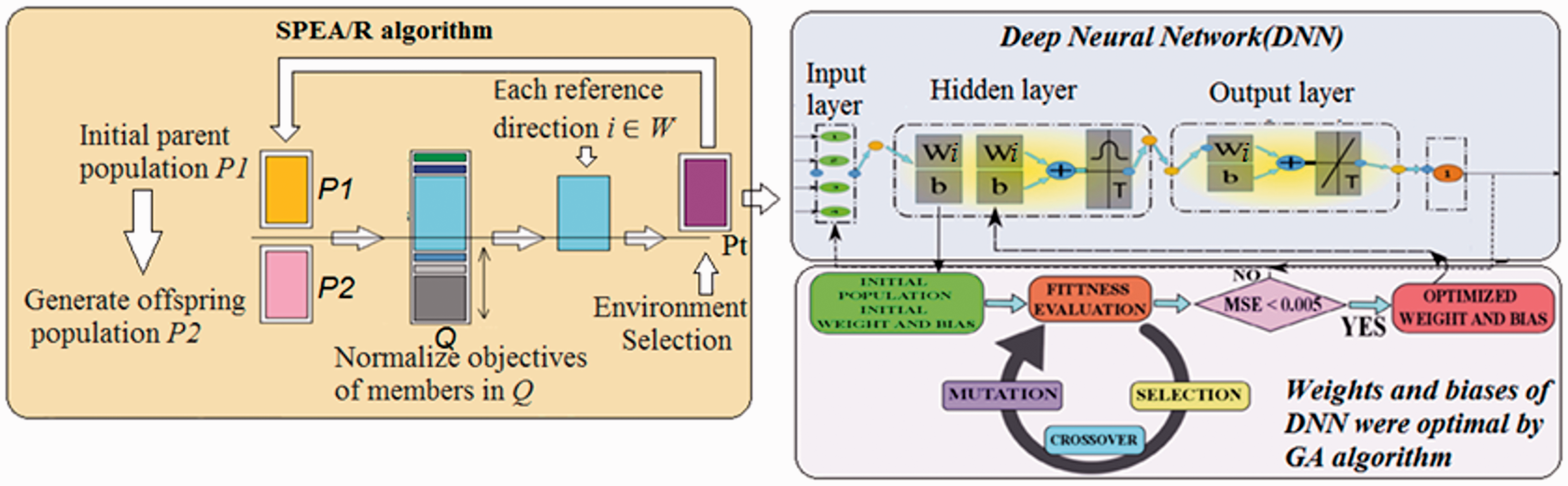
Training structure for hybrid method.
The deep learning training algorithm
The purpose of this section is to allow the DNN neural network to learn the optimal analytical characteristics of many objects from the SPEA/R algorithm. We have combined DNN training with the optimal analysis of SPEA/R algorithm as shown in Figures 3 and 4. This process started with the SPEA/R algorithm with a random population of input variables P1. After that, summing up the population Q at time t is created by population P1 and population P2 (where P2 is generated from P1 parents’ population through the use of conventional genetic operators such as selection, mutations, and cross exchanges). After that, all individuals were combined into population Q.
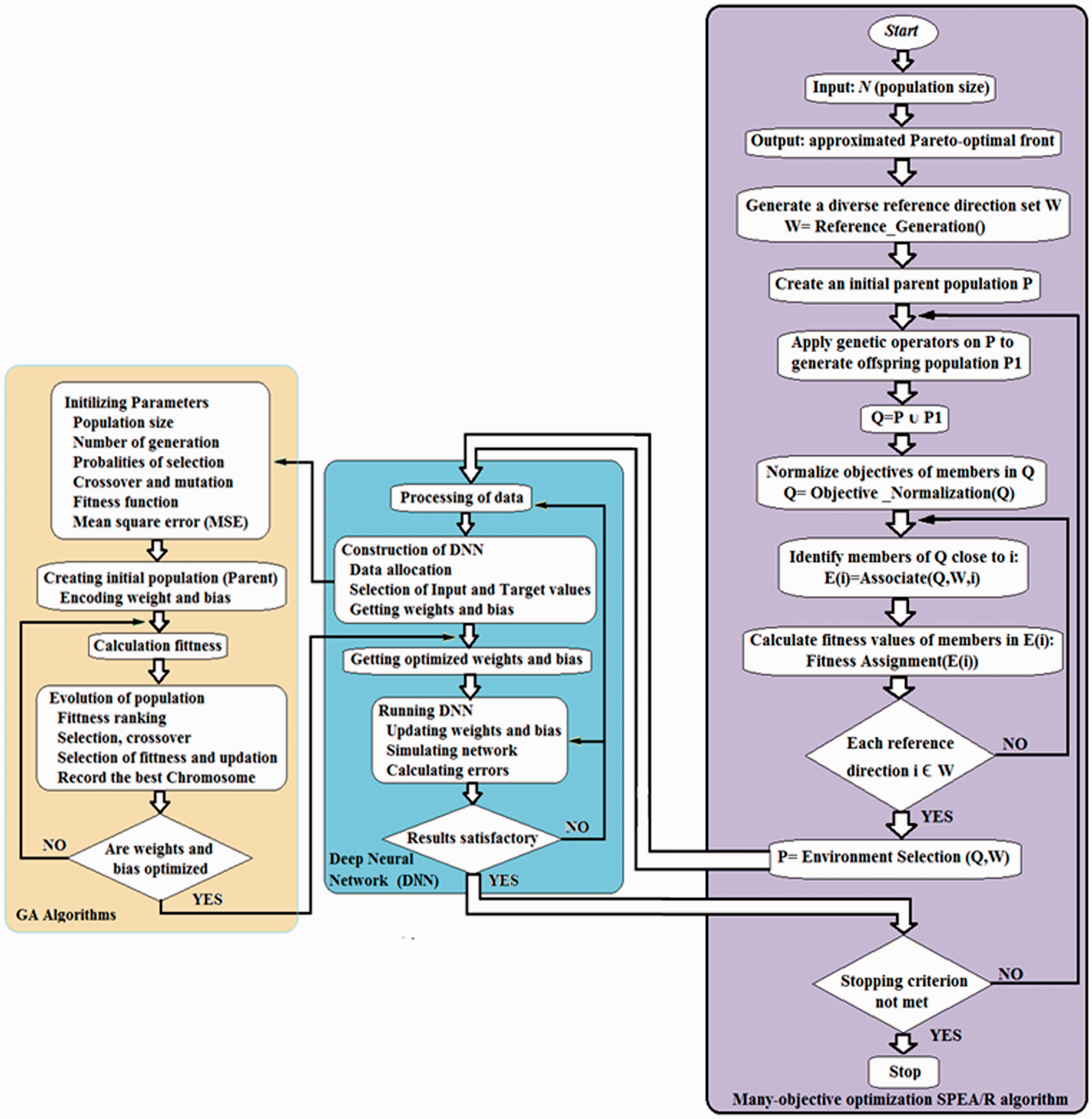
Training algorithm.
From this population, individuals were selected to enhance reproduction instead of random selection. It is therefore very useful for optimizing many goals when remote parents are unable to create good solutions. The use of simple normalization based on the worst value of each SPEA/R goal deliberately gives higher priority to diversity than convergence when making environmental choices leading to printing performance for MOP issues. From there, the best Pareto fronts were selected (stored on the top of the list) and transferred to the new parent group Pt. Through this process, the most quintessential nuclei were selected. Since the size of the Pt population is only half of Q (in fact the size of Pt is equal to the size of P1), half of the Pareto front will be deleted during the transfer. This process will be continued until all individuals of a specific Pareto front cannot be completely provided in the parent population of Pt. Therefore, for choosing the exact number of individuals of that particular front for filling remained space of the population Pt, an associate population with reference points to keep a constant number of individuals (POP: population size). Finally, the population update process Pt will be used to replace population P1 in the next generation of the SPEA/R algorithm and the Pareto temporary front optimization will be defined after a specific generation can. Therefore, after each cycle of population update (Pt) in the SPEA/R algorithm, Pareto front temporarily will be transferred to the DNN including input data and output data (that is the Temporary Pareto front) to train the DNN. From here, we see a lot of Temporary Pareto front files created from the SPEA/R algorithm, which means there are many standard data sets for training DNN. Therefore, the combined training of the DNN has the full characteristics of the SPEA/R algorithm, but it has a fast calculation speed and converges faster of neural networks. The search area is larger than the SPEA/R algorithm because the DNN is trained on many standard samples. This process has been generalized according to Algorithms 1 and 2 as follows
1: Input: Pareto temporary front set
2: Output: weight and bias values optimized
3: Initializing parameters
Population size
Number of generation
Probabilities of selection
Crossover and mutation
Fitness function
Mean square error
4: Creating initial population parent encoding weight and bias
5:
6: Calculation fitness
7: Evolution of population
8: Fitness ranking
9: Selection crossover
10: Selection of fitness and update
11: Record the best chromosome
12:
1:
2:
3: Create a diverse set of reference directions F
F: = Reference Create ();
4: Create an original parent population P1;
5:
6: Apply this genetic operator P1 to create offspring
7: Q: = P1 ∪ P2;
8: Normalize the goals of internal members Q:
Q: = Objective normalization(Q);
9:
10: Identify members of Q close to i:
H(i) := Associate (Q, F, i);
11: Perform calculations fitness values of members in H(i):
Fitness assignment (H(i));
12:
13: Pt: = Choose the environment (Q, F);
14: Call
15:
Leave-one-out cross-validation (LOOCV) method
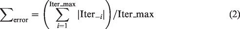
Cross-validation is the most common and effective way to verify models in statistical machine learning. This method is intended to estimate predictive models that they have learned from training data. How it will do on data that has not been tested in the future. In other words, by this method, we can measure the generalized power (accuracy) of our trained model in practice and avoid overfitting when the use of techniques in cross-validation. LOOCV is the most common cross-authentication method. This technique is often applied when the amount of training and testing data is not too large or too difficult to create a large training/test data set for model learning. With this method, in each iteration, a sample of the temporary data point is considered as the validation data and the remaining data is used for model training. Through each model training process, its prediction errors will be calculated on the validation data. If the initial training data contains Iter_max samples, this procedure repeats Iter_max times (it equals the number of observations in the initial training set). Then, the average of these errors is reported as the predictive error of our predictive model across the entire data set in terms of expressions by equation (2). Thus, with this validation method, in its iterations Iter_max, all patterns have the opportunity to act as a prototype. For more information on LOOCV, refer to Ron.
21
Vibration characteristic of the powertrain mount system
Full car model with 10 degrees of freedom (D.O.F.) is shown in Figure 5. Suspension and tires are considered spring and damping systems. Where the masses m2.1, m2.2, m2.3, and m2.4 denote the weight of four wheels (the mass does not burst). The masses mcg1 and mcab represent the mass (unburnt mass) of the frame and engine, respectively. Z3.1, Z3.2, Z3.3, and Z3.4 are the vertical displacements of the wheel, Z1, Z2 are, respectively, the vertical displacement of the frame and the transmission system. And, Roll and Altitude are vibrations that rotate around the corresponding X and Y axes. Next, the symbols Φ and Ψ represent the pitch and roll of the frame. The inertia of the transmission system on the y-axis and the x-axis are Iyy and Ixx, respectively, the inertial moment for the chassis on axes X1 and Y1 are Iyy1 and Ixx1, respectively. The stiffness and damping parameters of the wheels are K3.1, K3.2, K3.3, K3.4 and C3.1, C3.2, C3.3, C3.4, respectively. Similarly, the hardness and damping parameters of primary suspension are K2.1, K2.2, K2.3, K2.4 and C2.1, C2.2, C2.3, C2.4, respectively, while the hardness and damping parameters of the drive system are K1.1, K1.2, K1.3 and C1.1, C1.2, C1.3, respectively. The distance of the front and rear support from the center (CG) of the transmission system is a and b, respectively; the right and left mounting distances from the CG of the transmission system are c and d, respectively. a1, b1, c1, and d1 Distances for the chassis are indicated as follows.
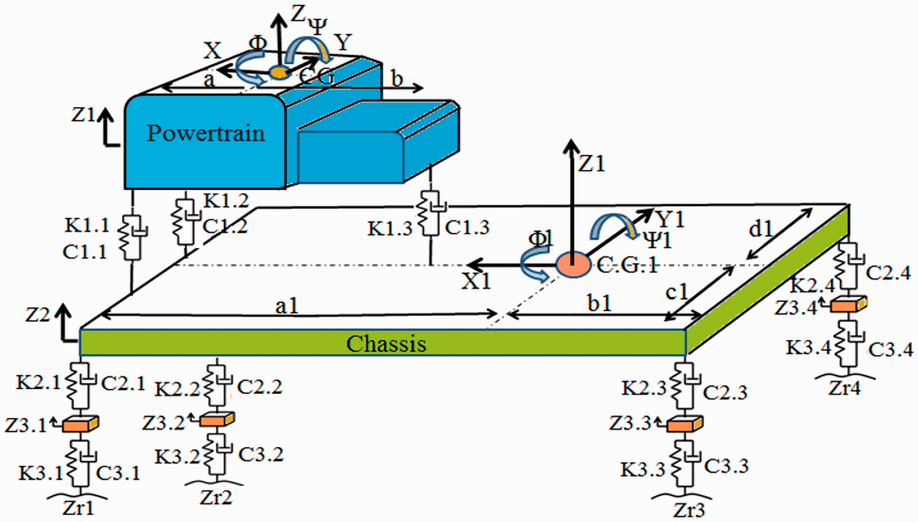
The principle diagram of a full-car dynamic model with a power source system mounting system.
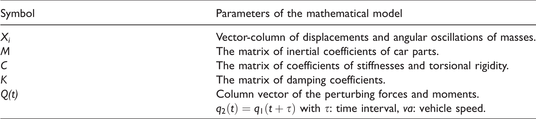
By using Newton’s law, the mathematical model of Figure 4 can be written as below

Parameters of the mathematical model.
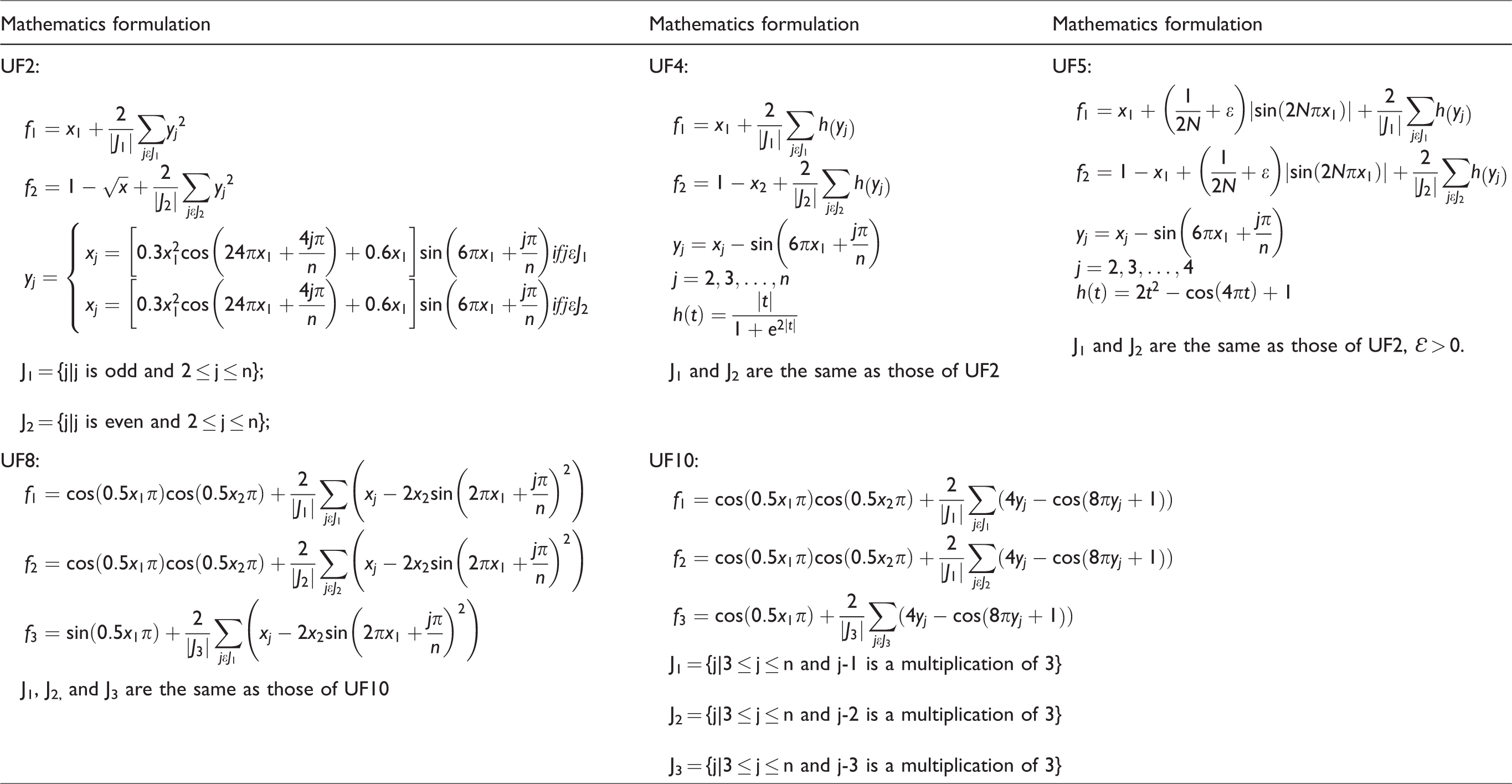
Benchmark Functions for test multi-objective optimization.
Simulation results and discussion
Numerical results
In this section, to demonstrate the superiority of the HDNN&SPEA/R method, we conducted calculations and tests on a number of benchmark functions. The results are compared to SPEA/R algorithms and Simplex NSGAII algorithms.
22
For the performance metric,
23
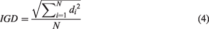
inverted generational distance (IGD),
24
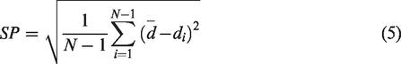
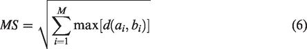
spacing (SP), and maximum spread (MS)
25
criteria are employed to measure convergence, quantity, and coverage, respectively. The mathematical formulation of IGD is as follows
In addition to utilizing the performance metrics, the best set of Pareto front optimal solution obtained by HDNN&SPEA/R on both the parameter space as well as the search space is shown in Figures 6 and 7. These figures show the performance of HDNN&SPEA/R in comparison with the true Pareto front, and at the same time it is compared with the results of Simplex NSGAII algorithms. For a comparative evaluation, all the algorithms are run 20 times on the test problems, and the statistical results of the 20 runs with algorithm parameters are provided in Table 3. Statistical results of the algorithm for IGD, SP, and MS are provided in Tables 4 to 6, respectively of benchmark functions. In Table 4, the IGD parameter is a performance indicator that shows the accuracy and convergence of the algorithm. The IGD parameter shows that the proposed hybrid algorithm (HDNN&SPEA/R) can provide better results than the Simplex NSGAII algorithm, but it is far more than the SPEA/R algorithm.
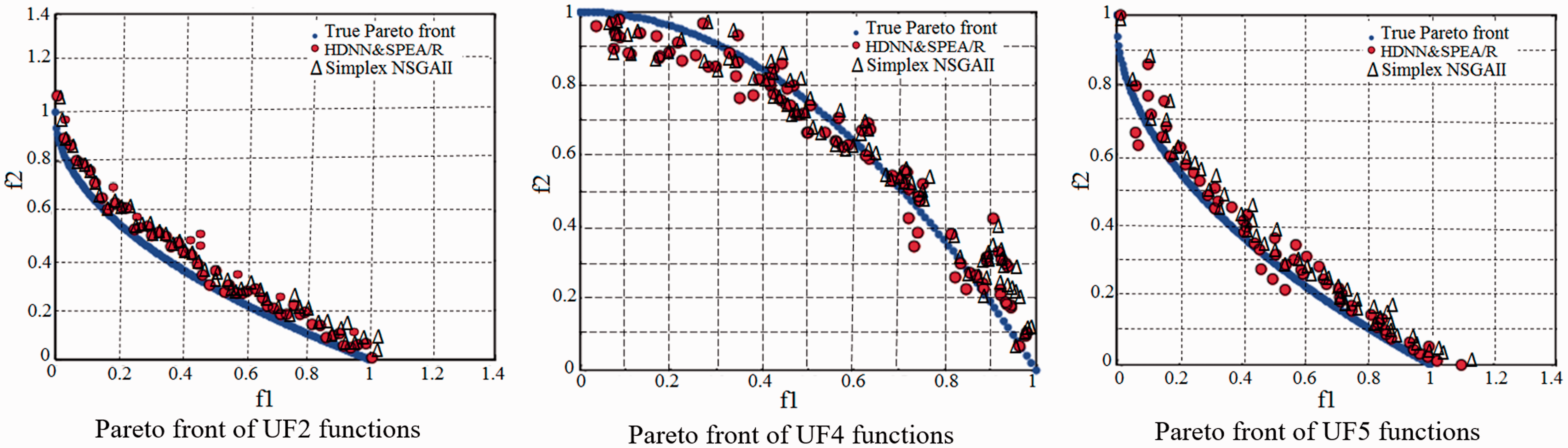
Pareto front set of bi-objective benchmark functions.
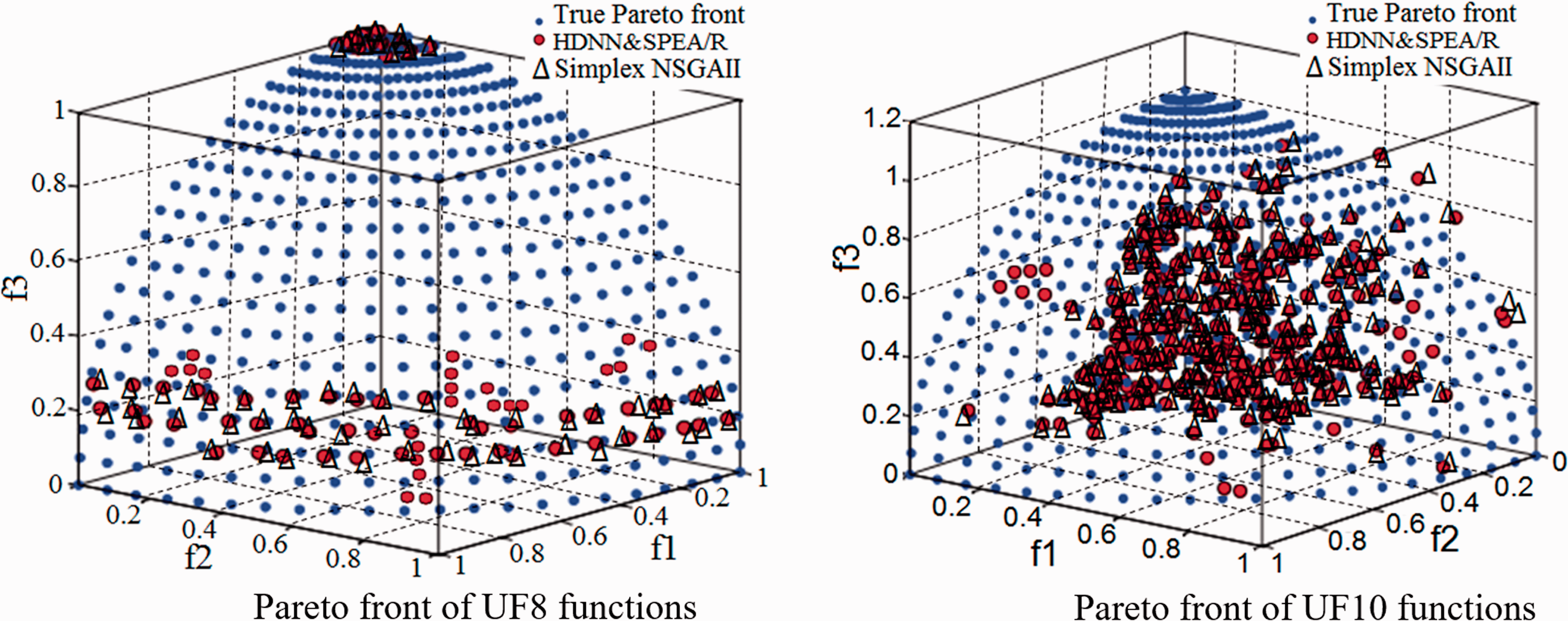
Pareto front set of tri-objective benchmark functions HDNN&SPEA/R.
Model parameters of SPEA/R algorithm and DNN
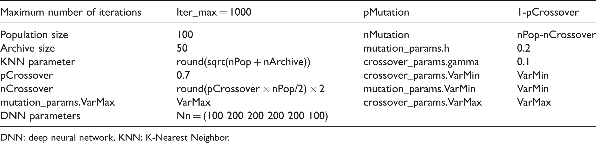
DNN: deep neural network, KNN: K-Nearest Neighbor.
Results for IGD.
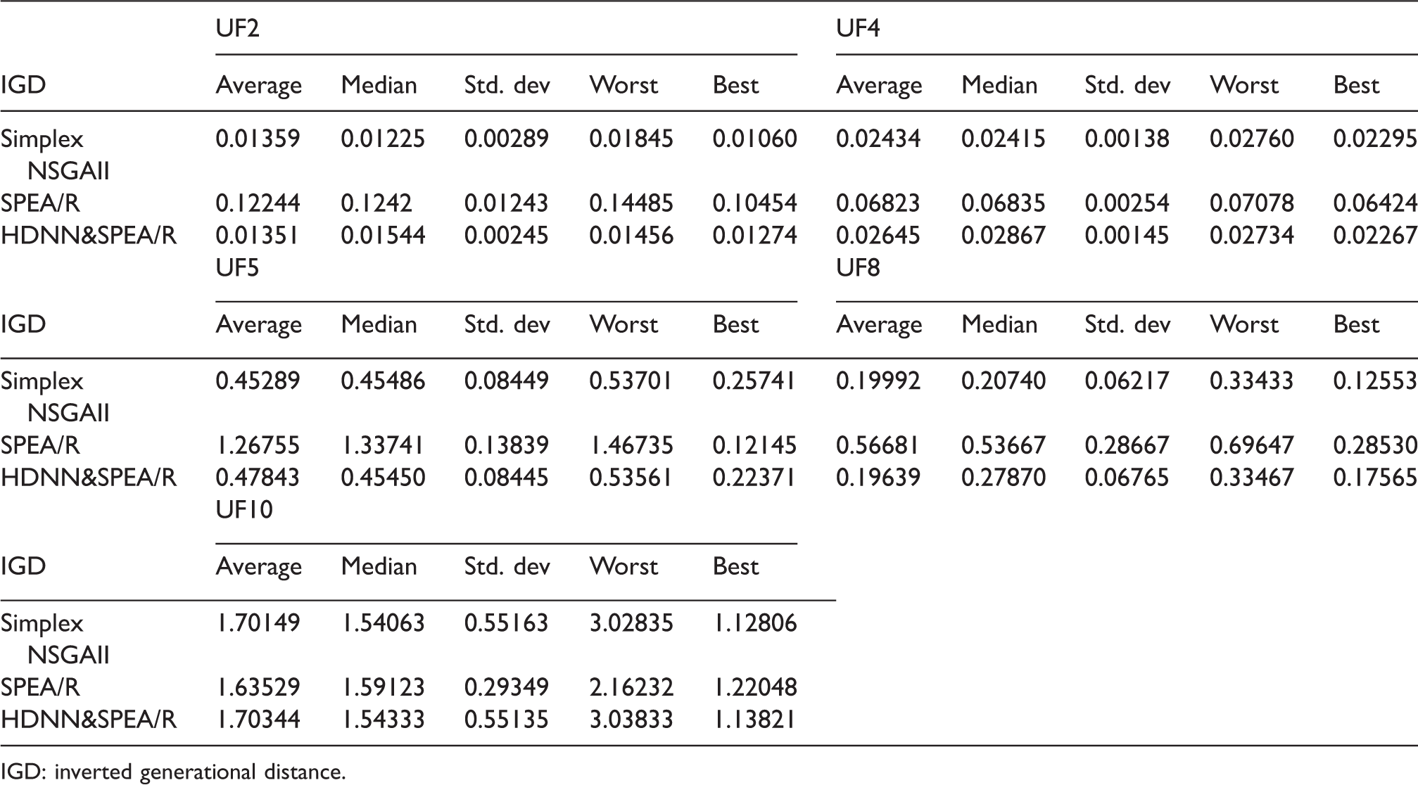
IGD: inverted generational distance.
Results for SP.
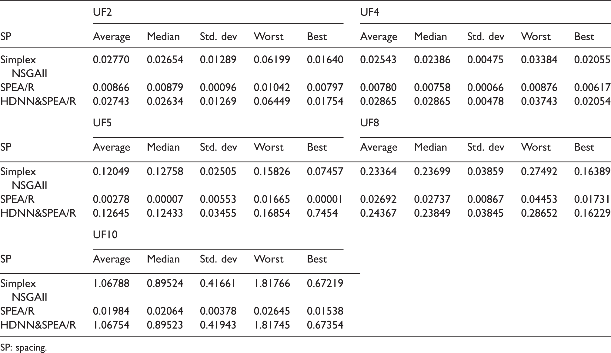
SP: spacing.
Results for MS.
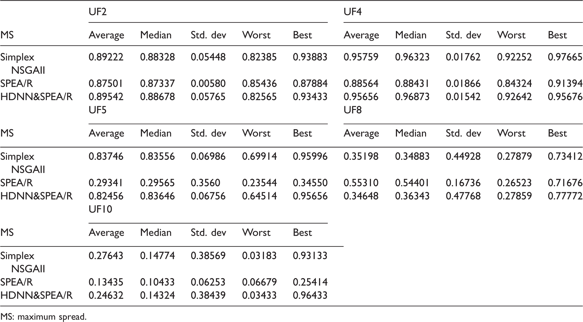
MS: maximum spread.
Similarly, parameters SP and MS in Tables 5 and 6 also show that HDNN&SPEA/R algorithm is the most dominant. Pareto optimal solution of HDNN&SPEA/R on each benchmark is also compared with the standard Pareto front set and the result of Simplex NSGAII algorithm as described in Figures 6 and 7.
Simulation results test benchmark functions
The resulting Pareto front is shown in Figures 6 and 7.
In this regard, Figures 6 and 7 show the comparison between the predicted results of HDNN&SPEA/R algorithms with the result of Simplex NSGAII algorithm being similar, but in terms of coverage, HDNN&SPEA/R algorithm is somewhat more outstanding. The results of both algorithms closely follow the results of benchmarking as shown in Figures 6 and 7. Therefore, it can be said that the proposed hybrid technique of HDNN&SPEA/R in this article has been successfully implemented.
The numerical results demonstrate that HDNN&SPEA/R is proposed to have better performance for benchmarking functions with two objectives related to convergence and coverage compared to SPEA/R algorithms. For some tri-objective benchmark functions, the proposed algorithm shows high convergence; it has high coverage. Thus, we could say the key advantages of the proposed HDNN&SPEA/R algorithm compared to SPEA/R and Simplex NSGAII algorithm are high convergence and coverage characteristics.
Simulation results test optimization of the Powertrain Mount System Stiffness Parameter
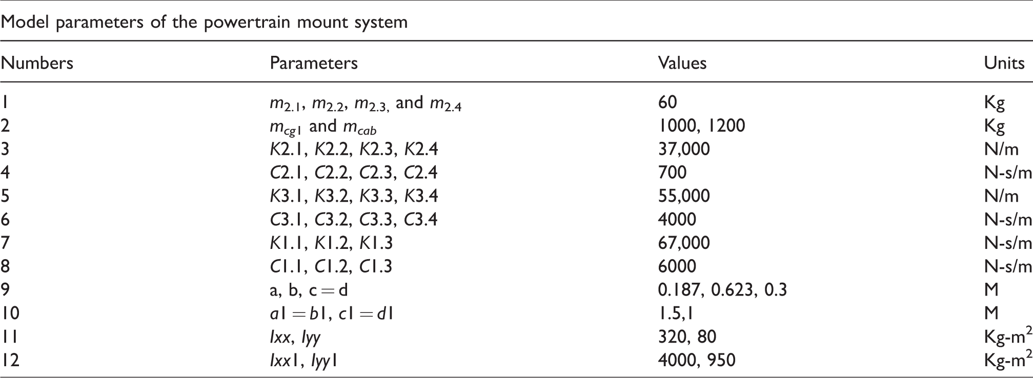
When the vehicle moves there are many factors that cause the vibration, the factors can be told: the internal force in the car; external forces appear in the process of using acceleration, braking, and revolving; exterior conditions such as wind and storm; and boring face street. Among the other factors is the bumpy side of the road which causes oscillation of the vehicle. To simulate the most general calculation, we use the road surface profile as a random function as in Figure 8 and simulated parameters as shown in Table 7.
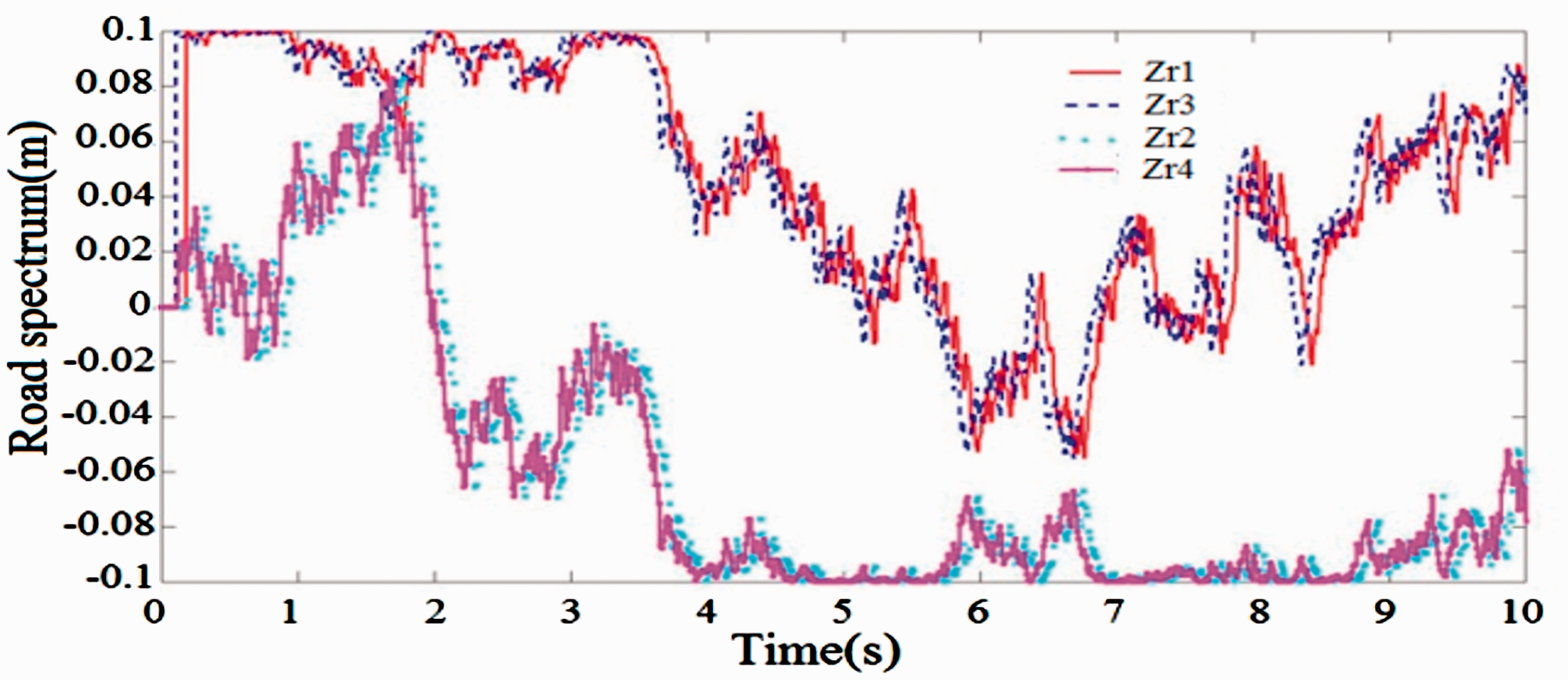
Road surface profiles.
Model parameters of the powertrain mount system.
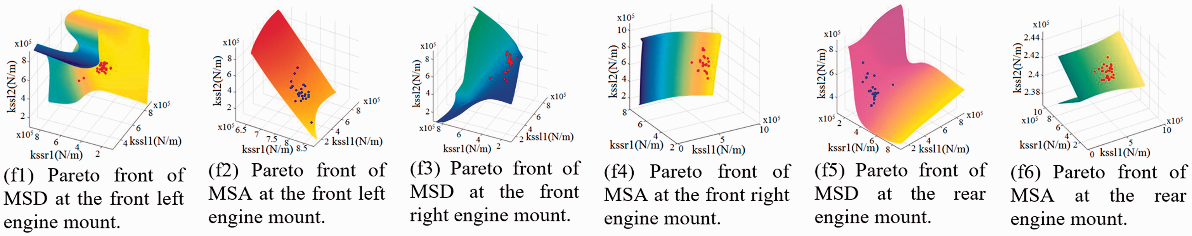
Through Matlab software and SPEA/R and HDNN&SPEA/R algorithms for simulation calculation to find Pareto front optimal set simultaneously of six functions of acceleration and displacement according to the stiffnesses of the front left, front right, and rear engine mount (K1.1, K1.2, and K1.3) value as shown in Figures 9 and 10 (Figures 9 and 10 shows the results in the form of 4 D via the isosurfaces function in Matlab).
Global Pareto front set of six-objective optimization functions with SPEA/R.
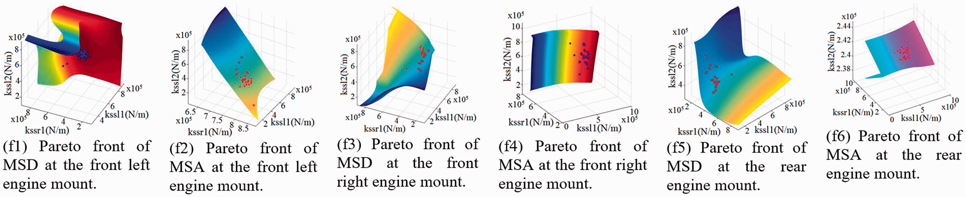
Global Pareto front set of six-optimization objective with HDNN&SPEA/R.
In order for a more intuitive look, the analytical results are presented in statistical form in the Tables 8 to 11.
Results for IGD of Powertrain mount system.
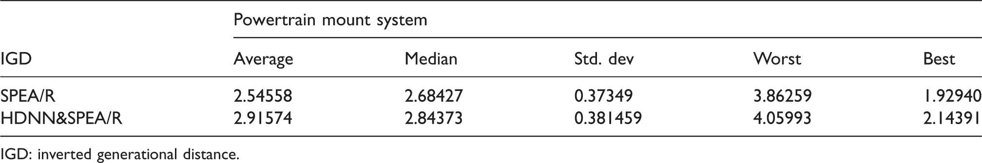
IGD: inverted generational distance.
Results for SP of Powertrain mount system.
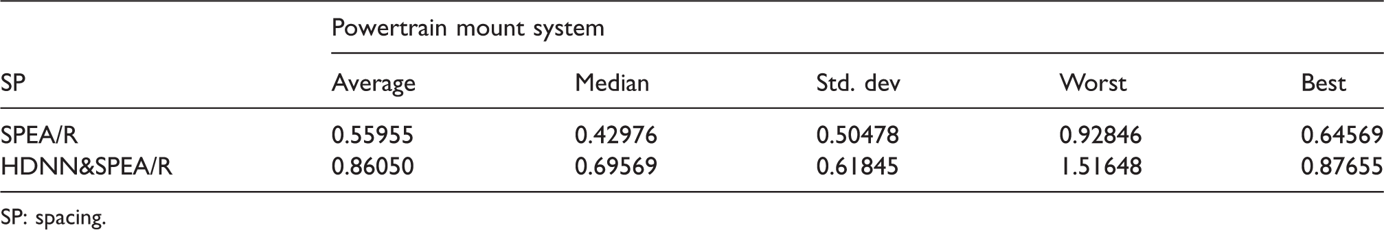
SP: spacing.
Results for MS of Powertrain mount system.
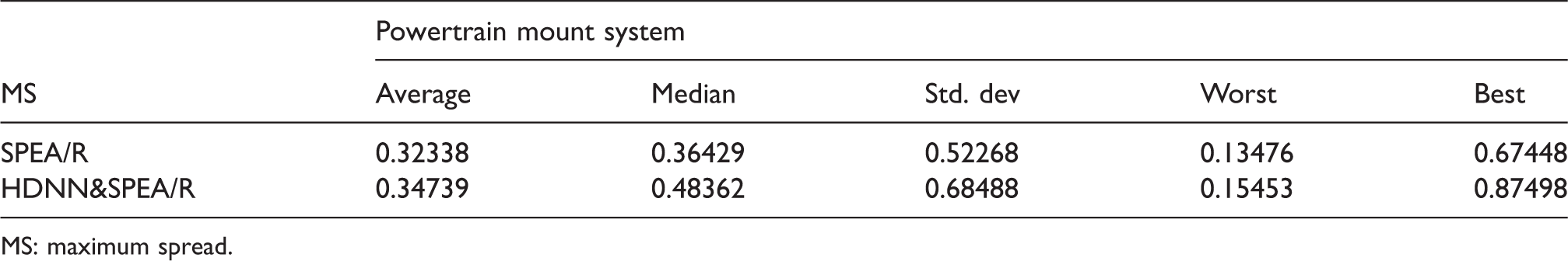
MS: maximum spread.
Results for time analysis compare of Powertrain mount system.
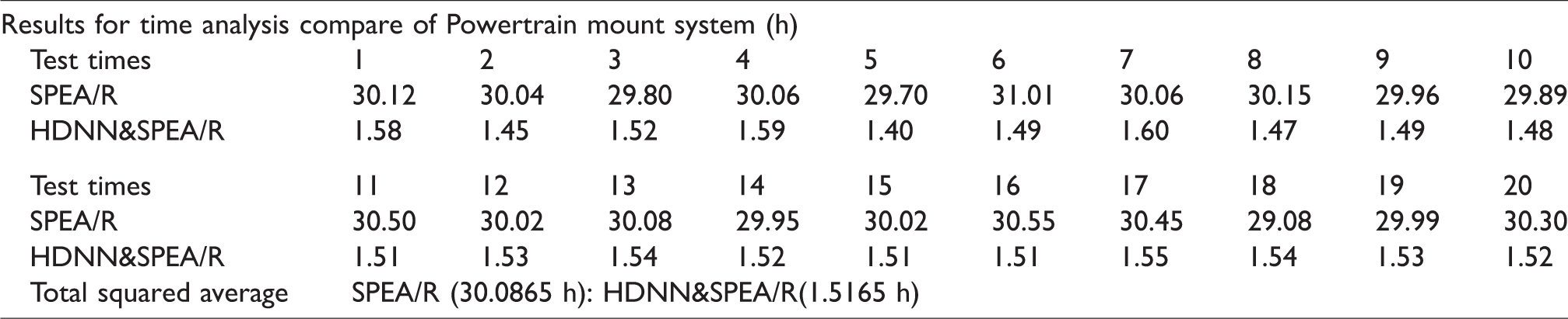
It is known that the result of multi-objective optimization will be a set of unaffected optimization points, called Pareto sets. These points provide a series of parameters for the designer to select the optimal point depending on his design conditions. There are always conflicting objective functions in the vehicle design that improving a function can adversely affect other functions. In this article, multi-objective optimization for all six target functions is done simultaneously. With the two results obtained from the two algorithms shown in Figures 9 and 10, we see Pareto front optimal set of two algorithms found relatively similar. But HDNN&SPEA/R algorithm has very fast computation time compared to SPEA/R algorithm. Therefore, through tests comparing two algorithms, HDNN&SPEA/R algorithms have proven superiority over SPEA/R algorithm because the time of calculation is extremely small, and the accuracy is completely reliable. That is, the optimal calculation time of HDNN&SPEA/R is much less than the SPEA/R algorithm. The results of the proposed HDNN&SPEA/R were in almost all cases better than SPEA/R.
Conclusion
This article has published a new combination method between SPEA/R, DNN, and GA. So ANNs with many hidden layers are trained with intelligent deep learning algorithms; it has created a deep learning network to realize the optimal problem simultaneously of many objects in the technology. This method is most effective and highly practical because: firstly, it offers a way of deep learning of the network with a much smaller number of standard samples than previous deep-learning networking methods announced. For test cases optimization of the Powertrain Mount System Stiffness Parameter, we only need a standard set of 15 samples to train DNNs. It is this combination of training that the actual number of samples generated for the training process is 15x(Iter_max) = 15,000 samples. While training with the old method is extremely difficult to collect a large number of samples. Secondly, for test cases optimization of the Powertrain Mount System Stiffness Parameter, the time for multi-objective optimal analysis of HDNN&SPEA/R hybrid methods is only 1.5 h, while using SPEA/R algorithm takes 30 h.
Footnotes
Declaration of conflicting interests
The author(s) declared no potential conflicts of interest with respect to the research, authorship, and/or publication of this article.
Funding
The author(s) disclosed receipt of the following financial support for the research, authorship, and/or publication of this article: This work was supported by the National Natural Science Foundation of China (51875096, 51275082).