Sage Journals: Discover world-class research

Abstract

In the absence of a priori knowledge, manual feature selection is too blind to find the sensitive features which can effectively classify the different fault features. And it is difficult to obtain a large number of typical fault samples in practice to train the intelligent classifier. A novel intelligent fault diagnosis method based on feature selection and deep learning is proposed for rotating machine mechanical in the paper. In this method, the deep neural network is not only used for feature extraction but also for fault diagnosis. First, the deep neural network 1 is used to extract feature from the spectral signal of the original signal. In addition, the original vibration signal is decomposed to a series of intrinsic mode function components by empirical mode decomposition, and the statistical features of each intrinsic mode function component are extracted by the deep neural network 2 in time domain and frequency domain. Second, the extraction features of the original signal spectrum and the extraction features of each intrinsic mode function component are evaluated, respectively. After features evaluation, the selected sensitive features are combined together to construct a joint feature. Finally, the joint feature is put into the deep neural network 3 to realize the automatic recognition of different fault states of rotating machinery. The experimental results show that the method proposed in this paper which integrated time-domain, frequency-domain statistical characteristics, empirical mode decomposition, feature selection, and deep learning methods can obtain the fault information in detail and can select sensitive features from a large number of fault features. The method can reduce the network size, improve the mechanical fault diagnosis classification accuracy, and has strong robustness.

Keywords

Intelligent fault diagnosis empirical mode decomposition feature selection denoising auto-encoder deep learning

Introduction

Rotating machinery is one of the most common mechanical equipment and plays an important role in industrial production.¹ In order to improve productivity and product quality, the mechanical equipment must be in trouble-free operation. However, mechanical equipment often operates in complex working environment and mechanical equipment components often fail. Once an equipment component fails, which will produces a chain reaction, mechanical failure of equipment will occur. Fault diagnosis technology is an important technical means to avoid mechanical failure, which is of great practical significance to the normal operation of the mechanical equipment.^2,3

During the past decades, researchers have given considerable attention to rotating machinery fault diagnosis, and many intelligent fault diagnosis approaches have been proposed in literature.^4–8 Samanta⁴ extracted time-domain features and employed three optimized neural networks to detect pump faults. Samanta and Nataraj⁵ utilized time-domain features to characterize the bearing health conditions and employed artificial neural networks and support vector machine (SVM) to diagnose faults of bearings. Tran et al.⁶ calculated features from thermal imaging based on bi-dimensional empirical mode decomposition (EMD), and then input selected features into relevance vector machine (RVM) for fault classification. Widodo et al.⁷ calculated statistical features from the measured signals and carried out RVM and SVM to diagnose the bearing faults. Bin et al.⁸ utilized wavelet packets-EMD to extract fault feature. Deep neural network (DNN) is a kind of burgeoning intelligent classifier in recent years.^9–16 Wang et al.⁹ studied a novel convolutional neural network-based fault recognition method via image fusion of multi-vibration signals. Huang et al.¹⁰ proposed a novel method called deep decoupling convolutional neural network for intelligent compound fault diagnosis. Kane and Andhare¹¹ used artificial intelligence techniques to identify gearbox condition in the above environment by using psychoacoustic features to replace human hearing. Chen et al.¹² studied fault diagnosis of wind turbine gearbox based on wavelet neural network. Jia et al.¹³ used DNN to extract fault feature from the massive data. Gan et al.¹⁴ constructed a hierarchical diagnosis network based on DNN and then applied it in the fault pattern recognition of rolling element bearings. DNN has been applied in the field of fault diagnosis of mechanical equipment.^15,16 The DNN is first pretrained by an unsupervised layer-by-layer learning and then fine-tuned with the back propagation (BP) algorithm, where the unsupervised process helps the fault characteristic mining and the supervised process contributes to construct the discriminative fault characteristics for classification. DNN pretraining uses a large number of unlabeled samples for unsupervised training. Only a small number of labeled samples need to be entered in the fine-tuning stage to fine-tune the parameters of the DNN. So the DNN solves the problem that it is difficult to obtain a large number of typical fault samples in reality.

For realizing a large number of typical fault sample diagnoses, Silva et al.¹⁷ proposed feature selection method based on the several feature selection methods. Lei et al.¹⁸ presented a fault diagnosis method of rotating machinery based on a new clustering algorithm using a compensation distance evaluation technique, and the diagnosis result demonstrated the superior effectiveness and practicability of the algorithm. Yang and co-workers^19,20 applied the feature evaluation technology to the equipment intelligent fault diagnosis and the result proved the validity of feature selection. Sawhney and Jeyasurya²¹ combined with two kinds of feature selection techniques and the former neural network for power system stability assessment, the experimental test has achieved effective results.

The common intelligent fault diagnosis methods generally include two main steps: fault feature extracting using signal processing methods and fault classification using classifiers. At the same time the common intelligent fault diagnosis methods have two obvious deficiencies: (1) the extracted features not only contain a large number of fault features, but also contain some redundant features. These redundant features will not contribute to the classification and even reduce the accuracy of classification. Thus, it is necessary to select the features before classification so as to screen out the sensitive features, thus reducing the network size, improving the accuracy of the classification of the classifier. (2) Supervised classifiers such as SVM^22–24 and back propagation neural network (BPNN)^25,26 require a large amount of labeled data to be trained to adjust the parameters. But it is difficult to obtain a large number of typical fault samples in reality. Therefore, an unsupervised classifier with high accuracy and robustness or a classifier that only needs a small amount of labeled data to train is needed.

This paper proposes a novel intelligent diagnosis method to overcome the two deficiencies of the common intelligent fault diagnosis methods in fault diagnosis of rotating machinery. The novel intelligent diagnosis method combines feature selection and DNN method. The feature selection method is based on the distance between the features to select the sensitive features. Its selection principle is that the distance between the same classes is the smallest and the distance between the different classes is the largest. Through the feature selection, it can select the sensitive features which are good at recognizing the different fault states. The nonsensitive features to the classification accuracy are removed. Therefore, the scale of the neural network is reduced and the classification accuracy improved. First, the original features are preselected, and then the original strong feature technology is used to select the final strong feature. The comparison results show that the proposed method not only can improve the accuracy but also save running time.

The rest of this paper is organized as follows: the next section briefly introduces the feature extraction method and the burgeoning feature extraction method based on the DNN. “Rotating machinery fault diagnosis process of the proposed method” section presents the proposed method for the rotating machinery fault diagnosis and its process. “Fault diagnosis using the proposed method” section describes two diagnosis cases of rolling element bearings and gearboxes to validate the proposed method, respectively. Conclusions are drawn in the final section.

Feature extraction, feature selection, and state recognition

Fault diagnosis is essentially a pattern recognition problem, which includes three parts: signal acquisition, feature extraction, and state recognition. Signal acquisition is the premise of fault diagnosis, feature extraction is the key of fault diagnosis, and state recognition is the core of fault diagnosis.^27–29 Statistical features in the time domain include maximum value, absolute mean, peak to peak value, root mean square (RMS), skewness, kurtosis, shape factor, crest factor, impulse factor, and margin factor. The frequency spectrum of the vibration signal indicates the amplitude change of vibration signal with frequency distribution. When the frequency components of the signal increase or decrease, the energy distribution of the spectrum is shown to be dispersed or concentrated. The characteristic parameters provide effective information of fault diagnosis for rotating machinery through spectrum analysis. Common statistical features are the center gravity of frequency domain and frequency domain variance. Fast Fourier transform (FFT) frequency spectrum analysis method is generally used to select the characteristic frequency for state monitoring and fault diagnosis of rotating machinery.

Feature extraction based on DNN with EMD

In 2006, Hinton et al.³⁰ discussed the deep learning theory. Deep learning is designed to simulate the learning process of the brain, combined with a large number of training data to study the features of the data. Deep learning neural network can not only extract features but also recognize different states. In the process of condition monitoring and fault diagnosis of rotating machinery, there are still a lot of nonlinear and nonstationary signals. EMD is an effective nonstationary and nonlinear signal processing technique based on the local characteristic time scale of the signal.

This paper proposed a novel feature extraction method based on DNN with EMD. The DNN is composed of a plurality of denoising automatic encoders (DAEs). Figure 1 shows the structure of the DAE. DAE is the three layers of unsupervised neural network, which is divided into two parts: encoding network and decoding network. The input and output layers in denoising auto-encoder have the same number of nodes. High dimension of input data can be reduced by encoding network and reconstructing the coding vector of low-dimensional space to the original input data. Coding network introduces the noise with some statistical characteristics into the sample data, and then codes the sample; the decoding network is estimated in the original form of the sample without noise interference according to the data subject to noise interference. So that DAE can learn from the noisy samples to extract more robust features and reduce the sensitivity of DAE to small random perturbations. The DAE principle is similar to the human body’s sensory system, such as observing objects. DAE can effectively reduce the influence of random factors on the extraction of health information and improve the robustness of the feature expression by adding noise to the coding and reconstruction. Between the coding layer and the decoding layer is the hidden layer; it also called the “code word layer,” which is the core of the whole DAE. The low-dimensional coding vector of the hidden layer can reflect the nature of the high-dimensional input data. In other words, low-dimensional coding is a characteristic expression of high-dimensional inputs from another aspect.

Figure 1.

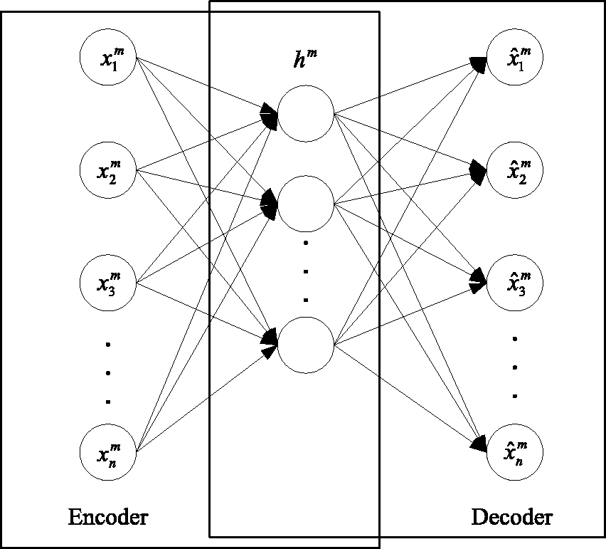
Architectural graph of the denoising auto-encoder.

At the same time, the vibration signals of rotating machinery are decomposed by EMD, and the statistical characteristics of the time domain and frequency domain of the front eight intrinsic mode function (IMF) components are obtained. The time-domain feature parameters are the maximum value, absolute mean and peak to peak, RMS, skewness, kurtosis, shape factor, crest factor, impulse factor, and margin factor; frequency-domain parameters are the center gravity of frequency domain and frequency domain variance.

Feature selection

The paper studied the feature selection method based on the distance between the features to select the sensitive features. The feature selection principle is that the distance between the same classes is the smallest and the distance between the different classes is the largest. Features that are consistent with the principles are considered sensitive features. That is to say, smaller the distance between the same classes and larger the distance between the different classes are more sensitive to this feature. The steps of the selection method are as follows:

Step 1: Calculate the inner distance of the i feature of the j class

\begin{array}{l} d_{i, j} = \frac{1}{N (N - 1)} \sum_{m, n = 1}^{N} | p_{i, j} (m) - p_{i, j} (n) | \\ m, n = 1, 2, \dots, N, m \neq n, i = 1, 2, \dots, K \\ j = 1, 2, \dots, M \end{array}

(1)

where N indicates the number of samples; K represents the number of features; M represents the number of classes;

p_{i, j} (m)

and

p_{i, j} (n)

, respectively, are the i feature of the m sample of the j class and i feature of the n sample of the j class.

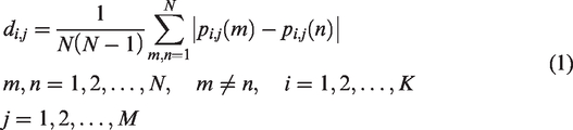
Calculate the average value of the inner distance of the j class of the i feature

D_{i} = \frac{1}{M} \sum_{j = 1}^{N} d_{i, j}

(2)

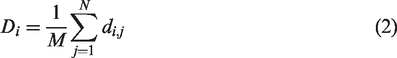
Step 2: Calculate the average value of the i feature of the N sample of the j class

q_{i, j} = \frac{1}{N} \sum_{n = 1}^{N} p_{i, j} (n)

(3)

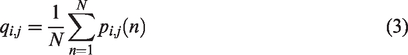
Then, calculate the average value of the inter-distance of the M class of the i feature

\begin{array}{l} D_{i}^{'} = \frac{1}{M (M - 1)} \sum_{u, w = 1}^{M} | q_{i, u} - q_{i, w} | \\ u, w = 1, 2, \dots, M, u \neq w \end{array}

(4)

where

q_{i, u}

and

q_{i, w}

, respectively, are the average value of the i feature of the N sample of the u class and i feature of the N sample of the w class.

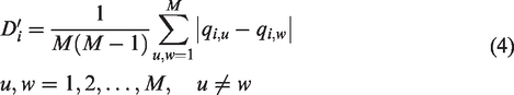
Step 3: Calculate the evaluation factor of the i feature

α_{i} = D_{i}^{'} / D_{i}

(5)

The size of $α_{i}$ reflects the degree of difficulty in classifying the M class with the i features. Greater the $α_{i}$ is, more sensitive the i feature is, easier to classify the M classes.

Step 4: Sort the features from large to small in accordance with the value of $α_{i}$ , then increase the number of features one by one, put the selected features into the SVMs for training and testing. If the number of features exhibits a continuous increase of 5 and there is no improvement in classification accuracy, then stop increasing the number of features; at this time, the selected features are the most sensitive features.

State recognition

In this paper, DNN is used as the state recognition classifier. DNN has a strong ability of nonlinear expression and good ability to judge. When building a model, there is no need to train the model with a large number of labeled data. This paper uses the stack denoising auto-encoder neural network. The following focuses on the working principle of the denoising auto-encoder and the pretraining and fine-tuning of DNN.

DAE working principle

The structure of the denoising auto-encoder is shown in Figure 1. The following focuses on the working principle of the denoising auto-encoder. As shown in Figure 2, given a label free training sample set ${x^{m^{'}}}_{m = 1}^{M}$ , in the coding network put the noise qD which has the regular statistical properties into the training sample data $x^{m}$ . The coding network transforms each training sample $z^{m}$ to the coding vector $h^{m}$ by the coding function $f_{θ}$

h^{m} = f_{θ} (z^{m}) = s_{f} (w z^{m} + b)

(6)

where

s_{f}

is the activation function of the coded network;

θ

is the parameter set for the coded network, and

θ = {w, b}

; where

w

and

b

, respectively, are the connection weights and bias parameters of the coding network.

Figure 2.

Schematic of a denoising auto-encoder.

The decoding network transforms each $h^{m}$ to the decoding vector $y^{m}$ by the decoding function $g_{θ^{'}}$

y^{m} = g_{θ^{'}} (h^{m}) = s_{g} (w^{'} h^{m} + d)

(7)

where

s_{g}

is the activation function of the decoded network;

θ^{'}

is the parameter set for the decoded network, and

θ^{'} = {w^{'}, d}

, where

w^{'}

and

d

, respectively, are the connection weights and bias parameters of the decoding network.

DAE completes the training of the whole network by minimizing the reconstruction error between $x^{m}$ and $y^{m}$

L (x^{m}, y^{m}) = \frac{1}{M} {‖ x^{m} - y^{m} ‖}^{2}

(8)

Pretraining and fine-tuning of DNN

DNN is first trained by the unsupervised method, which can help the DNN to capture the fault characteristics of the input signal effectively. Then, DNN is adjusted by the supervised learning method to optimize the expression of DNN on the fault characteristics. This paper uses denoising auto-encoder as a non-unsupervised algorithm for pretraining and uses the BP algorithm as the supervised algorithm for fine-tuning stage.

Pretraining is an unsupervised learning from bottom to top. First, the first layer is trained with the training sample data, and the connection weights and the bias parameters of the first layer are obtained. By the principle of denoising auto-encoder, DAE model can learn the structure of the data itself and identify the characteristics of the input. The output of the first layer is used as the input of the second layer. Train the second layer to get the connection weights and bias parameters of the second layer, and so on. The final features are reconstructed based on the learning of multiple layers.

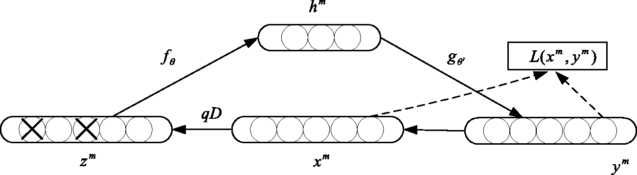
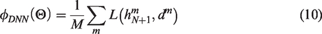
Fine-tuning is supervised learning from top to bottom. With the labeled training data, the error transports from top to bottom to fine-tune the DNN. This process is a supervised training process. Specific as shown in Figure 3, this method uses the BP algorithm to fine-tune the DNN parameters. The output of DNN is expressed as

h_{N + 1}^{m} = f_{θ_{N + 1}} (h_{Nm})

(9)

where

θ_{N + 1}

is the parameter of the output layer.

Figure 3.

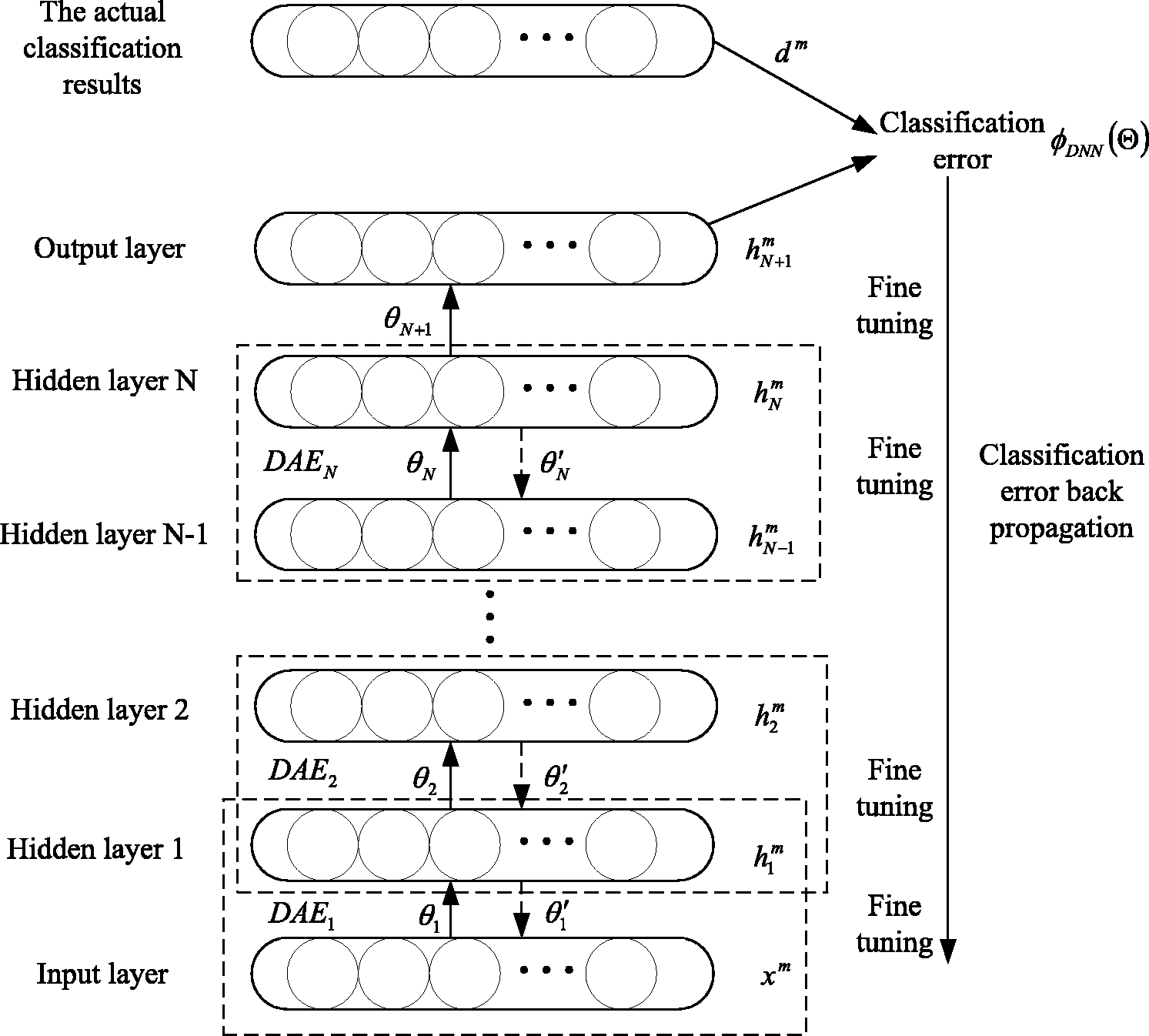
Pretraining and fine-tuning of the DNN.

Assume that $x^{m}$ of the health condition type is $d^{m}$ , DNN is fine-tuned by minimizing the $ϕ_{DNN} (Θ)$

ϕ_{DNN} (Θ) = \frac{1}{M} \sum_{m} L (h_{N + 1}^{m}, d^{m})

(10)

where

Θ

is the parameter set of DNN, and

Θ = {θ_{1}, θ_{2}, \dots, θ_{N + 1}}

.□

Rotating machinery fault diagnosis process of the proposed method

The proposed method, respectively, extracts fault features of vibration signal of rotating machinery from two angles: Transform the vibration signal with the FFT, and then put the frequency spectrum of the signal into the DNN1 to extract features; decompose the vibration signal with the EMD method, then calculate each IMF component’s time-domain and frequency-domain statistical features, put the statistical features into the DNN2 to extract further features. Estimate the two extracted features, respectively, and select the sensitive features. Put the sensitive features into the DNN3 to recognize and diagnosis of fault state. The DNN1 and the DNN2 mainly use the denoising auto-encoder to extract features to reduce the DNN3’s size. The DNN3 mainly achieves classification function. The flow chart is shown in Figure 4 Rolling bearing test platform of West University is shown in Figure 5.

Figure 4.

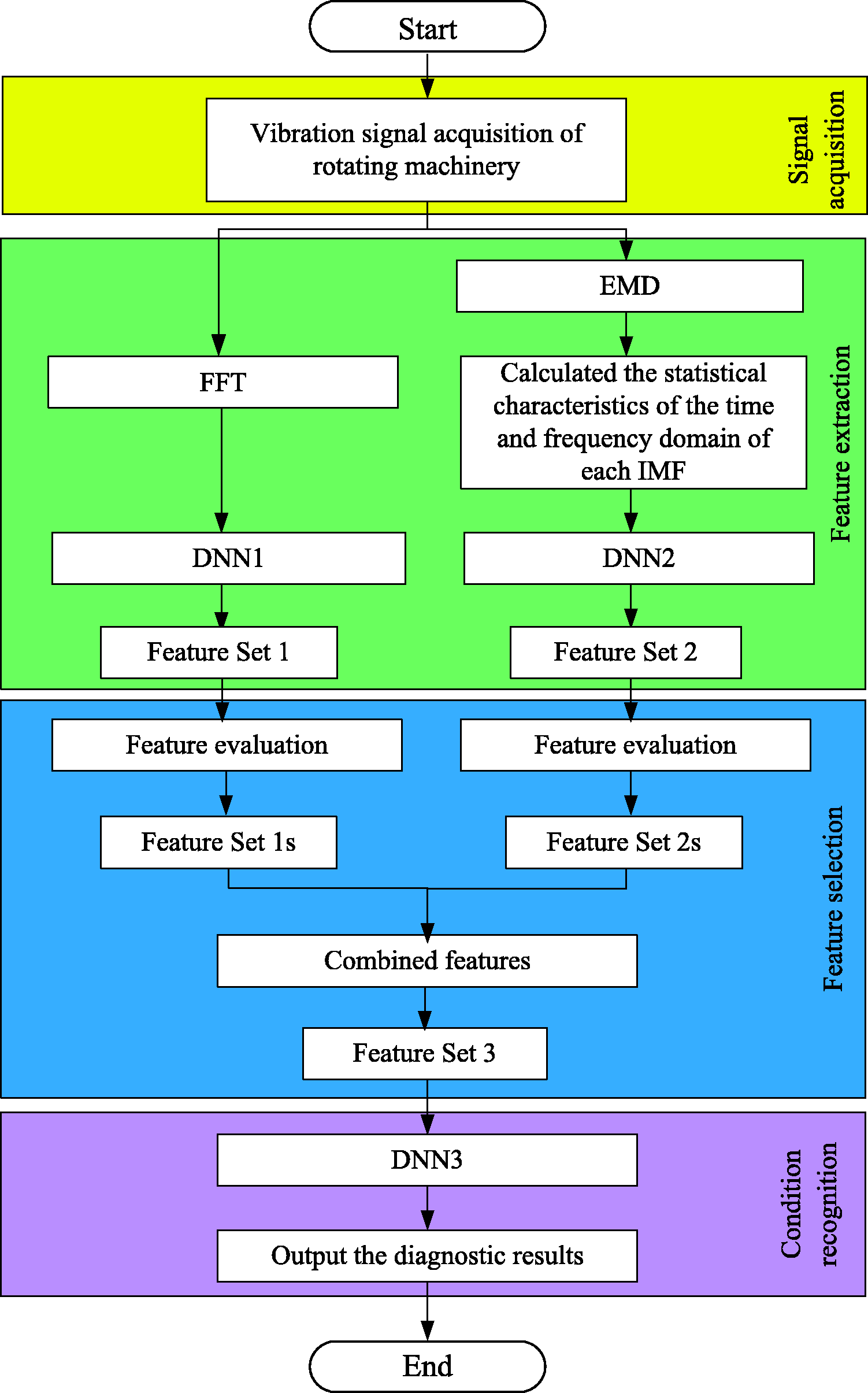
Flow chart of rotating machinery fault diagnosis based on feature selection and deep learning. DNN: deep neural network; EMD: empirical mode decomposition; FFT: Fast Fourier transform

Figure 5.

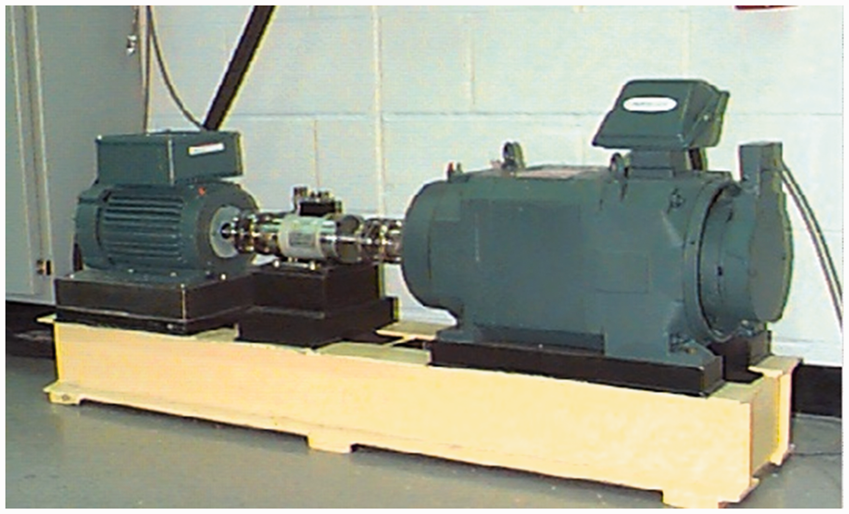
Rolling bearing test platform of West University.

The specific steps are as follows:

Step 1. Signal acquisition: Get the vibration signal of rotating machinery under different conditions

Step 2. Feature extraction: Transform the vibration signal in each state with the FFT and then put the obtained spectral signal into the DNN1 to extract features. The extracted features are called feature set 1. Decompose each state of the vibration signal with the EMD method to get a number of IMF components. Calculate the statistical features of the time domain and frequency domain of each IMF component. Then put the statistical features into the DNN2 to extract further features. The further extracted features are called feature set 2.

Step 3. Feature selection: Feature selection based on distance estimation algorithm is used to feature set 1 and feature set 2, respectively. Then pick out the sensitive features to form the feature set 3.

Step 4. Condition recognition: Put the selected sensitive Feature Set 3 into the DNN3 to intelligent fault diagnosis of rotating machinery.

Fault diagnosis using the proposed method

Rolling element bearings and gears are the key components in rotating machinery.^31,32 The health conditions of these components often affect the performance, reliability, and service life of the machinery. Whereas due to tough working environment, these components easily suffer from different kinds of damage leading to breakdowns and heavy economic losses.^33,34 In this section, two diagnosis cases of rolling element bearings and gearboxes are used to validate the proposed method, respectively.

Case 1: Fault diagnosis of rolling element bearings

Data description

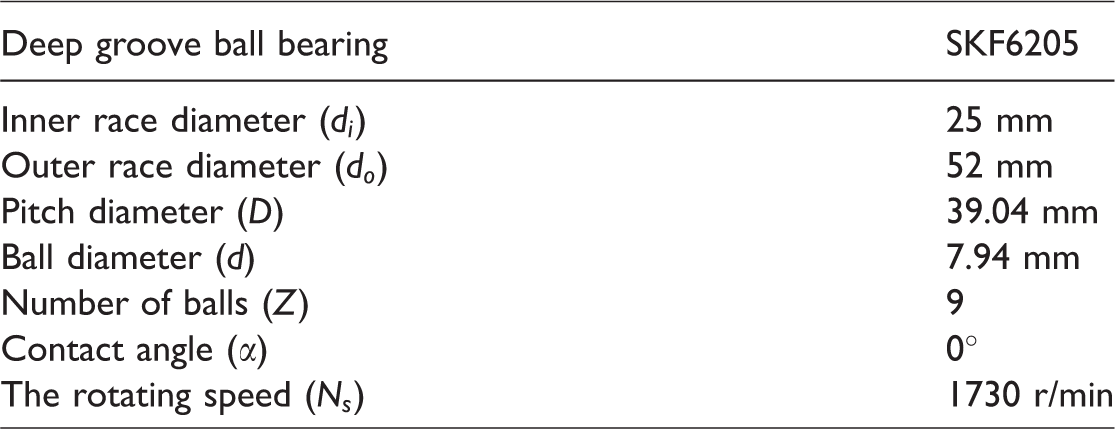
The experimental parameters are provided in Table 1. And the ball pass frequency on outer race (BPFO) and the ball pass frequency on inner race (BPFI) are calculated with shaft speed $(BPFO) = \frac{Z N_{s}}{2 \times 60} (1 - \frac{d}{D} \cos α)$ =103.36 Hz; $(BPFI) = \frac{Z N_{s}}{2 \times 60} (1 + \frac{d}{D} \cos α)$ =156.14 Hz.

Table 1.

Experimental parameters.

Deep groove ball bearing	SKF6205
Inner race diameter ( $d_{i}$ )	25 mm
Outer race diameter ( $d_{o}$ )	52 mm
Pitch diameter ( $D$ )	39.04 mm
Ball diameter ( $d$ )	7.94 mm
Number of balls ( $Z$ )	9
Contact angle ( $α$ )	0°
The rotating speed ( $N_{s}$ )	1730 r/min

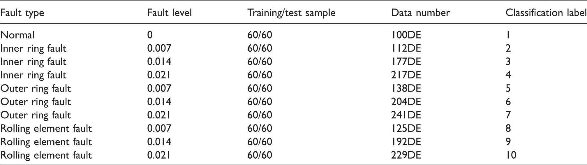
The bearing data used here are provided by the Case Western Reserve University.³⁵ The data were collected from a motor driving mechanical system under 3 HP load loads with the sampling frequency of 48 kHz. The bearing dataset was obtained from the experimental system: (1) under normal condition, (2) with outer race fault, (3) with inner race fault, and (4) with roller fault. The faults were introduced into the drive end bearing of the motor with fault diameters of 0.18, 0.36, and 0.54 mm, respectively. So this test has 10 different working conditions. For each working condition, we divide the collected data into 120 samples and each sample has 4000 sample points. For each working condition, we randomly select 60 groups of samples as the training samples, and use the remaining 60 groups of samples as test samples, as shown in Table 2.

Table 2.

The detail lists of the test and training samples.

Fault type	Fault level	Training/test sample	Data number	Classification label
Normal	0	60/60	100DE	1
Inner ring fault	0.007	60/60	112DE	2
Inner ring fault	0.014	60/60	177DE	3
Inner ring fault	0.021	60/60	217DE	4
Outer ring fault	0.007	60/60	138DE	5
Outer ring fault	0.014	60/60	204DE	6
Outer ring fault	0.021	60/60	241DE	7
Rolling element fault	0.007	60/60	125DE	8
Rolling element fault	0.014	60/60	192DE	9
Rolling element fault	0.021	60/60	229DE	10

Experimental configurations and diagnosis results

The DNN input layer is determined by the number of input feature vectors, and the output layer is determined by the classification label. Because the time-domain sampling number of each sample is 4000 points, the spectrum of the Fourier transform is symmetrical, so the first 2000 sampling points of the spectrum are taken as the input vector of DNN1. In this paper, the network structure of DNN1 is set to 2000–500–300–200–10. Decompose the selected samples with the EMD method. Because the main fault information is concentrated in the front few IMF components, so this paper selected the front eight IMF components. Calculate the time-domain and frequency-domain statistical features of each IMF component (8 × 12 = 96), and put them into the DNN2 as the input feature vectors. The network structure of DNN2 is set to 96–60–30–10. The 200 features which are extracted by the DNN1 third hidden layer are called feature set 1; the 30 features which are extracted by the DNN2 second hidden layer are called feature set 2.

Then we evaluate the feature set 1 and the feature set 2 with the distance estimation algorithm. The evaluation factor of each feature of feature set 1 and feature set 2 is shown in Figure 6. Sort the features from large to small in accordance with the value of $α_{i}$ , then increase the number of features one by one, put the selected features into a classifier to determine the best sensitive features. Figure 6 shows the relationship between the classification accuracy and the number of input features of the feature set 1 and feature set 2. The trend of the curve can be seen from Figure 6 and the front increase features have a strong sensitivity. So the classification accuracy is improved with the increase of the number of features. But when the number of features of the input network increased to a certain degree, the classification accuracy rate began to decline. Due to the subsequent increase features are insensitive to the classification of different fault states. With the increase of the number of features, the difference between different fault states becomes more and more fuzzy. As a result, the accuracy of classification is decreased because of the increase of the feature.

Figure 6.

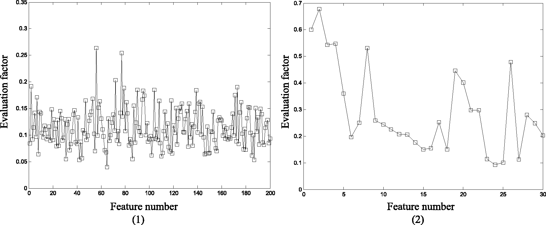
(a) Evaluation factors of 200 features of feature set 1 and (b) evaluation factors of 30 features of feature set 2.

From Figure 7, we know the classification accuracy is the highest when the input is the front 50 sensitive features and the front 10 sensitive features. So we choose the 50 sensitive features as the feature set 1s and the 10 sensitive features as the feature set 2s. Feature set 1s and feature set 2s constitute the joint feature which is called the feature set 3. Then put the feature set 3 into the DNN3 for classification. The network structure of DNN3 is set to 60–40–30–10. The feature set should be normalized before put into the DNN, because the classification accuracy can be improved and the calculation time can be reduced by normalizing. Put the different input feature sets into the DNN to obtain the classification accuracy, respectively. Repeat the test five times to get the average classification accuracy. The results are shown in Table 3.

Figure 7.

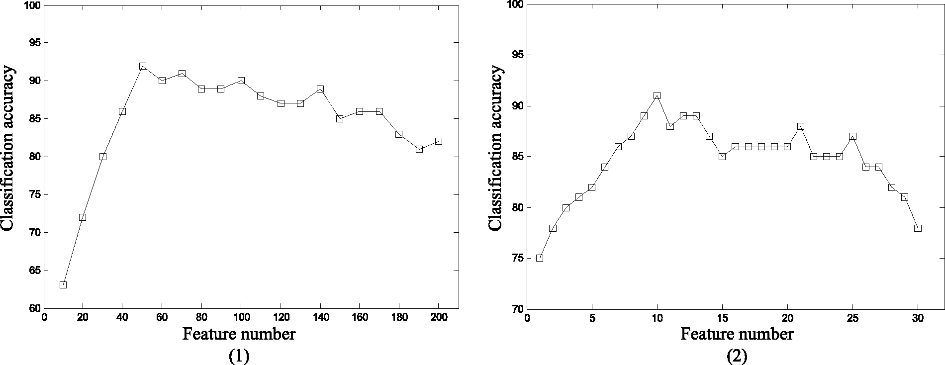
(a) The relationship between the classification accuracy and the number of input features of the feature set 1 and (b) the relationship between the classification accuracy and the number of input features of the feature set 2.

Table 3.

Fault diagnosis results of different input feature sets.

Input feature set	Classification accuracy (%)
Feature set 1	82.67
Feature set 2	78.00
Feature set 1s	92.33
Feature set 2s	89.17
Feature set 3	98.50

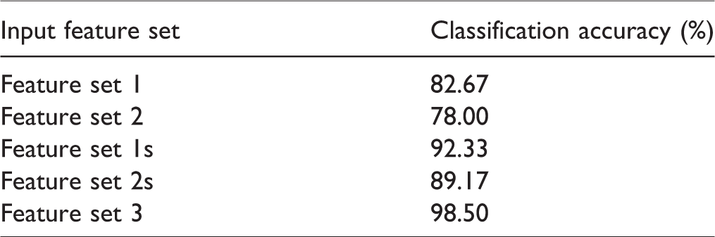
Based on the results in Table 3, it is found that the feature set 1 is classified by the DNN, and the accuracy is 82.67%. The feature set 2 is classified by the DNN, and the accuracy is 78%. The feature set 1s is classified by the DNN, and the accuracy is 92.33%. The feature set 2s is classified by the DNN, and the accuracy is 89.17%. Feature set 1 and feature set 2 not only contain a large number of fault features, but also contain a large number of redundant features. If they are directly put into the classifier, the classification process will be slow, and the classification accuracy will be reduced. Therefore, feature selection should be performed before classification so as to screen out the sensitive features, thus reducing the network size, improving the accuracy of the classification of the DNN. Feature set 1s and feature set 2s are fault features of rotating machinery vibration signals which are extracted from two angles, respectively. And different input feature sets usually show complementary classification characteristics. So this paper combines feature set 1s and feature set 2s to form the joint feature set 3. And then put the feature set 3 into the DNN3 classification, the accuracy is 98.5%. Compared with the feature set 2s and feature set 1s, the accuracy is improved.

Case 2: Fault diagnosis of gearboxes

Experiments and data description

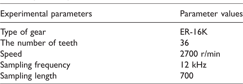
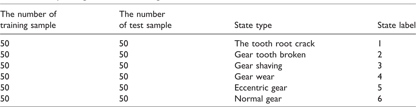
The gearbox data used here are provided by the multi-stage gear transmission system experimental bench which is shown in Figure 8. The test bench can simulate a variety of gearbox fault, such as gear wear, gear broken teeth, gear shaving, tooth root crack and eccentric gear, etc. Experimental parameters are shown in Table 4. Six operating states of the test gear are shown in Table 5. The original vibration signal is measured by using the acceleration sensor under six operating states of the test gear. And the time-domain signal and the frequency-domain signal of the original vibration are shown in Figure 9.

Figure 8.

Multi-stage gear transmission system experimental bench.

Table 4.

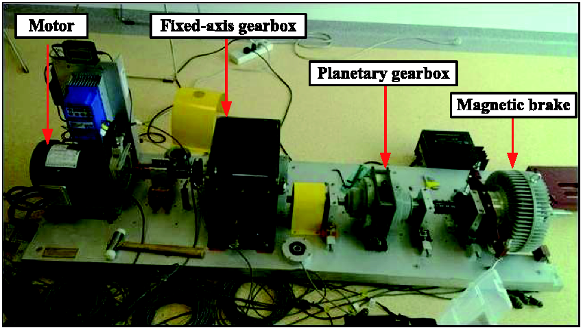
Experimental parameters of the multi-stage gear transmission system experimental bench.

Experimental parameters	Parameter values
Type of gear	ER-16K
The number of teeth	36
Speed	2700 r/min
Sampling frequency	12 kHz
Sampling length	700

Figure 9.

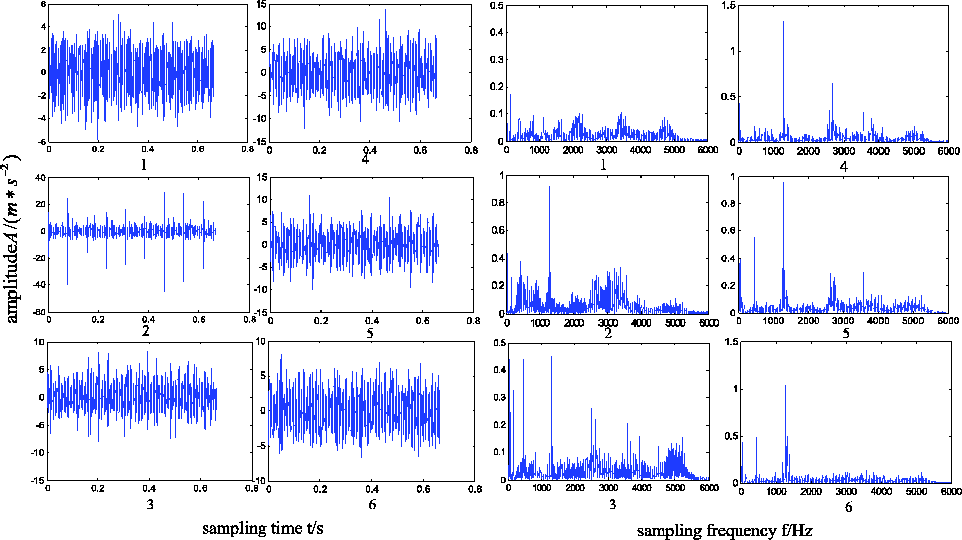
Time-domain waveform and frequency spectrum of the original vibration signal.

Table 5.

Six operating states of the test gear.

The number of training sample	The number of test sample	State type	State label
50	50	The tooth root crack	1
50	50	Gear tooth broken	2
50	50	Gear shaving	3
50	50	Gear wear	4
50	50	Eccentric gear	5
50	50	Normal gear	6

Experimental configurations and diagnosis results

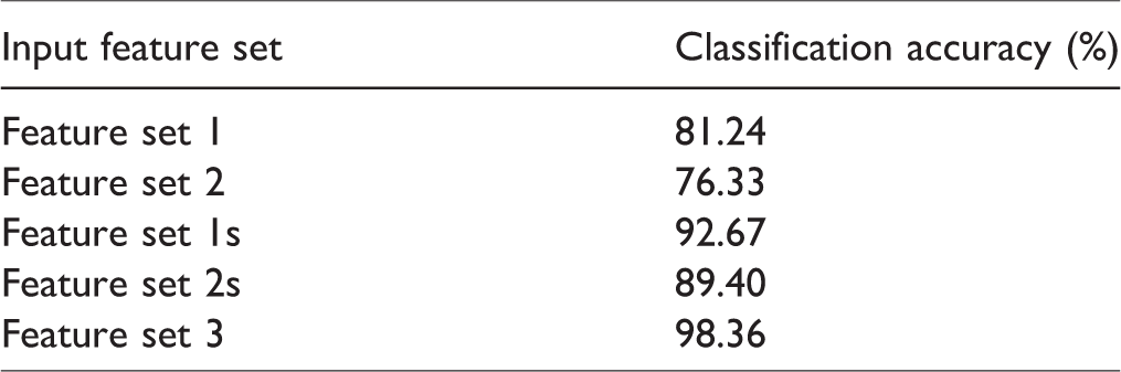
The DNN input layer is determined by the number of input feature vectors, and the output layer is determined by the classification label. As the original vibration signal spectrum has 350 points and the state label is 6, the network structure of DNN1 is set to 350–250–150–6. Decompose the selected samples with the EMD method and select the front eight IMF components. Calculate the time-domain and frequency-domain statistical features of each IMF component (8 × 12 = 96). And the network structure of DNN2 is set to 96–60–30–6. The 150 features which are extracted by the DNN1 second hidden layer are called feature set 1; the 30 features which are extracted by the DNN2 second hidden layer are called feature set 2. Evaluate the feature set 1 and the feature set 2 with the distance estimation algorithm. Then we choose the 42 sensitive features as the feature set 1s and the 11 sensitive features as the feature set 2s. Feature set 1s and feature set 2s constitute the joint feature which is called the feature set 3. Then put the feature set 3 into the DNN3 for classification. The network structure of DNN3 is set to 53–40–30–6. Put the different input feature sets into the DNN to obtain the classification accuracy, respectively. Repeat the test five times to get the average classification accuracy. The results are shown in Table 6.

Table 6.

Fault diagnosis results of different input feature sets.

Input feature set	Classification accuracy (%)
Feature set 1	81.24
Feature set 2	76.33
Feature set 1s	92.67
Feature set 2s	89.40
Feature set 3	98.36

In order to verify the superiority of the DNN, different classifiers are used to compare the classification accuracy. Put feature set 3 into BPNN and SVM, respectively, and the test was carried out for 15 times. The structure of BPNN is set to 53–40–30–10. SVM uses the radial basis kernel function, its kernel parameter and penalty factor are optimized by the particle swarm optimization algorithm. Calculate the average of the 15 test accuracy and the corresponding standard deviation, the result is shown in Table 7.

Table 7.

Fault diagnosis results of different classifiers.

Classifier type	Average accuracy (%)	Accuracy standard deviation
BPNN	83.167	17.333
SVM	91.667	6.625
DNN	96.333	2.225

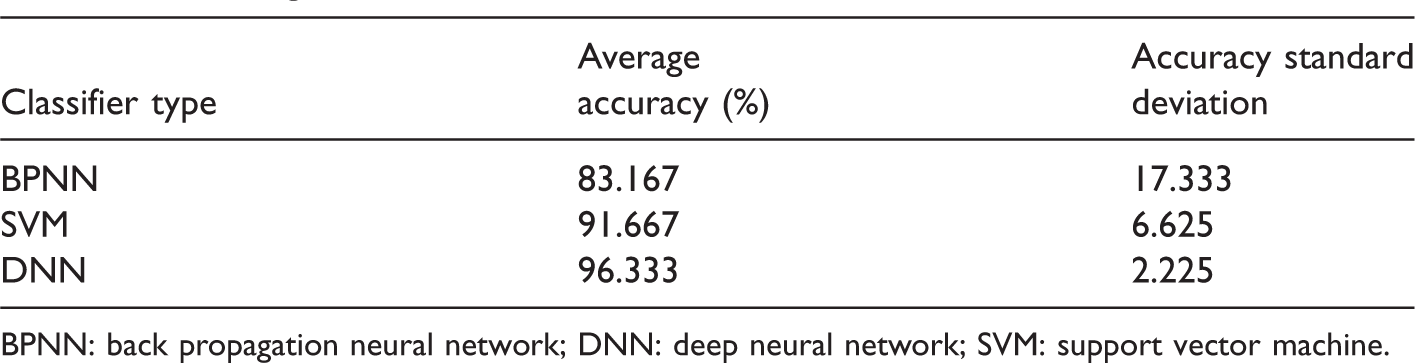
BPNN: back propagation neural network; DNN: deep neural network; SVM: support vector machine.

Compared with the three classifiers, the accuracy of the DNN is the highest, and the stability of the diagnosis is the best. The principle of BPNN is different from that of DNN. DNN trains the input feature vector layer upon layer. So the BPNN training errors are sometimes convergent, and sometimes fall into the local optimum, which leads to the accurate rate of diagnosis fluctuating violently. SVM classifier can be accurate and stable for the diagnosis. But SVM cannot reduce input feature vector dimension for further feature learning as DNN. Compared with DNN, SVM has worse generalization ability.

The SVM is a better method to realize the structural risk minimization principle, which provides a new way of thinking to solve the small sample size classification, nonlinear problem. The basic idea of SVM is to increase dimension and linearization: define the optimal linear hyper plane, and reduce the algorithm of finding the optimal linear hyper plane to a convex programming problem. Then, based on the Mercer kernel expansion law, the sample space is mapped to a high-dimensional and even infinite dimensional feature space by nonlinear mapping, so as to the linear learning machine can be used in the feature space to solve the problem of highly nonlinear classification and regression in the sample space. 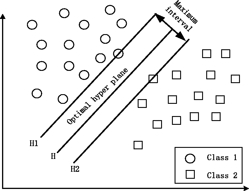Suppose a training set with m samples $T = {(x_{i}, y_{i}) | i = 1, 2, \dots, m}, x_{i} \in R, y_{i} \in {- 1, 1}$ can be separated by a super plane without errors, and the distance between the nearest vector and the hyper plane is the largest, which is called the optimal hyper plane, as shown in Figure 10.

Figure 10.

Optimal hyper plane of the SVM.

Define two standard hyper planes $H_{1} : w \cdot x + b = + 1$ and $H_{2} : w \cdot x + b = - 1$ , where $H_{1}$ and $H_{2}$ are over all samples from the nearest classification and parallel to the plane of the classification of hyper plane, the distance between them is $\frac{2}{‖ w ‖}$ . If the training data cannot be separated, maximizing the class interval hyper plane requires eliminating those misclassified samples. For nonlinear classification problems, the core idea is to increase the linear spatial dimensions, namely the data sample low-dimensional space is transformed into a high-dimensional space via a mapping function, and thus the nonlinear classification problem is converted to a linear classification problem. Linear classification of samples in high-dimensional Hilbert space is carried out to obtain the optimal classification hyper plane and decision function to return to low-dimensional space. In this case, the SVM cross validation parameter v = 3, the range of c is [0, 1, 200] and the range of parameters for g is [0.01, 1000]. An average relative error of SVM is used as fitness function.

Discussion

EMD is an adaptive signal processing method, which is good at dealing with nonlinear and nonstationary signal processing. The time-domain and frequency-domain statistical features of each IMF component can effectively characterize the characteristics of the rotating machinery under different fault states.

Using feature extraction method one can get many fault features of the signal, but also get a lot of useless features. Through the feature selection, it can select the sensitive features which are good at recognizing the different fault states. The nonsensitive feature to the classification accuracy was removed. Therefore, the scale of the network is reduced and the classification accuracy improved.

DNN pretraining uses a large number of unlabeled samples for unsupervised training. Only a small number of labeled samples need to be entered in the fine-tuning stage to fine-tune the parameters of the DNN. So the DNN solves the problem that it is difficult to obtain a large number of typical fault samples in reality.

Compared with BPNN, DNN uses the denoising auto-encoder to train the network layer by layer. So the connection weights and bias parameters are closer to the global optimum, which avoids the problem that BPNN is easy to fall into the local optimal solution. Therefore, the classification accuracy is higher. Compared with SVM, DNN has a multi-layer network structure, which can be used to reduce the dimension of the input feature, that is the advantage of feature learning. So the DNN has the advantage in the generalization performance.

Conclusions

This paper proposed a novel intelligent fault diagnosis of rotating machine mechanical method based on feature selection and deep learning. The effectiveness of the proposed method is verified using the datasets from rolling element bearings and gearboxes. To deal with the nonstationary property of fault vibration signals, EMD is employed to provide representative features. The results show that the time-domain and frequency-domain statistical features of each IMF component can effectively characterize the characteristics of the rotating machinery under different fault states. To reduce the scale of the network and improve the classification accuracy, the feature selection method is employed to select the sensitive features. Compared with the SVM and the BPNN, the accuracy of the DNN is the highest, and the stability of the diagnosis is the best. DNN is not only used for feature extraction but also for fault diagnosis. And the DNN has the advantage that only a small number of labeled samples needed to be entered in the fine-tuning stage to fine-tune the parameters of the DNN. This method is of great significance to the intelligent fault diagnosis.

Footnotes

Declaration of conflicting interests

The author(s) declared no potential conflicts of interest with respect to the research, authorship, and/or publication of this article.

Funding

The author(s) disclosed receipt of the following financial support for the research, authorship, and/or publication of this article: This work was supported by the National Natural Science Foundation of China (Grant No. 51475407, 51875500), Natural Science Foundation of Hebei Province of China No. E2015203190, and Key project of Natural Science Research in Colleges and Universities of Hebei Province of China No. ZD2015050.

References

Xue

Wang

Chen

Automatic diagnosis method for structural fault of rotating machinery based on distinctive frequency components and support vector machines under varied operating conditions. Neurocomputing 2013; 116: 326–335.

Lei

Fault diagnosis of rotating machinery based on multiple ANFIS combination with GAs. Mech Syst Signal Process 2007; 21: 2280–2294.

Konar

Chattopadhyay

Bearing fault detection of induction motor using wavelet and Support Vector Machines (SVMs). Appl Soft Comput 2011; 11: 4203–4211.

Samanta

Artificial neural networks and genetic algorithms for gear fault detection. Mech Syst Signal Process 2004; 18: 1273–1282.

Samanta

Nataraj

Use of particles warm optimization for machinery fault detection. Eng Appl Artif Intell 2009; 22: 308–316.

Tran

Yang

B-S

, et al. Thermal image enhancement using bi-dimensional empirical mode decomposition in combination with relevance vector machine for rotating machinery fault diagnosis. Mech Syst Signal Process 2013; 38: 601–614.

Widodo

Kim

Son

J-D

, et al. Fault diagnosis of low speed bearing based on relevance vector machine and support vector machine. Expert Syst Appl 2009; 36: 7252–7261.

Bin

Gao

, et al. Early fault diagnosis of rotating machinery based on wavelet packets – empirical mode decomposition feature extraction and neural network. Mech Syst Signal Process 2012; 27: 696–711.

Wang

Song

, et al. A novel convolutional neural network based fault recognition method via image fusion of multi-vibration-signals. Comput Ind 2019; 105: 182–190.

10.

Huang

Liao

Zhang

, et al. Deep decoupling convolutional neural network for intelligent compound fault diagnosis. IEEE Access 2019; 7: 1848–1858.

11.

Kane

Andhare

AB.

Application of psychoacoustics for gear fault diagnosis using artificial neural network. J Low Freq Noise Vib Active Control 2016; 35: 207–220.

12.

Chen

Jing

Wang

, et al. Fault diagnosis of wind turbine gearbox based on wavelet neural network. J Low Freq Noise Vib Active Control 2018; 37: 977–986.

13.

Jia

Lei

Lin

, et al. Deep neural networks: a promising tool for fault characteristic mining and intelligent diagnosis of rotating machinery with massive data. Mech Syst Signal Process 2016; 72–73: 303–315.

14.

Gan

Wang

Zhu

Construction of hierarchical diagnosis network based on deep learning and its application in the fault pattern recognition of rolling element bearings. Mech Syst Signal Process 2015; 72–73: 92–104.

15.

Sanchez

Zurita

, et al. Gearbox fault diagnosis based on deep random forest fusion of acoustic and vibratory signals. Mech Syst Signal Process 2016; 76–77: 283–293.

16.

Kim

Kil

, et al. Deep learning of support vector machines with class probability output networks. Neural Netw 2015; 64: 19–28.

17.

Silva

PJS

Hashimoto

Kim

Feature selection algorithms to find strong genes. Pattern Recognit Lett 2005; 26: 1444–1453.

18.

Lei

, et al. New clustering algorithm-based fault diagnosis using compensation distance evaluation technique. Mech Syst Signal Process 2008; 22: 419–435.

19.

Yang

Han

Kim

YS.

Integration of ART–KOHONEN neural network and case-based reasoning for intelligent fault diagnosis. Expert Syst Appl 2004; 26: 387–395.

20.

Yang

Kim

KJ.

Application of Dempster–Shafer theory in fault diagnosis of induction motors using vibration and current signals. Mech Syst Signal Process 2006; 20: 403–420.

21.

Sawhney

Jeyasurya

A feed-forward artificial neural network with enhanced feature selection for power system transient stability assessment. Electr Power Syst Res 2006; 76: 1047–1054.

22.

Widodo

Yang

B-S.

Support vector machine in machine condition monitoring and fault diagnosis. Mech Syst Signal Process 2007; 21: 2560–2574.

23.

Abbasion

Rafsanjani

Farshidianfar

, et al. Rolling element bearings multi-fault classification based on the wavelet denoising and support vector machine. Mech Syst Signal Process 2007; 21: 2933–2945.

24.

Zhang

, et al. Fault diagnosis of rotating machinery based on improved wavelet package transform and SVMs ensemble. Mech Syst Signal Process 2007; 21: 688–705.

25.

Huang

Residual life predictions for ball bearings based on self-organizing map and back propagation neural network methods. Mech Syst Signal Process 2006; 21: 193–207.

26.

Ngaopitakkul

Bunjongjit

An application of a discrete wavelet transform and a back-propagation neural network algorithm for fault diagnosis on single-circuit transmission line. Int J Syst Sci 2013; 44: 1745–1761.

27.

Lei

Zuo

MJ.

Gear crack level identification based on weighted K nearest neighbor classification algorithm. Mech Syst Signal Process 2009; 23: 1535–1547.

28.

Lei

Zuo

, et al. A multidimensional hybrid intelligent method for gear fault diagnosis. Mech Syst Signal Process 2007; 37: 1419–1430.

29.

Kankar

Sharma

Harsha

SP.

Fault diagnosis of ball bearings using machine learning methods. Expert Syst Appl 2011; 38: 1876–1886.

30.

Hinton

Osindero

Teh

YW.

A fast learning algorithm for deep belief nets. Neural Comput 2006; 18: 1527–1554.

31.

Randall

Antoni

Rolling element bearing diagnostics – a tutorial. Mech Syst Signal Process 2011; 25: 485–520.

32.

Lei

Lin

Zuo

, et al. Condition monitoring and fault diagnosis of planetary gearboxes: a review. Measurement 2014; 48: 292–305.

33.

Wang

Shen

Tse

PW.

A novel adaptive wavelet stripping algorithm for extracting the transients caused by bearing localized faults. J Sound Vib 2013; 332: 6871–6890.

34.

Wang

Miao Kang

QR.

Robust health evaluation of gearbox subject to tooth failure with wavelet decomposition. J Sound Vib 2009; 324: 1141–1157.

35.

Lou

Loparo

KA.

Bearing fault diagnosis based on wavelet transform and fuzzy inference. Mech Syst Signal Process 2004; 18: 1077–1095.

Intelligent fault diagnosis of rotating machinery based on deep learning with feature selection

Abstract

Keywords

Introduction

Feature extraction, feature selection, and state recognition

Feature extraction based on DNN with EMD

Feature selection

State recognition

DAE working principle

Pretraining and fine-tuning of DNN

Rotating machinery fault diagnosis process of the proposed method

Fault diagnosis using the proposed method

Case 1: Fault diagnosis of rolling element bearings

Data description

Experimental configurations and diagnosis results

Case 2: Fault diagnosis of gearboxes

Experiments and data description

Experimental configurations and diagnosis results

Discussion

Conclusions

Footnotes

Declaration of conflicting interests

Funding

References