Sage Journals: Discover world-class research

Abstract

The purpose of this study is to develop a comprehensive framework that highly enhances the accuracy of photovoltaic (PV) output prediction using deep machine learning. As our approach, the denoising images with Generative Adversarial Networks for preprocessing raw data, employing autoencoders to uncover meaningful features and feature selection based on Firefly Algorithm for identifying most important predictors are indispensable in our method. In order to confirm that our proposed method was effective, extensive experiments were conducted which compared it with conventional approaches including Convolutional Neural Networks (CNN), Long Short-Term Memory networks, Autoregressive Integrated Moving Average and others. Consequently, this model performs better than other models on these datasets by having low mean error rates in both overall accuracy as well as index performance variability across evaluation metrics. Also, we have several advantages of our proposed framework that include increased correctness, insensitivity to noise or alteration of data and the ability to adapt different types of PV system architectures such as. It is a renewable energy source from the sun which is an easily accessible and long lasting one that can be a viable solution for world energy scarcity forever. Evaluating these outcomes proves that our approach can modify PV-power predictions, therefore making this solar technology more efficient and sustainable. This research helps in improving renewable energy technologies and supporting shift to more resilient infrastructure for power.

Keywords

Attention mechanism auto encoder deep learning feature selection Firefly Algorithm image denoising photovoltaic forecasting transfer learning

Introduction

The emerging energy crisis across the globe could be resolved by using solar power, which is derived from sunlight. The use of environmentally friendly (RE) suppliers in the generation of electricity portfolio is on the rise compared to other available sources obtained from alternate conventional sources of energy, such as gas, oil, and coal. Rapid advancements have been made in recent years regarding photovoltaic (PV) technology, which produces electricity directly from solar energy. PV generated 486 GW of solar power at the end of 2018, accounting for 20% of the total worldwide renewable energy output. This signifies an increase in capacity of 94 GW, which corresponds to a growth rate of 24%. The decreasing costs associated with solar energy generation, particularly in the manufacturing of solar PV modules and the competitive acquisition of solar PV systems, have led to a considerable increase in the global use of solar energy. In order for solar PV output to have a significant impact on the energy mix, it is necessary to have reliable prediction models that can accurately estimate the production of electricity. Renewable energy materials have been promoted for their environmental-friendly characteristics, limitless availability, affordability, dependability, and resilience. There are several uses for renewable energy generation, including transportation, water and room heating including cooling, and the production of electricity. The use of effective methods for generating electricity has become essential for the world economy (Al-dahidi et al., 2019). The performance of a single solar power plant is mainly influenced by the amount of sunlight it receives, which is mostly controlled by the presence of clouds that are scattered across the sky above the plant. The surface irradiance will experience significant nonlinear fluctuations when the clouds encounter abrupt changes within a short time period. Electrical networks are more affected by this variation, especially in relation to station capacity. Accurate real-time forecasting of solar PV allows the electrical energy market to evaluate customer demand and guarantee the stability of the power system (Fabel et al., 2022). Therefore, a precise PV forecast method would enhance decision-making in scheduling and facilitate the power sector's adjustment to the variability of power supply (Wang et al., 2020b).

Improving the reliability and precision of solar power forecasting has remained a primary focus of contemporary research due to the increasing dependence on renewable energy sources. Multiple approaches have been proposed to address the inherent variability and uncertainty in PV output using hybrid learning systems, deep neural networks, and intelligent preprocessing. Abbas et al. (2025) proposed a self-adaptive evolutionary neural network tailored for short-term electric load forecasting, demonstrating superior accuracy through dynamic parameter evolution. Their technique shares similarities with attention-aware frameworks that adapt to data patterns in real-time. Similarly Bashir et al. (2025) presented hybrid models combining Convolutional Neural Network (CNN)-ABiLSTM and CNN-transformer-multilayer perceptron (MLP) architectures, achieving high precision in wind and solar power forecasting by exploiting both spatial and temporal features. The use of long short-term memory (LSTM) networks for grid imbalance forecasting was explored by Blinov et al. (2025), who showed how deep learning models can stabilize prediction in large-scale power systems, particularly when enhanced through comparative model benchmarking. Perera et al. (2024) added to this field by developing a hierarchical temporal convolutional neural network for day-ahead regional solar forecasting. Their work demonstrated how capturing long-range temporal dependencies can significantly improve forecast granularity. In smart grid contexts, Zafar et al. (2025) employed a hybrid autoencoder-LSTM model to enhance solar forecasting accuracy. Their method, which compresses and filters noise from historical data, aligns with our approach of integrating autoencoders and Generative Adversarial Networks (GANs)-based preprocessing. Similarly Djeldjeli et al. (2024) used principal component analysis (PCA) and statistical indicators to optimize input quality, revealing how dimensionality reduction strengthens model interpretability and reduces overfitting. Addressing grid-connected microgrids Singh et al. (2024) applied machine learning to energy management and forecasting, reinforcing the role of AI in distributed energy resource coordination. The refinement of LSTM input structures was examined by Bui Duy et al. (2024), who improved model accuracy through targeted input selection—a strategy akin to our feature selection via Firefly Algorithm (FFA). In a regional case study, Mfetoum et al. (2024) demonstrated how an MLP informed by meteorological data improved irradiance forecasting across Central Africa, supporting our emphasis on geographical adaptability. Meanwhile, Singh et al. (2025) focused on rooftop PV forecasting using machine learning techniques, highlighting their feasibility for localized, small-scale systems. Forecasting improvements via multi-scale fusion techniques were investigated by Guermoui et al. (2024), whose case studies illustrate the value of fusing models operating at various temporal and spatial resolutions. For controlled environments such as greenhouses, Venkateswaran and Cho (2024) proposed a hybrid deep learning approach, showing the flexibility of such models across diverse application domains. Mouloud et al. (2024) examined short-term irradiance forecasting using hybrid bidirectional deep learning, achieving high accuracy by integrating sequence learning with weather contextualization. In a related study, Molu et al. (2024) adopted a hybrid deep learning and Bayesian optimization framework for irradiance prediction, showcasing how meta-optimization can enhance model robustness and convergence. Ma et al. (2024) developed a vector quantized fusion model (FusionSF) to handle heterogeneous data inputs, promoting robust solar power forecasting in complex settings—conceptually analogous to our integration of imagery and temporal data. Kheldoun et al. (2024) proposed a seasonal forecasting model combining CNN and BiGRU, which effectively captures seasonal patterns in global horizontal irradiance, validating the benefit of temporal granularity. An ensemble method based on deep learning and statistical techniques was introduced by AlKandari and Ahmad (2024), offering a comparative advantage in forecast consistency. Similarly, Khelifi et al. (2023) introduced a hybrid TVF-EMD-ELM framework, optimizing short-term PV forecasting by decomposing input signals across frequency bands. Atiea et al. (2024) enhanced forecasting accuracy by integrating real-time meteorological data into predictive models, advocating for data-driven sustainability. Finally, Zhang et al. (2024) fused multisource information using dynamic Bayesian networks, illustrating how probabilistic inference and data fusion improve PV output prediction—an approach aligned with our use of attention-aware transfer learning (AATL) for prioritizing dynamic features.

The accurate estimation of PV power generation is crucial for optimizing prospective profits of PV operators in light of price volatility. PV operators and renewable market operators often engage in a bidding procedure to decide the price of clean energy in a market. The predicted income of a PV operator is directly impacted by their capacity to precisely forecast the time and amount of energy output. From an energy market standpoint, predicting the production of PV power is advantageous for enhancing the efficient functioning of the electrical system for customers. For instance, this prediction gives a tentative value of how much electricity can be supplied by the PV operators. Again, with surging attraction to renewable intraday energy market that quotes price every hour for PV power generation hourly predictions have become more important. With advances in sensor technology on satellites it is now possible to acquire couple of remote sensing images for PV extraction. An identification and segmentation process of PV panels within remote sensing imagery could use representative properties such as color, texture and shape (Lee and Kim, 2019). Such tasks can be performed using algorithms like threshold segmentation, edge detection or SVM method in machine learning. However, climate conditions, illumination and observation scales undermine accuracy of these features hence diminishing their applicability in general terms. Additionally, PV plants have been constructed in several geographical settings, such as deserts, mountains, and coastlines. Accurately identifying PVs on a continental scale is made hard by this. Hence, it is necessary to use methods outside the conventional approach in order to handle these circumstances (Su et al., 2023).

The management of noisy sky photos, superfluous feature extraction, and restricted adaptability to diverse climatic situations remain enduring issues, notwithstanding extensive study on PV output prediction using machine learning and hybrid models. The accuracy of forecasting is diminished by the frequent failure of present approaches to generalize well across diverse geographic regions or during weather anomalies. This research proposes an innovative integrated approach to address these limitations. It integrates AATL for adaptive spatiotemporal modeling, auto encoders for efficient feature extraction, the FFA for optimum feature selection, and GANs for image denoising. Previous PV forecasting studies have not recorded the simultaneous use of these four complementing elements, and our research is distinctive due to the significant improvement in predictive accuracy and resilience achieved via their integration in practical applications.

Related work

This study presents HIMVO, an optimized support vector machine for predicting PV output. It improves the convergence rate of the HIMVO algorithm by initializing population through chaotic sequences as compared to multiuniverse optimizer method. The research was carried out using four algorithms: multiuniverse optimizer, particle swarm optimization, dragonfly and HIMVO to evaluate improved supporting vector machine model based on combined multiverse optimizer. These results show that optimization and stability are features of HIMVO. Under three different climate conditions these four models predict the output: HIMVO-SVM; Multi-verse Optimizer For; Backwards propagation Particle Swarm Optimization with; and Radical Basis Function Neural Network. From this analysis it can be concluded that the above mathematical frame works are more reliable and accurate in forecasting computations. In the case of HIMO-SVM model, MAPE is reduced by 3.6768%, Mean Squared Error (MSE) declines by 1.9772% while Root MSE (RMSE) reduces by 2.7165%. Predicting with output power forecast enables efficient operation of electricity systems and sustains their security (Li et al., 2019).

The current research investigates the impact of ensemble technique on 24-h-ahead solar PV power output forecasts. Several optimized Artificial Neural Networks are used. The ANN hidden neuron count and training dataset diversity can be increased through BAGGING and trial-and-error. A case paper by College of Economics at Applied Science's Private Universities in Amman, Jordan suggests that this approach is useful for a 232 kWac rooftops solar power plant which is connected to the grid. The proposed method performs superiorly than three other competing models, including intelligent resilience model and an optimized artificial neural network (ANN) prediction model developed by the owner of this PV system. The RMSE, Mean Absolute Error (MAE), and Weighted MAE (WMAE) average performance measurements have grown by 11%, 12%, and 9%, respectively. This proposed framework gives a better measure of the uncertainty associated with power forecast that produces wider PIs over a wide range of confidence levels particularly at 84% for 80%. Centralized grid networks could use such advancements in redistributing energy mix components based on economic dispatch choices to effectively handle power demand and supply (Al-Dahidi, 2019).

PVPNet is introduced in this study as an advanced deep neural networks model to predict the power output of PV systems more accurately. PV power generation over a 24-h period is forecasted by the deep neural network model through utilization of climate variables like solar radiation, temperature and previous output data of a PV system. RMSE and MAE values are used to measure PVPNet's prediction accuracy. Experiments carried out on these datasets show that the envisaged technique has an RMSE value of 163.1513 and an MAE of 109.4845. As far as predicting complex time series with great irregularity and volatility is concerned, PVPNet performs better than other benchmark models (Huang and Kuo, 2019).

This research paper therefore presents a developed broadly applicable stacked ensemble method (DSEXGB) for solar energy forecasting using two deep learning algorithms—ANN and LSTM as base models, which can improve the accuracy of solar PV output forecasts by incorporating estimates from base models. The proposed model was compared against ANN, LSTM, and Bagging by evaluating its predictive outcomes. Four solar power datasets were used to assess the suggested model. This research adopted the sculpted additive explanations framework to obtain more insights about the algorithm's learning process. In terms of R2 value, the present DSE-XGB technique surpasses other models by 10%–12% and balances stability and consistency across case studies irrespective of perturbations (Khan et al., 2022).

The SDA-GA-ELM mixture utilizes a machine learning system with extreme learning (ELM), genetic algorithms (GA), and customized similar day analysis to accurately forecast hourly PV power output. The SDA use the coefficient of correlation Pearson to assess the similarity of days based on five meteorological indicators. We use target forecasted day-like data for ELM training. This approach may boost sample size and training data processing. GA improves prediction accuracy by optimizing ELM input weight and hidden bias. Forecast modeling recommendation is evaluated by MAE, nRMSE, and 2 R. More accurately and regularly, SDA-GA-ELM anticipates PV power for the future (Zhou et al., 2020).

This study investigates the improvement of the moth-flame optimization approach for predicting solar power generation in SVM models with the use of inertia weighting and the Cauchy mutation operator. The first equation balances mining and population site search. Component 2 promotes mass variation and prevents local optimums. This study examines climatic impacts on solar power. Gray relational analysis improves experimental input data. We tested the model using Australian solar power plant data. The recommended model outperforms others. Solar energy projections, grid PV power integration, and system dependability are improved by the proposed strategy (Lin et al., 2020).

An ultrashort-term solar energy projection model that operates on a day-based timeframe using the ECBO, VMD, and DELM techniques. A novel approach for selecting training data involves using gray analysis of correlation and a coefficient of Pearson correlation to identify days that closely resemble the forecast day. In variation mode decomposition and enhanced colliding bodies optimization, PV power data is broken down into amplitude and frequency components. New fitness functions come from weighted-permutation entropy algorithms. A deep extreme learning machine network predicts each component, and an updated colliding bodies optimization algorithm determines optimal hidden layer neuron numbers. To anticipate PV power, reconstruct component prediction values. China's Xinjiang solar power plant data tests the concept. Experiments reveal that the recommended model has the highest multistep prediction accuracy, boosts 1-step and 2-step prediction accuracy, requires less human modification, and has outstanding intelligence for easy application and adoption (Li et al., 2021).

PV electricity's renewable nature may generate power grid challenges. PV signals are volatile, making planning and operation prediction and evaluation difficult. This study develops an accurate prediction method to handle the problem. An enhanced empirical model decomposition, unique feature selection, and hybrid prediction engine are used in our approach. The proposed feature selection employs numerous characteristics to choose the best prediction engine inputs. The hybrid forecast engine optimizes free parameters using improved support vector regression and optimization. Comparing the provided method to numerous prediction models on real-world engineering test scenarios shows its efficacy (Zhang, 2021).

This research assesses and calculates the efficiency for a 6 mWp solar power station linked to the electrical grid in the Adrar desert, taking into account the prevailing climatic circumstances. Climate has affected performance measures in interdependence and correlation research. It's hard to separate each variable's correlation influence when several aspects are obviously interconnected. Power output was anticipated by using meteorological data and implementing advanced techniques such as random forest and preprocessing methods including feature selection and PCA. The models were assessed based on their computational speed, precision, and statistical indicators (Ziane et al., 2021).

Despite significant progress in PV output prediction through advanced machine learning models—including ensemble learning, support vector machines, deep neural networks, and hybrid frameworks—several persistent challenges remain. Most notably, existing models often struggle with noisy, low-quality sky image data, suboptimal feature extraction, and generalization limitations across diverse climatic conditions and geographies. Methods relying solely on statistical time series or traditional convolutional models lack robustness when processing highly variable atmospheric data. Additionally, techniques that integrate satellite imagery frequently fail to resolve cloud-induced uncertainty or isolate critical visual cues due to inadequate preprocessing and weak feature prioritization mechanisms. The literature indicates that although various hybrid and metaheuristic-optimized models have improved accuracy, they are often limited in their ability to dynamically emphasize salient features or mitigate the adverse impact of noisy visual inputs. Therefore, there is a critical need for a unified framework that effectively combines robust image denoising, intelligent feature extraction and selection, and attention-based temporal modeling to enhance PV forecasting accuracy under real-world conditions.

To address the key limitations identified in the existing literature on PV output forecasting, this study proposes a novel and integrated framework that enhances prediction accuracy by combining advanced image preprocessing, feature learning, and deep learning-based modeling. Specifically, the approach begins with the application of GANs to perform image denoising on raw sky images, thereby mitigating the impact of noise and atmospheric distortions that typically degrade forecasting performance. Following this, an auto encoder is employed to extract compressed yet informative representations of the input data, capturing critical features such as cloud structure, sun positioning, and atmospheric transparency. To ensure only the most relevant features contribute to prediction, the FFA, a metaheuristic inspired by natural swarm intelligence, is utilized for optimal feature selection. The refined features are then fed into an AATL model, which leverages pretrained neural networks enhanced with an attention mechanism to dynamically prioritize salient temporal and spatial patterns in the data. This attention mechanism improves the model's interpretability and adaptability, especially in varying environmental conditions. The proposed method is evaluated using a publicly available benchmark dataset comprising high-resolution sky imagery and minute-level PV output data. Experimental results demonstrate that the proposed model outperforms conventional approaches—including CNN, LSTM, and Autoregressive Integrated Moving Average (ARIMA)—across multiple evaluation metrics such as MAE, RMSE, Relative Absolute Error (RAE), and Root Relative Squared Error (RRSE). Overall, this study contributes a robust and scalable forecasting architecture capable of improving the reliability and responsiveness of PV power prediction systems, supporting more efficient integration of solar energy into power grids.

Background

This section provides a concise overview of the background concerning existing methods, including GAN, Auto encoder, Transfer Learning, and Fire Fly algorithm. Each method is briefly introduced, followed by an outline of its mathematical equations.

Transformer model

Model architecture

Output and input layers from the first Transformer model are included in the ILI forecasting model built on this architecture depicted in Figure 1.

Figure 1.

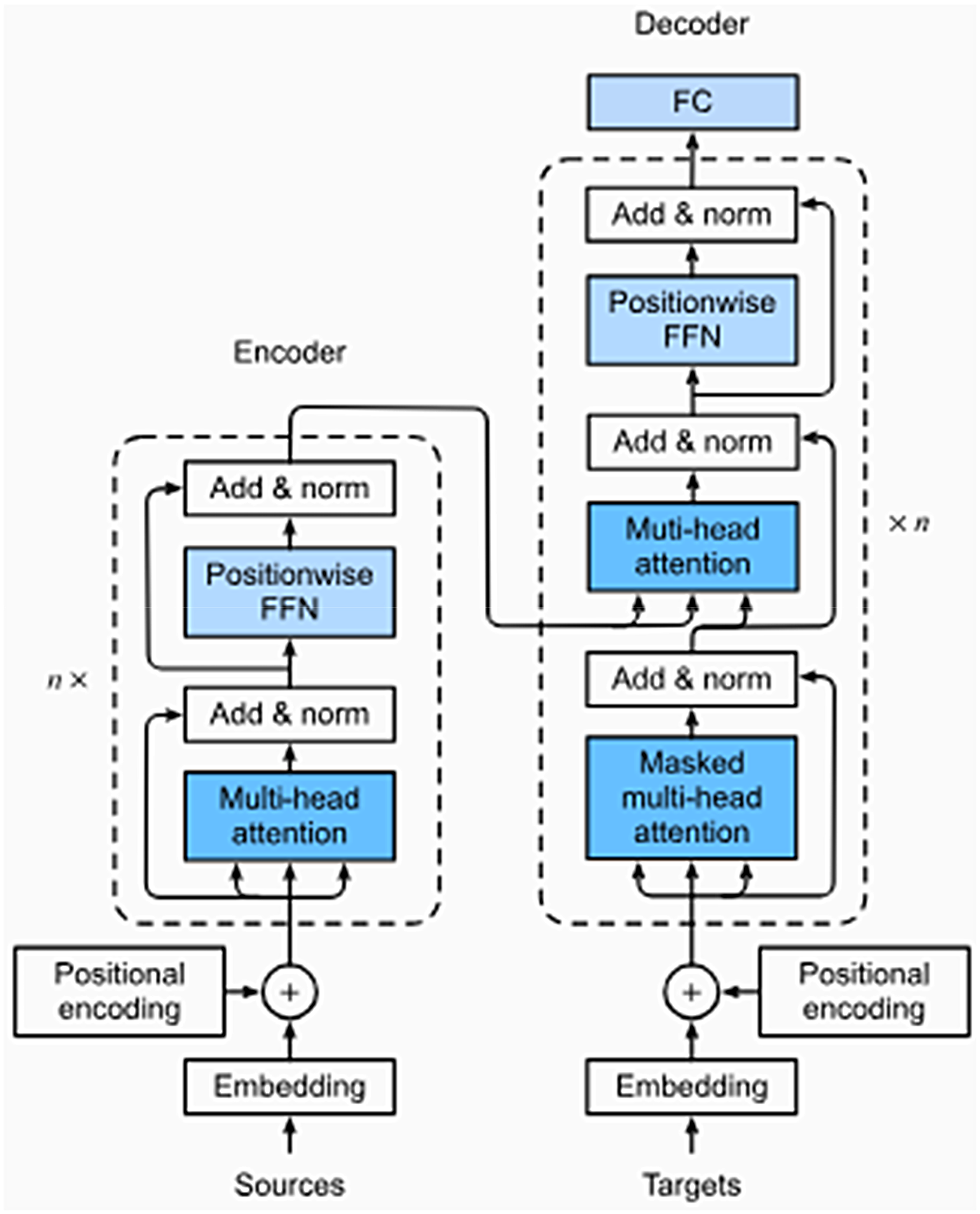
Transfer model architecture.

Encoder: The encoder in this architecture is composed of five distinct but interconnected layers, each playing an important part in processing the input set of data points throughout time. It starts with the input layer, which is where the raw data is converted into a high-dimensional vector by using a fully connected network in order to make use of a system for focusing the attention of several heads simultaneously. Applying encoded positions layer that uses functions that are sine and cosine helps to ensure that the data over time will continue to be organized throughout the correct sequential order. After that, a four-stage encoding procedure is performed on the resultant vector, which combines the information obtained from the input with the positional encoding. Following the completion of each encoding layer comes a series of normalization layers. These levels are comprised of a layer for self-attention as well as sublayer that is feed-forward and fully connected. This process culminates in the creation of a p-dimensional vector, which is subsequently passed to the decoder for further processing and interpretation of the time series data.

Decoder: In our decoder design, we closely adhere to the foundational architecture of the original Transformer model. A layer for input, four concurrent with layers for decoding and one for output are some of the essential components that make up the decoder module. The encoder's output is used for generate the input for the decoder, which then passes via the input layer to be transformed into a high-dimensional vector of length “n.” “n” refers to the number of bits in the vector. A third sublayer is added by the decoder, which comes in addition to the two necessary sublayers that are inherited from the encoder. This additional layer enhances the model's capacity to perform self-attention on the encoder's output. The decoder module is rounded out with an output layer, which serves the critical function of converting information from the top most decoder level in to the desired time sequence.

To ensure that predictions of future time series data points rely solely on prior data, we incorporate two vital mechanisms. The first mechanism, known as “look- ahead” masking, acts as a preventive measure, ensuring that the model doesn’t access future data when making predictions. These mechanisms involve maintaining the decoder's input and the target's output are off by one place. In practice, this means that the data points preceding the one being predicted are used as a reference, contributing of the model's ability to generate accurate forecasts based on historical context.

Firefly algorithm

The FFA metaheuristics, developed by Yang, draws inspiration from the bioluminescent and social behavior shown by fireflies. The FFA utilizes several approximations approaches to replicate the intricate and advanced characteristics of real-world natural systems. The luminosity and allure of fireflies are utilized to construct a fitness function, The attraction in most conventional implementations of the FFA is based on the luminescence, which is determined by the numerical value of the function called the objective (Bacanin et al., 2020). The formulation for minimizing the problem is as follows:

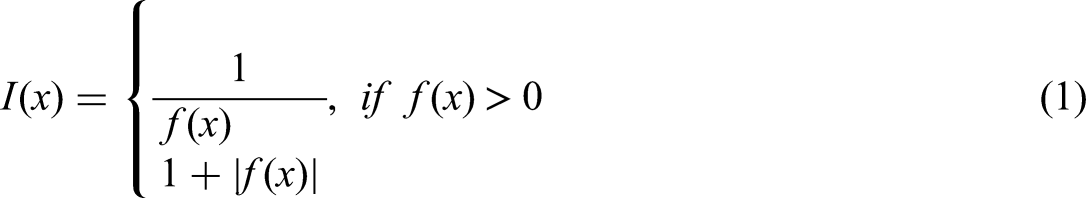
I (x) = {\frac{1}{\begin{matrix} f (x) \\ 1 + | f (x) | \end{matrix}}, i f f (x) > 0

(1)

I(x) is the measure of attractiveness, whereas f(x) reflects the value of the objective function at point x

The luminosity diminishes as the distance away from a light source augment, leading to a decline in the allure for people.

I (r) = \frac{I_{0}}{1 + γ r^{2}}

(2)

where I_0denotes the light brightness at the point of origin and I(r) denotes the light strength at distance r. Moreover, the FFA uses the γ parameter, which denotes the light absorption coefficient, to replicate actual natural systems in which light is partially absorbed by its surroundings. The next Gaussian form is used in most FFA versions to mimic the combined impact of the γ coefficient and the inverse square law of motion for distance.

I (r) = I_{0} . e^{- γ r^{2}}

(3)

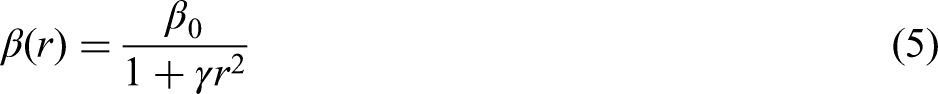
Furthermore, every firefly individual use attractiveness β, which is controlled by distance and closely associated with a firefly's light intensity, as shown in equation (4).

β (r) = β_{0} . e^{- γ r^{2}}

(4)

The parameter β0 represents the level of attraction when the distance r is equal to zero. It is important to mention that in practical applications, equation (4) is often substituted by equation (5).

β (r) = \frac{β_{0}}{1 + γ r^{2}}

(5)

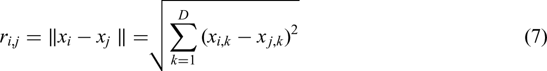
A search equation for an arbitrary individual i using the FFA, that shifts to a new location xi toward an individual j with superior fitness in each iteration t + 1, may be stated as follows:

x_{i}^{t + 1} = x_{i}^{t} + β_{0} . e^{- γ r_{i, j}^{2}} (x_{j}^{t} - x_{i}^{t}) + α^{t} (K - 0.5)

(6)

where the randomization parameter, represented by α, is the distance between two observed fireflies, U and j, and a random integer generated from a Gaussian or uniform distribution is represented by κ and r_r,i. For β0 and α, typical values that provide satisfactory outcomes for the majority of problems are 1 and [0, 1], respectively.

Cartesian distance, denoted by $r_{i, j}$ , is computed using equation (7).

r_{i, j} = ∥ x_{i} - x_{j} ∥ = \sqrt{\sum_{k = 1}^{D} {(x_{i, k} - x_{j, k})}^{2}}

(7)

where the number-specific issue parameters are indicated by D.

Generative adversarial networks

GAN, a potent class of generative models, achieves its purpose by implicitly modeling high-dimensional data distributions. Within the field of image processing, GANs possess the capability to generate high-quality images that closely resemble genuine ones, surpassing the performance of other generative techniques. Regarding its use in our research, GAN is utilized to get the statistical distribution of past solar irradiance data for ten distinct weather conditions. This enables us to generate additional instances of daily irradiance data based on the acquired distribution, which serves as one of the further responsibilities of GAN, specifically data augmentation (Wang et al., 2020a).

The GAN framework presented in Figure 2 is an integrated system that combines generative and adversarial networks. The training approach for a GAN involves learning two models: the generator G and the discriminator D (Capel, 2022). These are often constructed using neural networks that are deep, however they may also be created using any sort of distinguishable system that transforms data from one domain to another. In signal processing, vectors are typically denoted using bold, lowercase symbols, which is done to highlight the multidimensional aspect of variables. The distribution of the real data is represented by the probability density function p(x), where x is a random vector in the space R^g, with g being the number of dimensions.

Figure 2.

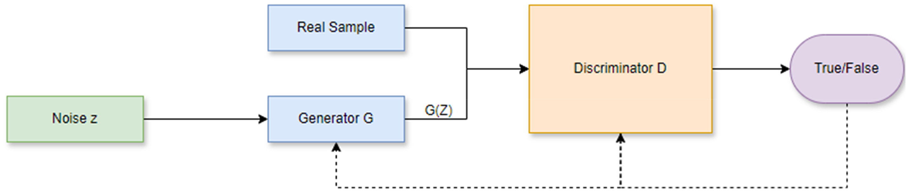
GAN framework.

There are some notable distinctions between the proposed framework and existing PV forecasting methodologies. Conventional models such as CNN, LSTM, ARIMA, or ensemble learning frameworks exhibit high sensitivity to noise and atmospheric variability due to their frequent reliance on raw or barely processed inputs. Our model's GAN-based denoising step dramatically improves input quality by reducing aberrations in sky pictures. Our approach use auto encoders and the FFA to retain only the most informative characteristics, hence enhancing model generalization, unlike prior studies that often extract extensive feature sets, which may include redundant or irrelevant data. Moreover, our AATL component selectively emphasizes significant spatiotemporal cues, enhancing accuracy relative to conventional models that do not have methods to prioritize dynamic and localized weather patterns. The superior predictive performance of our methodology can be attributed to these integrated improvements, which set it apart from prior methodologies.

Methodology

The proposed method effectively tackles the challenge of enhancing PV output prediction using a three-step procedure: image denoising, feature extraction, and AATL. Figure 3 shows the block diagram of the proposed method. The initial phase encompasses the resolution of disturbance present in sky images, a critical concern that can significantly impair the precision of prognostications. Here, GANs are of critical importance. In essence, GANs consist of a competition between two neural networks: the generator network endeavors to generate novel images that closely resemble authentic sky images, while the discriminator network differentiates between generated and real images. By acquiring the ability to eliminate noise from sky images through this iterative training process, the GANs enhance the quality of the data that is input into subsequent phases.

Figure 3.

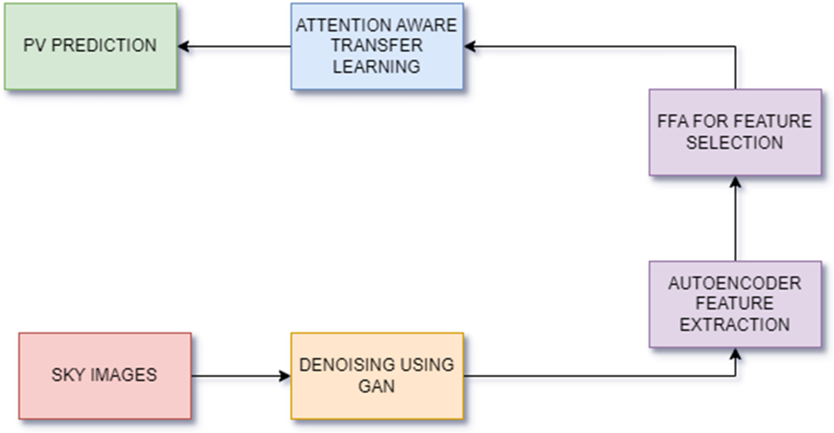
Block diagram of method.

From there, preprocessed images are fed into auto encoders; a neural network type that is trained to recognize a compressed representation of input data. An auto encoder is comparable to a skilled summarizer in its own right. It takes the image and condenses it so that only the most important parts are present in form of shorter versions. For instance, cloud cover patterns, atmospheric conditions, position of the sun in sky must be taken into consideration when making forecasts about PV output. Consequently, this approach uses auto encoders for taking such attributes from sky image data which can help predict accurately.

At last, the extracted features are incorporated into the AATL model. Thus, transfer learning is implemented. This approach utilizes a deep learning model that has been pretrained on a substantial volume of data as the foundation for the novel challenge of forecasting PV outputs. Furthermore, this pertained model has the capability to extract intricate features that are more informative and significant from the output of the auto encoder. Additionally, AATL's attention mechanism is utilized to enhance the prediction process. It illuminates those critical elements discovered during the feature extraction phase. The AATL model subsequently improves its PV output forecasts by concentrating on this pertinent data.

Dataset description

This dataset is unique among open-sourced datasets for deep learning studies on solar forecasting because it has two data tiers.

Benchmark dataset

This includes three years of sky images and PV power production data taken at 1-min intervals (6464), which can be used to build deep learning models.

Raw dataset

For different study objectives, sky video footage (2048 × 2048) and sky picture frames (2048 × 2048) have been combined with historical PV power production data collected at a rate of once per minute in order to generate overlapping datasets.

The data we collected at this website https://github.com/yuhao-nie/Stanford-solar-forecasting-dataset.

Preprocessing steps for image classification

To show the effect of well-known pre-processing techniques on accuracy of basic convolutional networks. The following are preprocessing steps:

Read image

Resize image

Smooth image

Find feature

Read image: After setting a variable to read the image, we were able to load arrays into our loaded folders which contained pictures.

Resize image: In order to see how resizing can affect an image, we will create two approaches showing one and two pictures. We then build a processor that takes photographs only.

Remove noise: To improve the input quality for upcoming predictive modeling by using GAN networks and sophisticated denoising algorithms to clear up noisy PV system data.

Feature extraction: During training, the auto encoder learns how to compress the input pictures into a feature vector. This captures the most significant aspects of the input photos, along with noise and superfluous or undesired features. Because of this, the compressed representation is often smaller than the original input, which makes it suitable for further processing. The auto encoder for Feature Extraction was specifically created to extract the most important features required to perform tasks such as denoising and picture defogging. Through crucial feature extraction, it advances to enhance later phases of the image processing pipeline and directs AATL or image denoising.

Feature selection: Utilizing the FFA, features were selected subsequent to their extraction. In the background segment, a comprehensive explanation of the algorithm is provided. A compact feature vector obtained from the input images using the FFA for feature selection, which attempts to extract essential characteristics. It not only improves subsequent phases in the image processing pipeline but also enables AATL and image denoising by giving precedence to the selection of relevant features during feature selection using the FFA.

Model building: AATL was incorporated into the model development procedure in this study. By leveraging on the utilization of a preexisting neural network framework (e.g. a CNN that had been trained in a comparable field, we refined the model in order to tailor its acquired representations to the particular challenge of forecasting PV output. By incorporating attention mechanisms into the model, we were able to give precedence to significant features and temporal dynamics, thereby augmenting its ability to discern complex patterns within the data.

Train test split

Our study dataset includes training and testing datasets to create machine learning models to enhance PV output prediction. Therefore, while training a model, utilize the biases and weights from the training set to capture the patterns and correlations essential for successful prediction. But the independent testing set helps objectively evaluate the model's ability to forecast PV production under changing circumstances.

Parameters from the training set help photovoltaic output prediction models generalize to new data. In this situation, training may improve model accuracy in forecasting PV outputs. However, train and test sets should be separated for constructing and testing models on fresh instances. Splitting data between training and testing sets is important to accurately evaluate machine learning models’ PV output predictions.

Performance metrics

The general objective of this research paper is to increase accuracy of PV output prediction using AATL and image denoising techniques. The study strives at improving the reliability of forecasting algorithms for PV output, which are vital in optimizing the solar energy utilization. Most importantly, the metrics considered in evaluating how the model predicts an outcome matters a lot because they influence the final outcome. Performance measures presented below can be used to compute error rate between predicted and actual values:

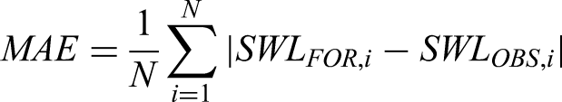
Mean absolute error

Moreover, these absolute discrepancies between predicted and actual output sums up to give us mean absolute error. Due to equal weights on all variables, it is not possible to establish whether it under or over forecasted. MAE formula is given as in equation below.

M A E = \frac{1}{N} \sum_{i = 1}^{N} | S W L_{F O R, i} - S W L_{O B S, i} |

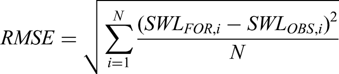
Root mean squared error

Finally, the equation shown next describes how average squared deviation between predicted and actual outputs helps decide which RMSE should be employed. In cases where there is a very nonlinear error this strategy is used. On other hand RMSE gives you an estimate of how wrong your predictions are; that is why it can be relied upon as a measure of accuracy in forecasting.

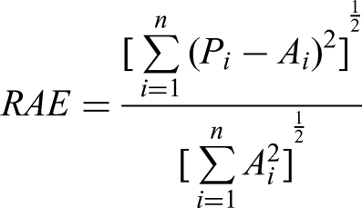
R M S E = \sqrt{\sum_{i = 1}^{N} \frac{{(S W L_{F O R, i} - S W L_{O B S, i})}^{2}}{N}}

Relative absolute error

The RAE calculates how much greater the error of a naive model's residuals or mean is than its forecast error. A value less than 1 is produced by equation if the new model outperforms the simple model. In equation (4), “P” represents expected value and “A” represents actual value.

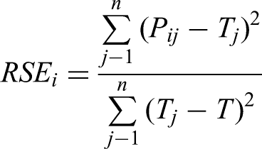
R A E = \frac{{[\sum_{i = 1}^{n} {(P_{i} - A_{i})}^{2}]}^{\frac{1}{2}}}{{[\sum_{i = 1}^{n} A_{i}^{2}]}^{\frac{1}{2}}}

Root-relative squared error

Finally, the equation shown next describes how average squared deviation between predicted and actual outputs helps decide which RMSE should be employed. In cases where there is a very non-linear error this strategy is used. On other hand RMSE gives you an estimate of how wrong your predictions are; that is why it can be relied upon as a measure of accuracy in forecasting.

R S E_{i} = \frac{\sum_{j - 1}^{n} {(P_{i j} - T_{j})}^{2}}{\sum_{j - 1}^{n} {(T_{j} - T)}^{2}}

\bar{T} = \frac{1}{n} \sum_{j = 1}^{n} T_{j}

Tools and software's for analysis

We used the programming language Python for our investigation, taking use of its vast ecosystem of analysis of data, machine learning, and deep learning modules. In addition, Google Colab served as our main computing platform.

Results

Generative adversarial network

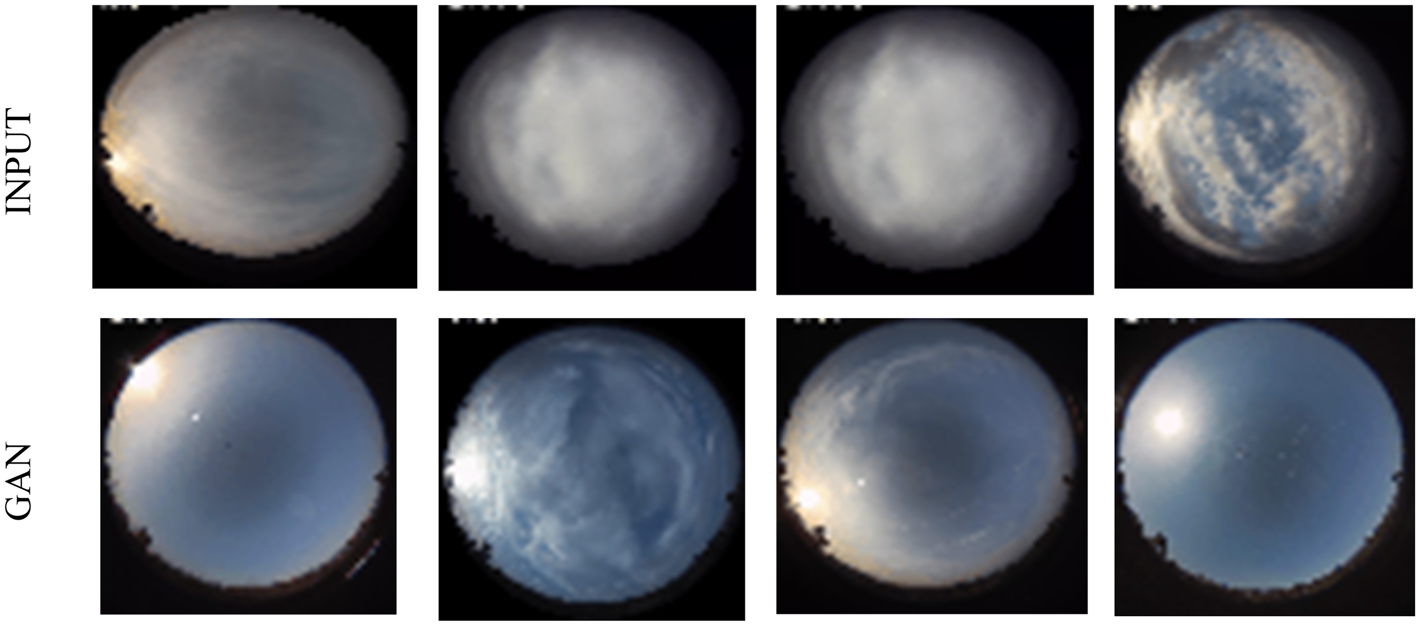
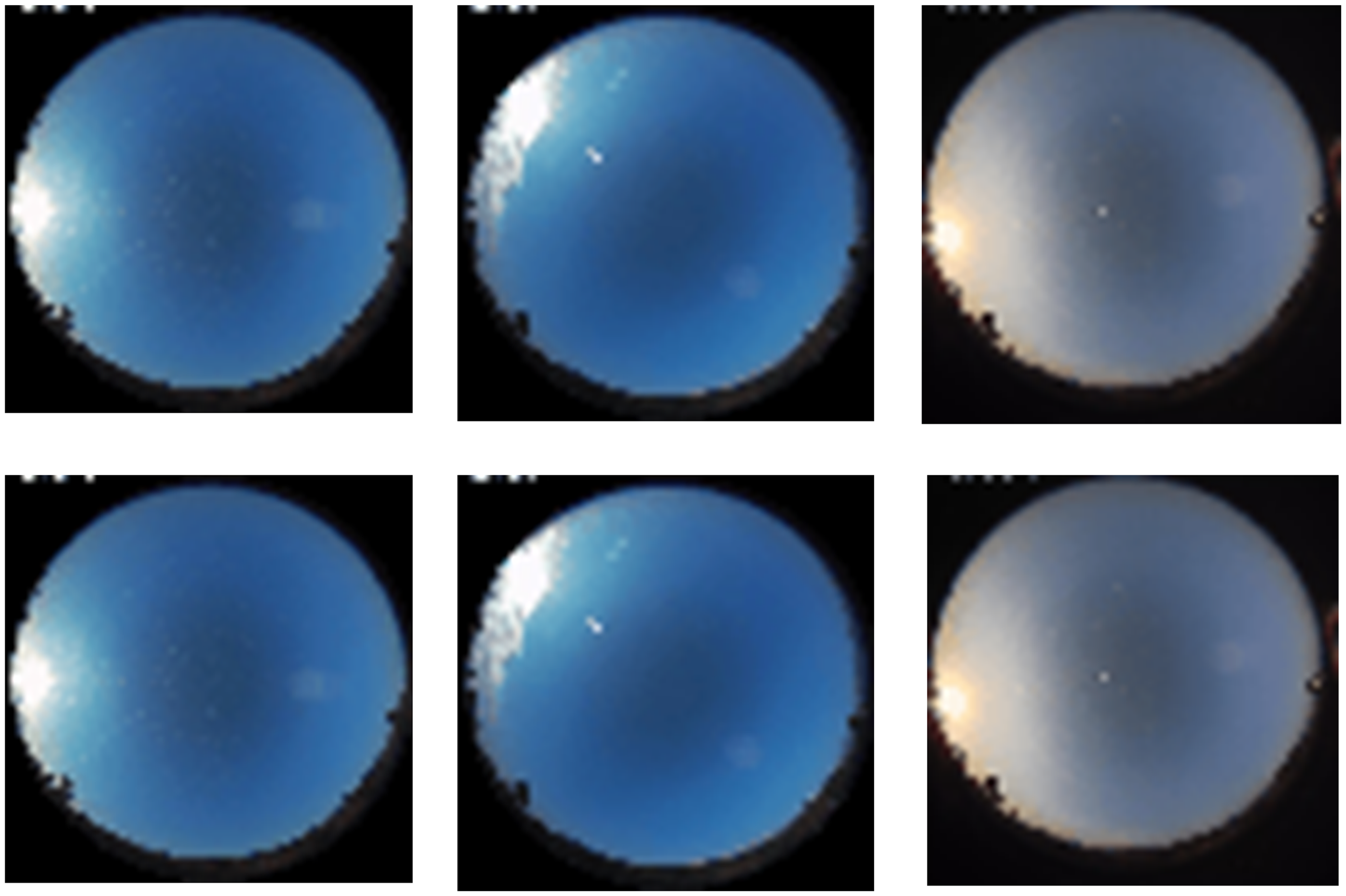
Figure 4 illustrates the efficacy of the GAN in preparing sky pictures for PV forecasting. The unprocessed sky photos, sourced straight from the dataset and shown in the top row (“INPUT”), sometimes exhibit noise, cloud distortion, and light unpredictability, which may compromise forecast accuracy. Subsequent to denoising by GAN, the relevant pictures are shown in the lower row (“GAN”). The GAN-based processing effectively removes extraneous noise, enhances structural clarity, and facilitates the visibility of significant atmospheric elements such as cloud borders and sunshine intensity. GAN mitigates error propagation within the forecasting framework by producing cleaner and more representative input pictures, significantly enhancing the reliability of subsequent feature extraction and prediction phases.

Figure 4.

GAN output.

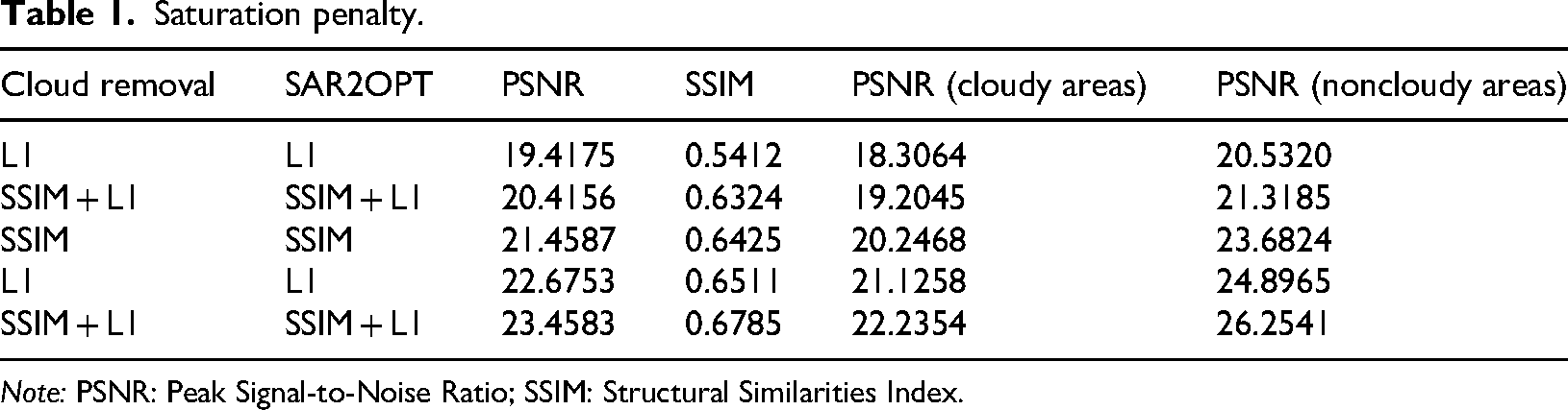
Table 1 illustrates the effectiveness of several cloud removal approaches evaluated by Peak Signal-to-Noise Ratio (PSNR) and Structural Similarities Index (SSIM). The SSIM + L1 combination yields optimal performance (PSNR = 23.4583, SSIM = 0.6785), with GAN-based approaches regularly surpassing unprocessed hazy pictures. Significantly, GAN pretreatment enhances structural integrity and reduces noise, yielding more reliable picture quality, as shown by PSNR values for both cloudy and noncloudy areas. These advancements illustrate the significance of GAN-based denoising in producing cleaner input data, which immediately improves the accuracy of PV output prediction.

Table 1.

Saturation penalty.

Cloud removal	SAR2OPT	PSNR	SSIM	PSNR (cloudy areas)	PSNR (noncloudy areas)
L1	L1	19.4175	0.5412	18.3064	20.5320
SSIM + L1	SSIM + L1	20.4156	0.6324	19.2045	21.3185
SSIM	SSIM	21.4587	0.6425	20.2468	23.6824
L1	L1	22.6753	0.6511	21.1258	24.8965
SSIM + L1	SSIM + L1	23.4583	0.6785	22.2354	26.2541

Note: PSNR: Peak Signal-to-Noise Ratio; SSIM: Structural Similarities Index.

PSNR (cloudy areas): This column most likely shows the PSNR measure that was especially determined for the cloud-covered portions of the picture. In this case, a greater PSNR value indicates better picture quality retention in the foggy areas after cloud removal.

PSNR (noncloudy regions): The PSNR metric computed for the image's unaffected regions is shown in this column. After the removal procedure, a greater PSNR value here indicates better picture quality retention in the cloud-free areas.

L1 and SSIM: These columns show how the L1 loss and SSIM measurements are used separately, respectively. While SSIM assesses how comparable the structures in the pictures are, L1 loss quantifies the absolute pixel-by-pixel changes between the original and reconstructed images.

SSIM + L1: This column shows a combination method for cloud removal that makes use of both L1 loss and SSIM. By combining these measures, the original and reconstructed pictures’ pixel-by-pixel and structural similarities are probably intended to be taken advantage of.

SSIM: Without considering L1 loss, this column presumably represents the outcomes derived exclusively through the utilization of the SSIM metric for cloud removal.

L1 SSIM + L1 and SSIM + L1: These columns show integrated methods for cloud removal that use both SSIM and L1 loss. The specifics of how these two are implemented or the weights given to each measure throughout the optimization process may be the difference between them.

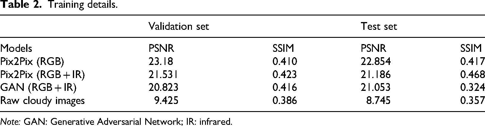
Table 2 contrasts several GAN-based training methodologies. Compared to unprocessed cloudy photos (PSNR = 9.425, SSIM = 0.386), models trained using Pix2Pix (RGB) get superior PSNR (23.18 validation, 22.854 test) and SSIM (0.410 validation, 0.417 test). The findings indicate a significant improvement compared to raw photos, however including infrared (IR) data into Pix2Pix (RGB + IR) and GAN (RGB + IR) somewhat reduces PSNR and SSIM. These findings confirm that GAN pretreatment enhances the structural integrity and clarity of pictures, allowing more accurate downstream feature extraction and bolstering the robustness of solar forecasting models.

Table 2.

Training details.

	Validation set		Test set
Models	PSNR	SSIM	PSNR	SSIM
Pix2Pix (RGB)	23.18	0.410	22.854	0.417
Pix2Pix (RGB + IR)	21.531	0.423	21.186	0.468
GAN (RGB + IR)	20.823	0.416	21.053	0.324
Raw cloudy images	9.425	0.386	8.745	0.357

Note: GAN: Generative Adversarial Network; IR: infrared.

When opposed to using raw, foggy photos, the use of adaptive adversarial networks (GANs)—such as Pix2Pix and GAN—in image processing produces noticeably better results for the SSIM and PSNR. This shows that adding in IR data may introduce excess noise, or cause other problems for this model.

The inclusion of the IR data in Pix2Pix (RGB + IR) has led to slightly lower PSNR and SSIM compared to Pix2Pix (RGB) in Table 2. This indicates that including IR might bring about more noise or difficulties for this particular model.

Among the models using GANs, this model has the lowest PSNR but has SSIM similar to Pix2Pix (RGB). This means that GAN can be very good at retaining structural complexities, though it will add more noises than any other models.

Generally, the table highlights how GANs can help reduce noises in images for solar production prediction. Additionally, it illustrates why the best performance is reached when we select a right model and data combination (RGB vs RGB + IR).

For evaluation of our model's efficacy, we used various performance metrics as given in figures presented below. Some of these metrics are mentioned: MAE, RAE and MSE are three common metrics used to measure accuracy of a model. It is possible to conduct a thorough evaluation of the accuracy and effectiveness of the model in predicting solar power energy by using these metrics, based on the chosen characteristics and methodology. Feature extraction results were shown in Figure 5 using encoder and decoder.

Figure 5.

Corresponding outputs of encoder and decoder.

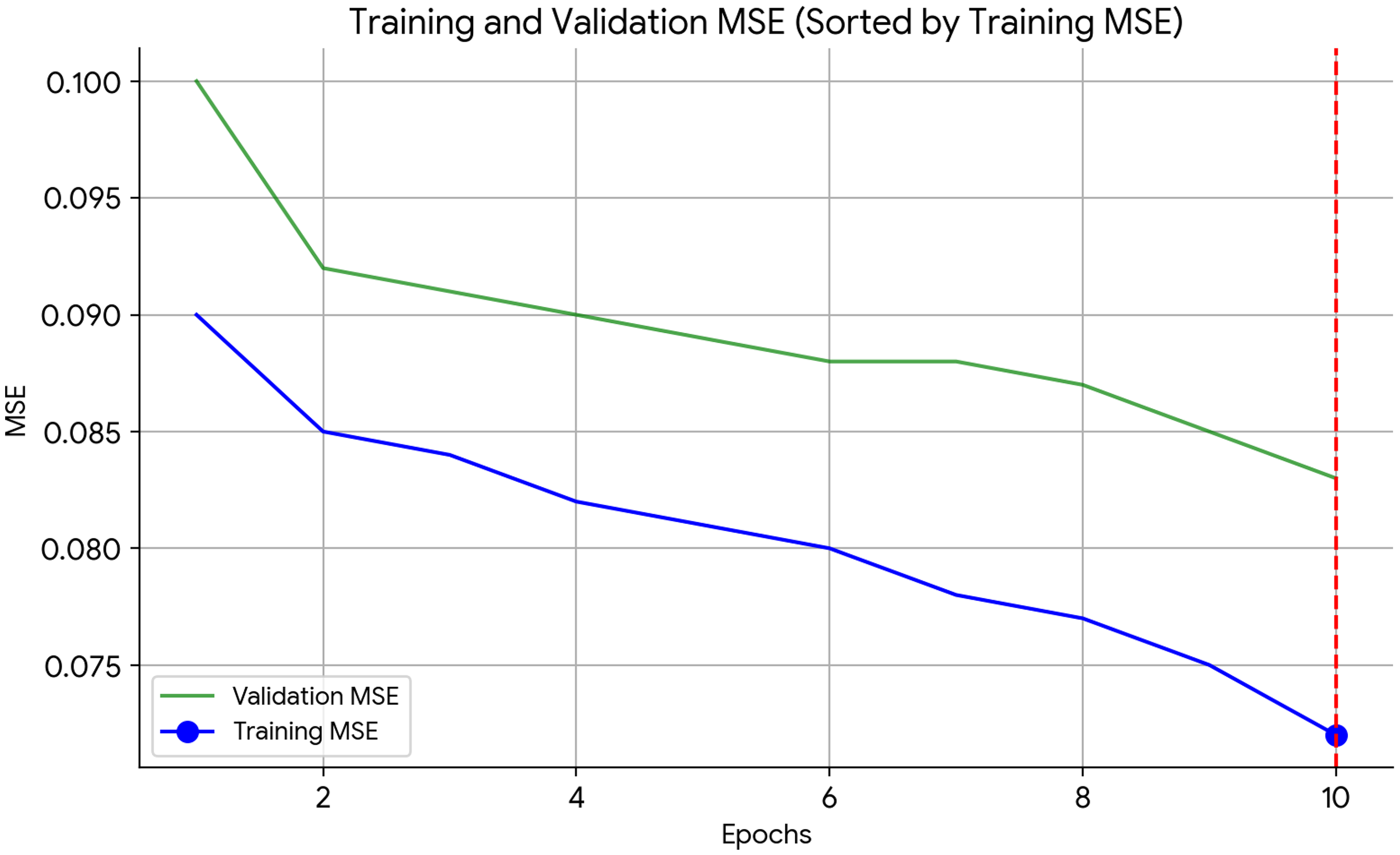
The MSE for the training and validation sets throughout the epochs of a machine learning training procedure is illustrated in this graph shown in Figure 6. The MSE is exhibited along the y-axis in order to show how well the model fits the data, while the total number epochs is indicated along the x-axis. A lower MSE indicates a better match. Our absolute objective is to reduce the MSE.

Figure 6.

MSE over number of epochs in training.

The diagram in Figure 6 exhibits two curves. Training MSE (circled blue line). This line indicates the MSE for the data used in training. As the model gains knowledge of patterns from the training data, it generally diminishes. The circle marker denotes the epoch in which the minimum value of the training MSE is observed.

The validation MSE (green line) signifies the MSE obtained from an independent validation set, which the model did not access during training. It helps in determining how effectively the model adapts to fresh data. While it should ideally drop during training, if the model overfits the training data, the validation MSE may start to rise. The training MSE in this particular plot displays a general downward trend with some fluctuations, with its minimal value occurring around epoch 170. Although the validation MSE exhibits a decline, it maintains an invariant value higher than the training MSE. This indicates the possibility of overfitting, in which the model becomes overly dependent on the training data, possibly to the detriment of its ability to generalize.

Although the absolute MSE values are not ascertainable as a result of the nonzero y-axis scale, the plot nonetheless offers significant insights. Extending the view of the validation MSE over a longer period of time would be advantageous for the limited x-axis that only displays 10 epochs (training generally encompasses hundreds or thousands). The figure indicates that the model is effectively assimilating the training data, however overfitting may be an issue.

The training hyper parameters are described in Table 3.

Table 3.

Training hyperparameters.

Software framework	Keras
Optimizer	Adam
Learning data	0.001
Number of epochs	10
Batch size	64
Activation function	“Relu” for all hidden layers “Sigmoid” for the output layer
Convolutional kernel size	3 × 3
Max-pooling kernel size	2 × 2
Up-sampling kernel size	2 × 2
Training samples (70%)	17,680
Validation samples (15%)	3789
Testing samples (15%)	3789

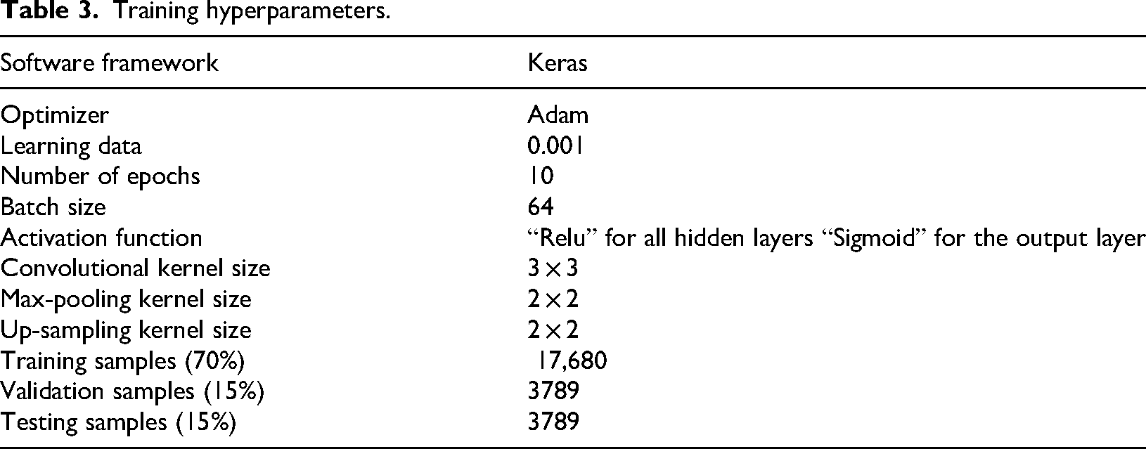
The hyperparameter settings used to optimize the training of the proposed model are shown in Table 3. The Adam optimizer, with a batch size of 64 and a learning rate of 0.001, ensured stable convergence throughout training. The Sigmoid output activation was appropriate for the prediction task, whereas the Relu activation function in buried layers facilitated effective nonlinear feature extraction. A balanced framework for model learning and assessment was established by selecting 10 epochs with a distribution of 70% for training, 15% for validation, and 15% for testing. The proposed method's dependability was shown by the constant reduction in error metrics across the datasets facilitated by these parameter selections.

Relative absolute error

The bar graph in Figure 7 displays the RAE across several forecasting models. The x-axis of the graph displays the several models that were used. This collection contains the following models: CNN, LSTM, ARIMA, and AATL. The graph's RAE is shown on the vertical axis. A forecast's deviation from the actual value is measured by the RAE. The smaller the RAE, the more accurate the prediction. According to the chart, the smallest RAE of 0.110131087 is seen in AATL model which is followed by Autoregressive integrated moving average and CNN models. The LSTM model has high relative absolute inaccuracy. The graph indicates that Focus Aware learning transfer model performs better as compared to other model in terms of accuracy of prediction.

Figure 7.

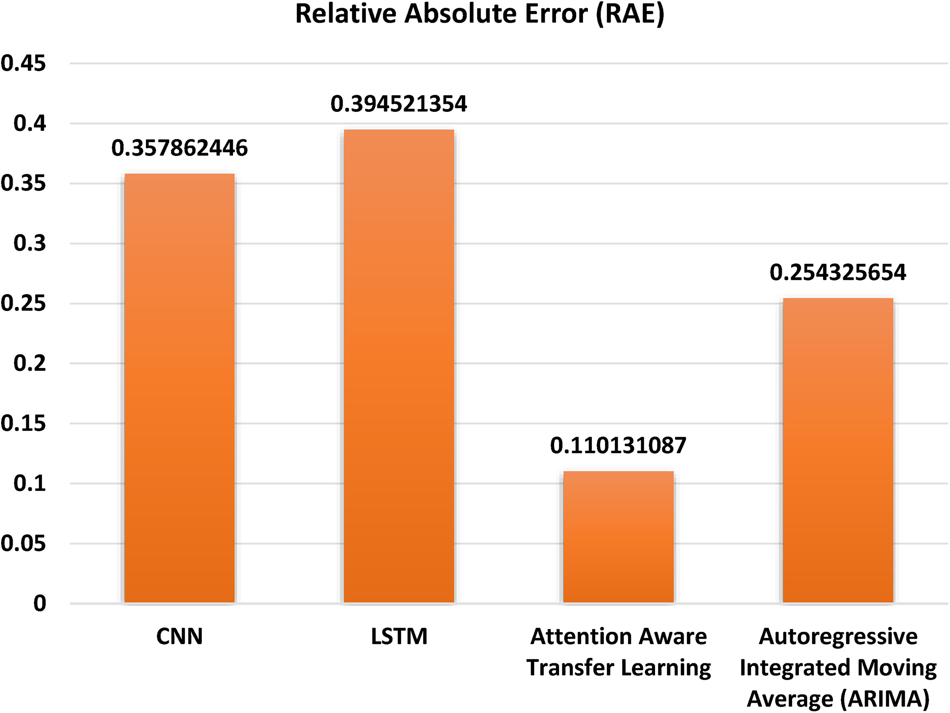
Relative absolute error.

Root mean squared error

The graph in Figure 8 shows various root averaged squared errors for different approaches such as ARIMA, CNN, LSTM, and AATL. The vertical axis on the graph denotes RMSE. In addition, it has a recommended Attention aware transfer model that displays remarkable accuracy with very low RMSE rate of 0.1435456785. Therefore, it can be inferred that attention aware transfer model is the best appropriate model for predicting PV output.

Figure 8.

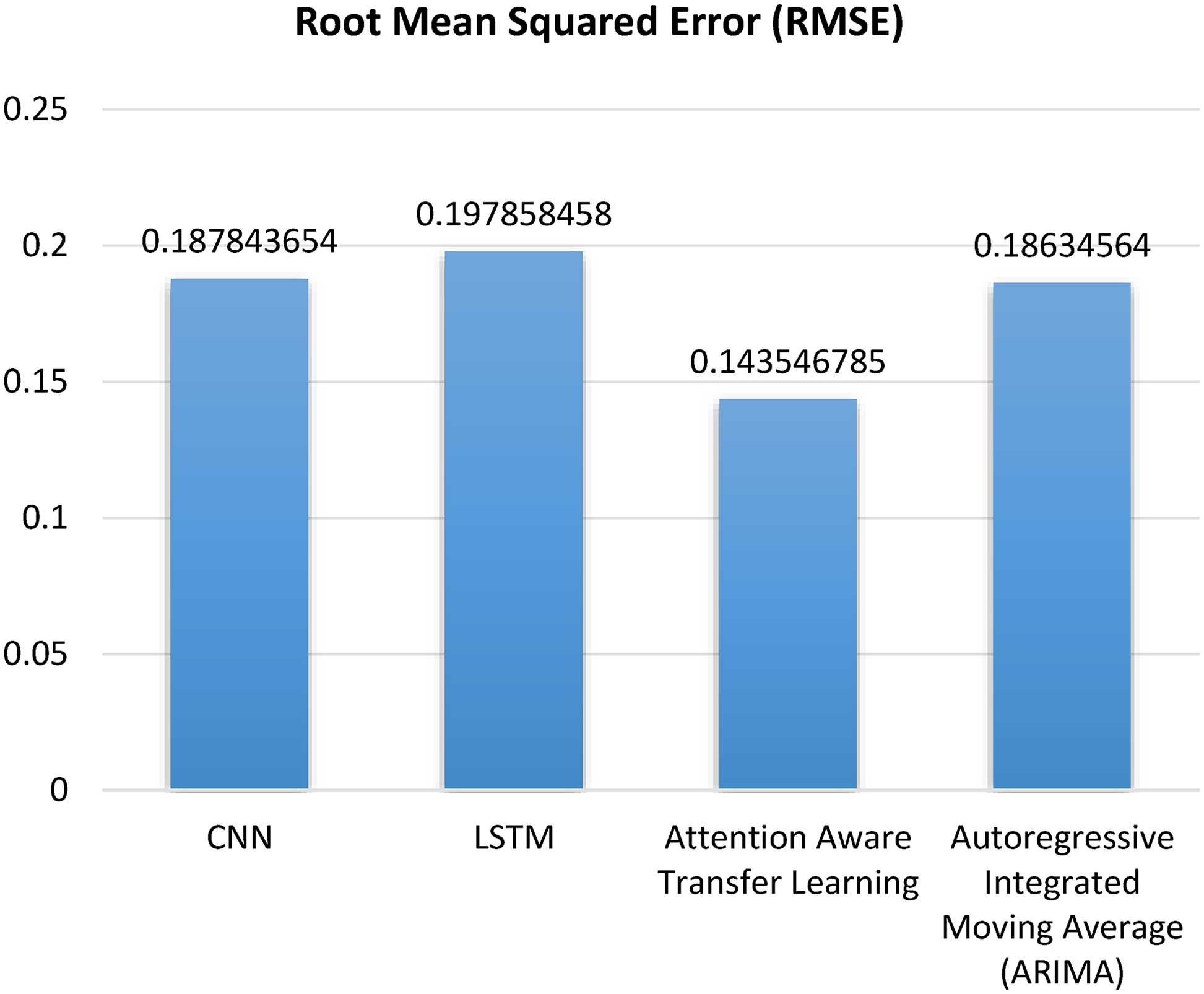
Root mean squared error.

Mean absolute error

A bar graph in Figure 9 displaying the MAE for some machine learning methods is given. By summing up the absolute discrepancies between the expected and actual values, we can get the MAE. Simply put, it is a measure of how far wrong predictions made by a machine learning model are. Models with low MAE numbers have a higher level of accuracy. On the x-axis of this graph are machine learning techniques that were compared. The ARIMA, CNN, LSTM and AATL are some of them. The vertical axis on this plot represents MAE. Based on the graph, the LSTM model has the highest MAE, indicating that it has the greatest disparity between its predictions and the actual values. The AATL model achieves the lowest MAE, indicating that it exhibits the least discrepancy between its predicted values and the actual values.

Figure 9.

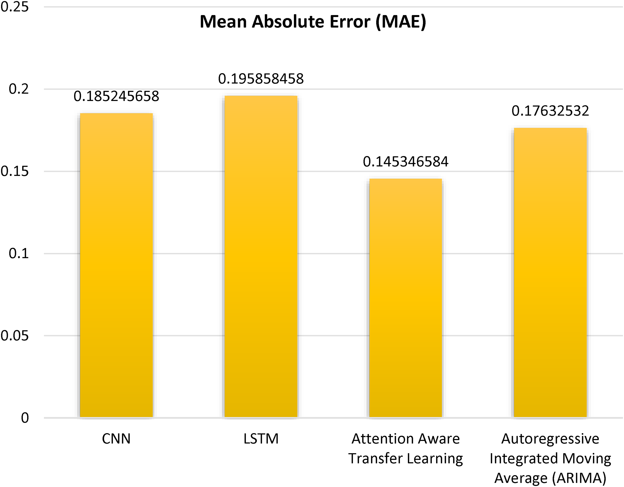
Mean absolute error.

Root relative squared error

In Figure 10 bar graph that displays the average Root Comparative Taking Error for several models. The forecasting accuracy is gauged using the RRSE metric. A more accurate prediction is indicated by a lower RRSE. The bar graph shows that the suggested Attention aware transfer model demonstrates superior accuracy, with a very low root relative squared error rate of 0.135426575. Therefore, it can be inferred that the attention aware transfer model is the optimal model for predicting PV output.

Figure 10.

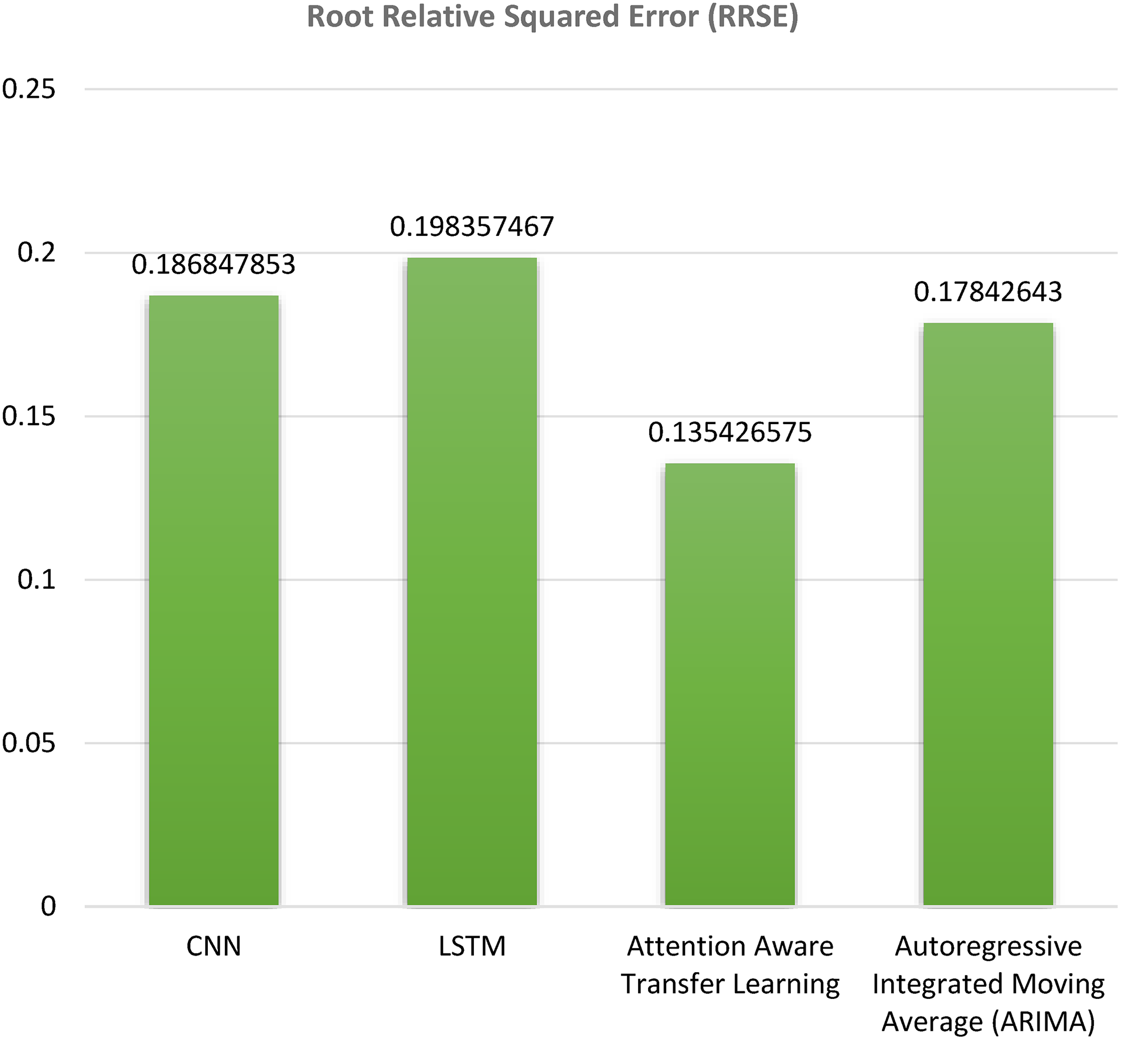
Root relative squared error.

Discussion

The proposed AATL paradigm outperforms conventional models such as CNN and LSTM for many significant reasons. Initially, by removing ambient noise from the input data, the GAN-based picture denoising process improves quality and hence reduces error propagation during prediction. Secondly, auto encoder-based feature extraction eliminates redundant features that often lead to overfitting in CNN or LSTM models, yielding compact and highly informative representations that encapsulate atmospheric conditions and cloud patterns. The FFA enhances the model's capacity to generalize across various weather situations by retaining just the most relevant information. Finally, AATL's attention method dynamically emphasizes significant spatiotemporal dependencies, such as sudden cloud movements, which standard CNN and LSTM models struggle to effectively capture because to their static feature learning capabilities. This advantage is also corroborated by a detailed analysis of the error measures. The continuously reduced MAE, RMSE, RAE, and RRSE values achieved by AATL indicate its capability to limit variability across diverse meteorological circumstances and temporal horizons while also decreasing average error. CNN and LSTM models have increased error variance, reflecting their vulnerability to noisy inputs and difficulties in capturing long-range temporal connections. The proposed AATL framework is deemed more dependable and adaptable based on this error analysis, making it more suitable for actual PV forecasting applications.

Conclusion

This study introduces an innovative and cohesive framework for forecasting PV output, integrating AATL for adaptive spatiotemporal modeling, auto encoders for efficient feature extraction, the FFA for optimal feature selection, and GANs for image denoising. The proposed approach significantly enhances the resilience and precision of PV forecasting by addressing persistent challenges such as noisy sky photos, redundant feature sets, and inadequate flexibility to changing environmental circumstances. The framework regularly surpasses conventional models, including CNN, LSTM, and ARIMA, based on experimental assessments across many error metrics (MAE, RMSE, RAE, RRSE). The improved performance is attributed to the synergistic interaction of intelligent feature prioritization, dynamic attention mechanisms, compact feature extraction, and GAN-based preprocessing, which together allow the model to more effectively capture significant atmospheric and temporal variations than traditional methods. The use of a publicly available benchmark dataset in this study ensures transparency, repeatability, and application for future research, constituting additional strength. In addition to its academic value, the framework aids grid management and solar energy operators by enhancing the reliable incorporation of PV electricity into energy markets and supporting the broader transition to sustainable energy systems.

Footnotes

ORCID iDs

Mohit Bajaj

Olena Rubanenko

Author contributions

Rahul Saraswat: conceptualization, methodology, software, visualization, investigation, writing—original draft preparation; Mohit Bajaj: data curation, validation, supervision, resources, writing—review and editing; and Olena Rubanenko: project administration, supervision, resources, and writing—review and editing.

Funding

The authors received no financial support for the research, authorship, and/or publication of this article.

Declaration of conflicting interests

The authors declared no potential conflicts of interest with respect to the research, authorship, and/or publication of this article.

Availability of data and materials

The datasets used and/or analyzed during the current study available from the corresponding author on reasonable request.

References

Abbas

Che

Maqsood

, et al. (2025) Self-adaptive evolutionary neural networks for high-precision short-term electric load forecasting. Scientific Reports 15(1): 21674.

Al-Dahidi

(2019) Ensemble_Approach_of_Optimized_Artificial LR(2).pdf.crdownload.

Al-Dahidi

Ayadi

Alrbai

, et al. (2019) Ensemble approach of optimized artificial neural networks for solar photovoltaic power prediction. IEEE Access 7: 81741–81758.

AlKandari

Ahmad

(2024) Solar power generation forecasting using ensemble approach based on deep learning and statistical methods. Applied Computing and Informatics 20(3/4): 231–250.

Atiea

Shaheen

Alassaf

, et al. (2024) Enhanced solar power prediction models with integrating meteorological data toward sustainable energy forecasting. International Journal of Energy Research 2024(1): 8022398.

Bacanin

Venkatachalam

Bezdan

, et al. (2020) Since January 2020 Elsevier has created a COVID-19 resource centre with free information in English and Mandarin on the novel coronavirus COVID-19. The COVID-19 resource centre is hosted on Elsevier Connect, the company’s public news and information website. Elsevier hereby grants permission to make all its COVID-19-related research that is available on the COVID-19 resource centre - including this research content - immediately available in PubMed Central and other publicly funded repositories, such as the WHO COVID database with rights for unrestricted research re-use and analyses in any form or by any means with acknowledgement of the original source . These permissions are granted for free by Elsevier for as long as the COVID-19 resource centre remains active. Microprocessors and Microsystems A novel firefly algorithm approach for efficient feature selection with COVID-19 dataset.

Bashir

Wang

Tahir

, et al. (2025) Wind and solar power forecasting based on hybrid CNN-ABiLSTM, CNN-transformer-MLP models. Renewable Energy 239: 122055.

Blinov

Zaitsev

Bajaj

, et al. (2025) Advanced long short-term memory-based forecasting of electricity imbalances in the Ukrainian power system: Enhancing accuracy and stability with comparative model analysis. Energy Exploration & Exploitation: 01445987251360272.

Bui Duy

Nguyen Quang

Doan Van

, et al. (2024) Refining long short-term memory neural network input parameters for enhanced solar power forecasting. Energies 17(16): 4174.

10.

Capel

(2022) Denoising diffusion probabilistic models applied to energy forecasting in power systems .

11.

Djeldjeli

Taouaf

Alqahtani

, et al. (2024) Enhancing solar power forecasting with machine learning using principal component analysis and diverse statistical indicators. Case Studies in Thermal Engineering 61: 104924.

12.

Fabel

Nouri

Wilbert

, et al. (2022) Applying self-supervised learning for semantic cloud segmentation of all-sky images. Atmospheric Measurement Techniques 15(3): 797–809.

13.

Guermoui

Fezzani

Mohamed

, et al. (2024) An analysis of case studies for advancing photovoltaic power forecasting through multi-scale fusion techniques. Scientific Reports 14(1): 6653.

14.

Huang

Kuo

(2019) Multiple-input deep convolutional neural network model for short-term photovoltaic power forecasting. IEEE Access 7: 74822–74834.

15.

Khan

Walker

Zeiler

(2022) Improved solar photovoltaic energy generation forecast using deep learning-based ensemble stacking approach. Energy 240: 122812.

16.

Kheldoun

Merabet

Belmadani

, et al. (2024, February) Seasonal forecasting of global horizontal irradiance for grid-connected PV plants: A combined CNN-BiGRU approach. In: 2024 3rd International Conference on Power Electronics and IoT Applications in Renewable Energy and its Control (PARC), pp.169–173: IEEE.

17.

Khelifi

Guermoui

Rabehi

, et al. (2023) Short-term PV power forecasting using a hybrid TVF-EMD-ELM strategy. International Transactions on Electrical Energy Systems 2023(1): 6413716.

18.

Lee

Kim

(2019) Recurrent neural network-based hourly prediction of photovoltaic power output using meteorological information. Energies 12(2): 215.

19.

Wen

Tseng

, et al. (2019) Renewable energy prediction: A novel short-term prediction model of photovoltaic output power. Journal of Cleaner Production 228: 359–375.

20.

Zhang

, et al. (2021) A multi-step ahead photovoltaic power prediction model based on similar day, enhanced colliding bodies optimization, variational mode decomposition, and deep extreme learning machine. Energy 224: 120094.

21.

Lin

Tseng

, et al. (2020) An improved moth- flame optimization algorithm for support vector machine prediction of photovoltaic power generation. Journal of Cleaner Production 253: 119966.

22.

Wang

Zhou

, et al. (2024, August) Fusionsf: Fuse heterogeneous modalities in a vector quantized framework for robust solar power forecasting. In: Proceedings of the 30th ACM SIGKDD Conference on Knowledge Discovery and Data Mining, pp.5532–5543.

23.

Mfetoum

Ngoh

Molu

RJJ

, et al. (2024) A multilayer perceptron neural network approach for optimizing solar irradiance forecasting in Central Africa with meteorological insights. Scientific Reports 14(1): 3572.

24.

Molu

RJJ

Tripathi

Mbasso

, et al. (2024) Advancing short-term solar irradiance forecasting accuracy through a hybrid deep learning approach with Bayesian optimization. Results in Engineering 23: 102461.

25.

Mouloud

Kheldoun

Merabet

, et al. (2024) Assessment of hybrid bidirectional deep learning models for short-term global horizontal irradiance forecasting. AIP Conference Proceedings 3214(1): 020034. AIP Publishing LLC.

26.

Perera

De Hoog

Bandara

, et al. (2024) Day-ahead regional solar power forecasting with hierarchical temporal convolutional neural networks using historical power generation and weather data. Applied Energy 361: 122971.

27.

Singh

Kumar

Bajaj

, et al. (2024) Machine learning-based energy management and power forecasting in grid-connected microgrids with multiple distributed energy sources. Scientific Reports 14(1): 19207.

28.

Singh

Gupta

, et al. (2025) Forecasting rooftop photovoltaic solar power using machine learning techniques. Energy Reports 13: 3616–3630.

29.

, et al. (2023) FEPVNet: A network with adaptive strategies for cross-scale mapping of photovoltaic panels from multi-source images. Remote Sensing 15(9): 1–21.

30.

Venkateswaran

Cho

(2024) Efficient solar power generation forecasting for greenhouses: A hybrid deep learning approach. Alexandria Engineering Journal 91: 222–236.

31.

Wang

Xuan

Zhen

, et al. (2020a) A minutely solar irradiance forecasting method based on real-time sky image-irradiance mapping model. Energy Conversion and Management 220: 113075.

32.

Wang

Zhang

Liu

, et al. (2020b) Neural networks based weather classification.

33.

Zafar

Ahsan

Yousaf

, et al. (2025) Enhanced solar power forecasting in smart grids using a hybrid autoencoder and long short-term memory model. Energy Exploration & Exploitation: 01445987251360490.

34.

Zhang

(2021) Deep network based on up and down blocks using wavelet transform and successive multi-scale spatial attention for cloud detection. Remote Sensing of Environment 261: 112483.

35.

Zhang

Yan

Liu

(2024) Power generation forecasting for solar plants based on dynamic Bayesian networks by fusing multi-source information. Renewable and Sustainable Energy Reviews 202: 114691.

36.

Zhou

Gong

, et al. (2020) Prediction of photovoltaic power output based on similar day analysis, genetic algorithm and extreme learning machine. Energy 204: 117894.

37.

Ziane

, et al. (2021) Photovoltaic output power performance assessment and forecasting : impact of meteorological variables. Solar Energy 220(March): 745–757.

Enhanced photovoltaic output prediction through attention-aware transfer learning and image denoising

Abstract

Keywords

Introduction

Related work

Background

Transformer model

Model architecture

Firefly algorithm

Generative adversarial networks

Methodology

Dataset description

Benchmark dataset

Raw dataset

Preprocessing steps for image classification

Train test split

Performance metrics

Mean absolute error

Root mean squared error

Relative absolute error

Root-relative squared error

Tools and software's for analysis

Results

Generative adversarial network

Relative absolute error

Root mean squared error

Mean absolute error

Root relative squared error

Discussion

Conclusion

Footnotes

ORCID iDs

Author contributions

Funding

Declaration of conflicting interests

Availability of data and materials

References