Sage Journals: Discover world-class research

Abstract

Intelligent fault diagnosis using deep learning has achieved much success in recent years. Using deep learning method to diagnose bearing fault requires designing an appropriate neural network model and then train with a massive data. On the one hand, up to now, a variety of neural network structures have been proposed for different diagnostic tasks, but there is a lack of research of unified structure. On the other hand, the fault data of the training neural network are collected from the fault location point, which is quite different from the actual data, because the sensor cannot be located at the fault location point accurately. This paper attempts to design a unified neural network structure based on Resnet and improve the generalization performance by using transfer learning techniques. The effectiveness of the proposed method in this paper is verified using experiment under different working loads and non-fault location point.

Keywords

Intelligent fault diagnosis deep learning non-fault location point bearing fault

Introduction

Bearing is an important component of mechanical equipment, and its health will have a great impact on the overall safety performance of machinery.^1,2 Therefore, bearing fault diagnosis is an important research content.

In the past few years, bearing fault diagnosis methods have developed rapidly. Many researches have proposed various intelligent diagnosis algorithms combining feature extraction methods and pattern classification. Zhang and Zhou³ and Peng et al.⁴ improved ensemble empirical mode decomposition (EEMD) and Hilbert-Huang transform (HHT) methods, respectively, for bearing fault diagnosis. Yan et al.⁵ and Lei et al.⁶ reviewed the application of wavelet analysis and empirical mode decomposition (EMD) in fault diagnosis, respectively. Her-Terng et al.^7–9 studied ball-bearing fault diagnosis based on chaotic system and fractal theory. Although these algorithms improve the classification accuracy and efficiency of bearing fault diagnosis greatly, in the era of large data, to face complex mechanical systems and massive monitoring data, traditional intelligent diagnosis algorithms may have lost their advantages because of the limitations of applicability. In the era of big data, the deep learning methods developed in recent years have been widely used in many important fields.^10,11 In bearing fault diagnosis, exploring the use of deep learning algorithm to solve different problems has become a hot research issue.

Gan et al.¹² used the deep belief network (DBN) to classify the bearing faults, and they found that the diagnostic accuracy was significantly improved compared with the traditional back propagation neural network (BPNN) and support vector machine (SVM) methods. Wei et al.¹³ studied and designed the convolutional neural network named Deep Convolutional Neural Networks with Wide First-layer Kernels (WDCNN) and Convolution Neural Networks with Training Interference (TICNN)¹⁴ to solve the problem of bearing fault diagnosis under different load conditions. Shao et al.¹⁵ combined with compressed sensing and convolutional deep belief netowrks (CDBN) networks to design a new diagnostic method that can reduce input characteristics. They also use a Gaussian visible unit to improve traditional CDBN, and the performance of the model is significantly improved. Feng et al.¹⁶ developed a framework named deep normalized convolutional neural network (DNCNN) in order to solve the category imbalance problem in fault diagnosis. Pan et al.¹⁷ proposed a LiftingNet framework to solve the problem of hierarchical feature learning under the influence of different speeds and random noise and succeeded in classifying. Szegedy et al.¹⁸ and Chen et al.¹⁹ proposed a deep inception net with atrous convolution (ACDIN) framework based on the structure of InceptionNet, which realized the task of detecting real faults with artificial fault data. Inspired by advanced technology, Zhi et al.²⁰ improved the capsule network and designed an inception capsule net (ICN) framework. They implemented the task of data migration diagnosis for complex conditions in Paderborn’s bearing datasets.²¹

However, the prior studies of intelligent framework in fault diagnosis do not solve two main problems. First, there is a lack of a relatively standard framework for neural networks designing. We found that in recent years, a variety of neural network models have been proposed in the field of bearing, and the models are diverse, but there is no unified reference standard. This leads to the randomness of model design, which is not beneficial for further research. Actually, many neural network frameworks have been developed in the fields of computer vision and computer language, which are earlier and more mature, i.e. Alexnet,²² VGGNet,²³ GoogLeNet,¹⁸ and Resnet.²⁴ These network frameworks are rigorously tested and more general. It is not difficult to be applied to bearing fault diagnosis. Second, the data used in the above research are collected from sensors close to the fault source. However, in practice, sensors are often located at non-fault location point because of the unclear location of the fault, which results in the difference between the signals collected by sensors and actual faulty signals. Therefore, it is necessary to study the fault diagnosis with non-faulty location point signals.

In order to solve the above problems, the three main innovations of the paper are summarized:

We designed a simple learning framework based on the classical Resnet model and improved the generalization performance by using skills of transfer learning, and this model works directly on raw temporal signal.

By comparing the diagnostic results of various models in this paper with those in literature under different load conditions, the results show that the model proposed in this paper achieves the best results.

Bearing fault diagnosis under different working loads at non-faulty location points shows that the proposed model has strong domain adaptive ability.

Related works

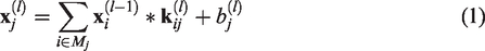
Traditional convolutional neural network consists of two stages: filtering stage (feature extraction stage) and classification stage. Generally, the feature extraction stage includes four layers: convolution layer, batch normalization (BN) layer, activation layer, and pooling layer. The classification stage is generally composed of multi-layer perceptron connections. For adapting to different tasks, many CNN structures have been proposed in previous research on fault diagnosis, such as TICNN, adversarial adaptive 1-D CNN (A2CNNs),²⁵ DNCNN, WDCNN, ACDIN, ICN, and so on, whose basic structural units are composed of the following neural network layers.

Convolutional layer

The convolution layer^26,27 convolves the local regions of input data with filter kernels, and each filter kernel uses the same weight to extract the local features of the input information and sharing the weight values

x_{j}^{(l)} = \sum_{i \in M_{j}} x_{i}^{(l - 1)} * k_{i j}^{(l)} + b_{j}^{(l)}

(1)where

M_{j}

is the current input characteristics, (l) denotes the convolution layer l,

x_{i}^{(l - 1)}

is input parameters taken from

M_{j}

, notation * denotes the convolution operation,

x_{j}^{(l)}

is the output in layer l, k is the weights of filter kernel, and b is bias.

Batch normalization

Batch normalization (BN) layer is designed to alleviate the problem of “gradient dispersion” in deep network, so that makes the training network model easier and more stable, and makes the convergence speed of the model accelerated.²⁸ Given the m-dimensional batch input x, the BN layer operates as follows

\begin{array}{l} {\hat{x}}^{(l)} = \frac{x^{(l)} - E [x^{(l)}]}{\sqrt{Var [x^{(l)}]}} \\ x_{B}^{^{(l)}} = γ {\hat{x}}^{(l)} + β \end{array}

(2)where

E [x^{(l)}]

is the expectation of input x,

Var [x^{(l)}]

is the variance of x, γ and β are the scale and shift parameters, respectively, and

x_{B}^{^{(l)}}

denotes the output after normalization.

Pooling layer and nonlinear activation function layer

Pooling is a downsampling operation, aiming at reducting the spatial size of the features and the parameters for the network, which has obvious effect on controlling over-fitting and improving model performance. Commonly, the max-pooling operation is described as follows

x_{j P}^{^{(l)}} = \max_{i \in W_{j}} {f (x_{i B}^{^{(l)}})}_{j}

(3)where

W_{j}

is pooling region of layer l,

x_{i B}^{^{(l)}}

the input after BN,

x_{j P}^{^{(l)}}

is the output after pooling, and f denotes nonlinear activation function, generally takes relu function.

As mentioned above, most of the neural networks designed in the field of fault diagnosis are based on the unit structure and its variants. Because of the flexibility of neural network design, such as the number of layers, structures, and so on, the diversity of neural network is caused. Therefore, how to select the accepted neural network as the basic structure for mechanical fault diagnosis research is a very important work, which is able to ensure the succession and reproducibility of the research, and then place deep learning at the service of the practical problems in the field of fault diagnosis. [Note that the citation “He et al.” has been changed to “Kaiming et al.” as per the reference list. If this is inaccurate, please update the citation and the reference.]In this paper, Resnet proposed by Kaiming et al.²⁴ is selected for reference, and some improvements are made to adapt to the research content of this paper. Resnet, known as an excellent neural network currently, has been applied widely to computer vision, natural language processing and other fields since it was proposed owing to its fine performance. Thus, it is reasonable to select Resnet. At the same time, it can avoid a lot of unnecessary network design work. The basic structure of Resnet shown in Figure 1 is residual learning unit, which consists of two 3 × 3 convolution networks connected in series, and the relationship between input X and output Y is as follows

Y = Φ (X, W_{i}) + X

(4)where Φ donates the residual mapping and W _i is the weight of each layer.

Figure 1.

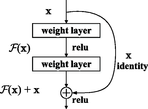
Residual learning unit.²⁴

The overall framework of proposed Resnet is shown in Figure 2. The input of CNN is the segment vibration signal of the bearing. The input layer passes the segment signal into the neural network and does not participate in the training. The down sampling layer consists of four continuous convolution layers, each of which has 16 small convolution kernels of 3 × 1 size. The first three convolution layers are followed by a normalization layer, respectively. We use C to denote the convolution layer and N to denote the normalization layer. The down sampling layer is followed by four consecutive Resnet blocks,²⁴ each of which consists of two residual modules as shown in Figure 1. Then, the average pooling layer is applied to down sample the features in residual learning. Finally, the features are flattened into a vector and input into a fully connection layer. The fault classification of training set signal is obtained by classifier.

Figure 2.

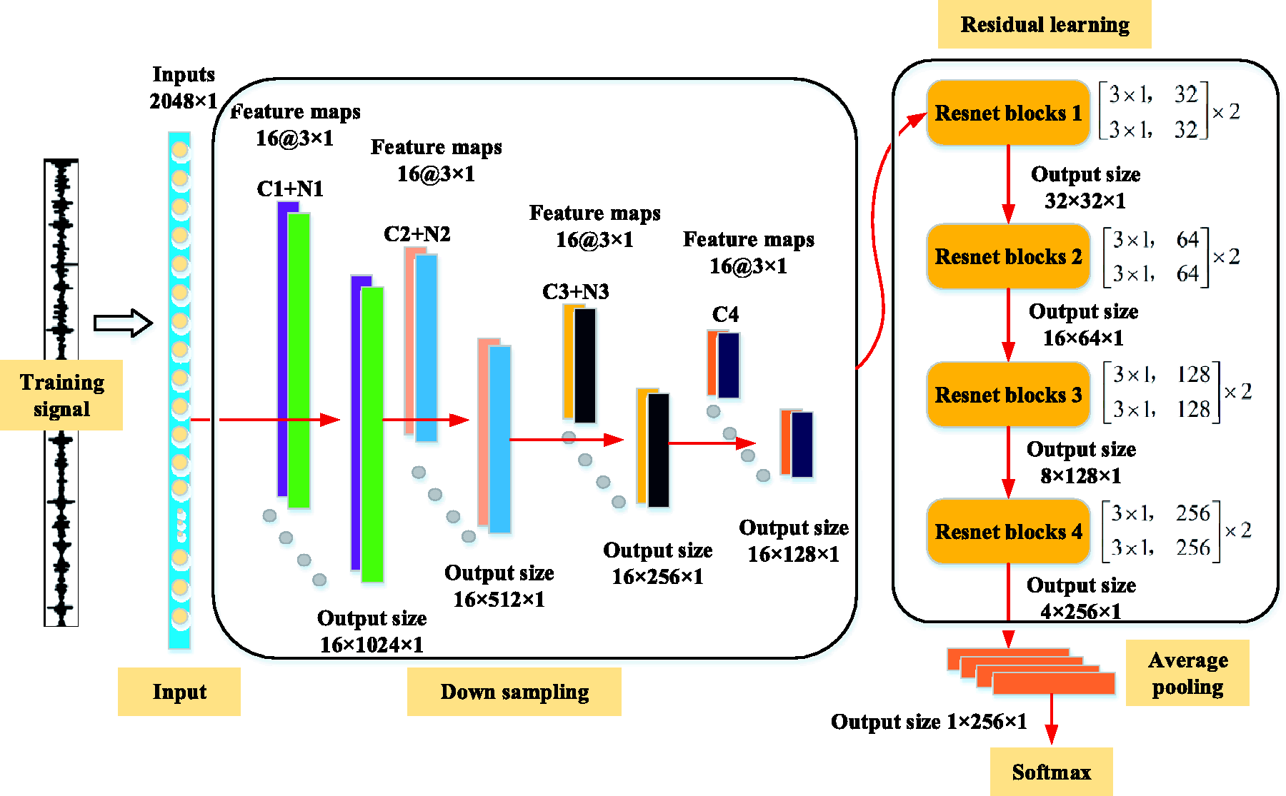
The architecture of Resnet1d.

Transfer learning based on maximum mean discrepancy

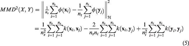
Maximum mean discrepancy (MMD) is the most frequently used measure in transfer learning, which measures the distance between two distributions in reproducing Hilbert space and is a kernel learning method. The formulation of MMD can be defined as

\begin{array}{l} M M D^{2} (X, Y) = {‖ \frac{1}{n_{s}} \sum_{i = 1}^{n_{s}} ϕ (x_{i}) - \frac{1}{n_{t}} \sum_{j = 1}^{n_{t}} ϕ (y_{j}) ‖}_{H}^{2} \\ = \frac{1}{n_{s}^{2}} \sum_{i = 1}^{n_{s}} \sum_{j = 1}^{n_{s}} k (x_{i}, x_{j}) - \frac{2}{n_{s} n_{t}} \sum_{i = 1}^{n_{s}} \sum_{j = 1}^{n_{t}} k (x_{i}, y_{j}) + \frac{1}{n_{t}^{2}} \sum_{i = 1}^{n_{t}} \sum_{j = 1}^{n_{t}} k (y_{i}, y_{j}) \end{array}

(5)where X and Y denote two datasets with a certain degree of similarity, n_s and n_t are the numbers of samples in the two datasets, respectively,

H

is a reproducing Hilbert space, and k(•) is a kernel function. The kernel type is selected from radial basis function (RBF) in this paper. In the method of this paper, MMD term is appended to the loss of Resnet1d for optimization as shown in Figure 3.

Figure 3.

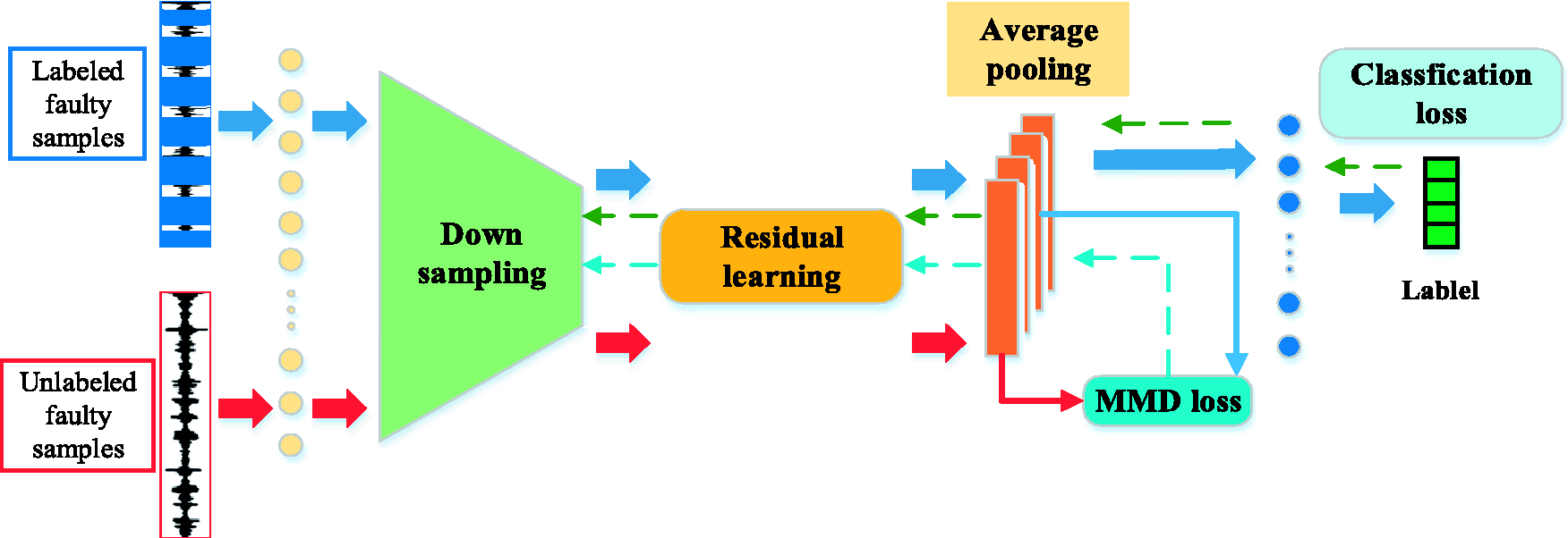
The architecture of Resnet1d with MMD for unlabeled fault diagnosis.

As shown in Figure 3, we can train the Resnet1d model on the labeled faulty samples generally. The classification loss is defined by cross-entropy between predict label and true label on the labeled faulty samples. Meanwhile, the unlabeled faulty data will be input into the network, which is used to calculate the MMD with the feature from labeled data, before the fully connection layer. When the model is trained, the error of back propagation consists of MMD loss and classification loss, which is written as

L (θ) = l_{c} + λ MMD (X_{labeled}, X_{unlabeled})

(6)where

θ

is the parameter of the model,

l_{c}

is the classification loss, and

λ

is non-negative parameter. In this paper, the learning rate of the model is set by using formula 0.001/(1 + 10 × p)^0.75, the

λ

is changed by using the formula 2/(1 + exp (–10 × p)) – 1, p is the training progress parameter,^29,30 and

X_{labeled}

and

X_{unlabeled}

are the learned transferable features from the last feature extraction layer.

The proposed model is trained by jointly minimizing two terms: (1) the error between the true labels and predicted labels of the source, which is the classification loss $l_{c}$ ; (2) the MMD of the learned transferable features after feature extraction layer. Thus, the model is finally trained by

\min_{θ} L (θ) = \min_{θ} [l_{c} + λ MMD (X_{labeled}, X_{unlabeled})]

(7)

By minimizing the $L (θ)$ , the mini-batch stochastic gradient descent (SGD) and backpropagation algorithm are used for optimization;²⁹ thus, the gradient of objective function is

\nabla_{θ} L (θ) = \frac{\partial l_{c}}{\partial θ} + λ \frac{\partial MMD (X_{labeled}, X_{unlabeled})}{\partial θ}

(8)

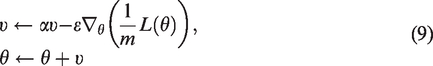
The update rules of SGD optimization algorithm are as follows

\begin{array}{l} υ \leftarrow α υ - ε \nabla_{θ} (\frac{1}{m} L (θ)), \\ θ \leftarrow θ + υ \end{array}

(9)where

α

is momentum parameters,

ε

is learning rate, m is a mini-batch m samples in training dataset, and

θ

is the parameter of the model.

Data description and experimental setup

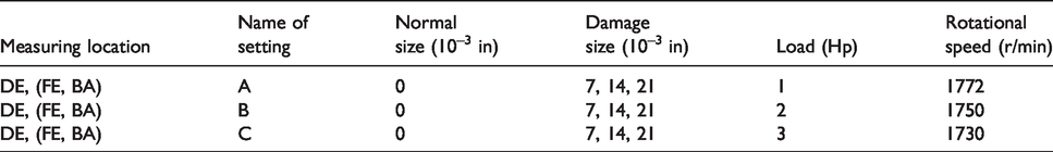
The original data comes from the open bearing data of Case Western Reserve University (CWRU),³⁰ which has been cited and studied by a large number of literatures. Three acceleration sensors are used to collect data from driving end, fan end, and base, respectively, at sampling frequencies of 12 and 48 kHz. There are four types of bearing fault: normal, ball fault, inner race fault, and outer race fault, containing 0.007, 0.014, and 0.021 in of fault diameter. The experiments are performed under four loads (0, 1, 2, and 3 hp). In the experiment, we select the data at 12 kHz sampling frequency and divide a total of 10 fault categories. The denotation of A, B, and C is utilized to represent the load of 1, 2, and 3 hp under 10 different fault conditions, respectively. The denotation of DE, FE, and BA is utilized to represent different measuring location. In particular, DE also denotes the faulty end; meanwhile, FE and BA denote non-fault location points. Details of tasks design are listed in Table 1.

Table 1.

Training and testing data from CWRU.

Measuring location	Name of setting	Damage size (10^–3 in)	Load (Hp)	Rotational speed (r/min)
DE, (FE, BA)	A	7, 14, 21	1	1772
DE, (FE, BA)	B	7, 14, 21	2	1750
DE, (FE, BA)	C	7, 14, 21	3	1730

For clarity, the denotation DE: A → B is utilized to represent the task from training dataset A (load 1) to testing dataset B (load 2) at driving end. The first goal is to test the method proposed in this paper for fault diagnosis performance under different operating conditions. In fact, the machine is always running under different conditions, and the model trained under one condition must be able to be applied to the diagnosis under another condition. For this purpose, six groups of different tasks are designed: DE: A → B, DE: B → A, DE: A → C, DE: C → A, DE: B → C, and DE: C → B.

The second goal is to use this method to study the fault diagnosis of bearings under different loads at non-fault ends. Because it is difficult to know the exact location of the fault in advance actually, the sensor is always arranged at the position away from the faulty end to collect data. For this purpose, some tasks are designed, i.e. FE: C → A and BA: C → A.

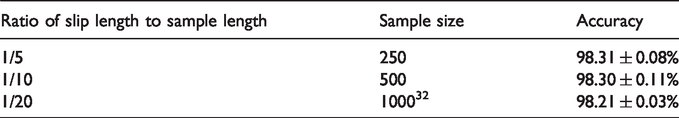
The time-shifting is a simple data augmentation technique to increase the number of training samples, that is, slicing the training time-domain signal with overlap.^13,14 In fact, Liu et al.³¹ have done some researches on the influence of time-shifting. The results show that the accuracy rate is still better for stationary signals, although the slip step is very small.³¹ However, the slip step needs to be optimized for nonstationary signal.³¹ In the paper, because of the input requirement of the neural network, the sample length is fixed to 2048. The result calculated by Resnet1d model is presented in Table 2. It can be seen from the table that the larger the slip step is, the smaller the sample size generated by data augment becomes. And there is little difference in accuracy. In some literature, the sample size is designed to be 1000.³² Considering the requirement of large data and the influence of computational complexity, the sample size of this paper is designed to be 500. The process is shown in Figure 4. The samples are prepared with time-shift and overlap from a long sequence.

Figure 4.

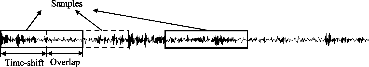
Data augment with time-shift and overlap.

Table 2.

The influence of the time-shifting.

Ratio of slip length to sample length	Sample size	Accuracy
1/5	250	98.31 ± 0.08%
1/10	500	98.30 ± 0.11%
1/20	1000³²	98.21 ± 0.03%

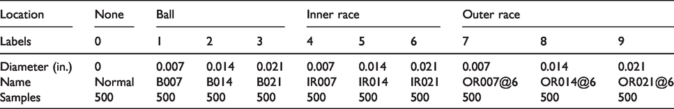
Ten types of faults are selected as research objects, and the corresponding labels are listed in Table 3.

Table 3.

Description of faulty types.

Location	None	Ball			Inner race			Outer race
Labels	0	1	2	3	4	5	6	7	8	9
Diameter (in.)	0	0.007	0.014	0.021	0.007	0.014	0.021	0.007	0.014	0.021
Name	Normal	B007	B014	B021	IR007	IR014	IR021	OR007@6	OR014@6	OR021@6
Samples	500	500	500	500	500	500	500	500	500	500

Results

Performance of Resnet1d under different working loads

As shown in Figure 5, SVM, TICNN, A2CNNs, ICN, Resnet1d, and Resnet1d with MMD (denoted as Rmmd) are compared at different tasks in experiment 1. Traditional machine learning algorithms SVM, performs poorly in domain adaptation, with average accuracy in the six tasks being around 61.37%. Some deep learning method proposed previously, i.e. TICNN, A2CNNs, and ICN perform better than traditional methods, with average accuracy being around 96.05, 94.46, and 97.16, respectively. In contrast, the proposed method Resnet1d gets much more precise than the other method, achieving 98.30% accuracy in average. It is proved that the deep learning method based on Resnet proposed in this paper can also solve the bearing fault diagnosis under different loads and even achieve higher accuracy. Finally, it can be seen from the figure that the Resnet1d with MMD method achieves higher accuracy than Resnet1d under each task. Thus, this also shows that the data collected from fault detection points contain sufficient feature information and are similar, which is beneficial to model learning.

Figure 5.

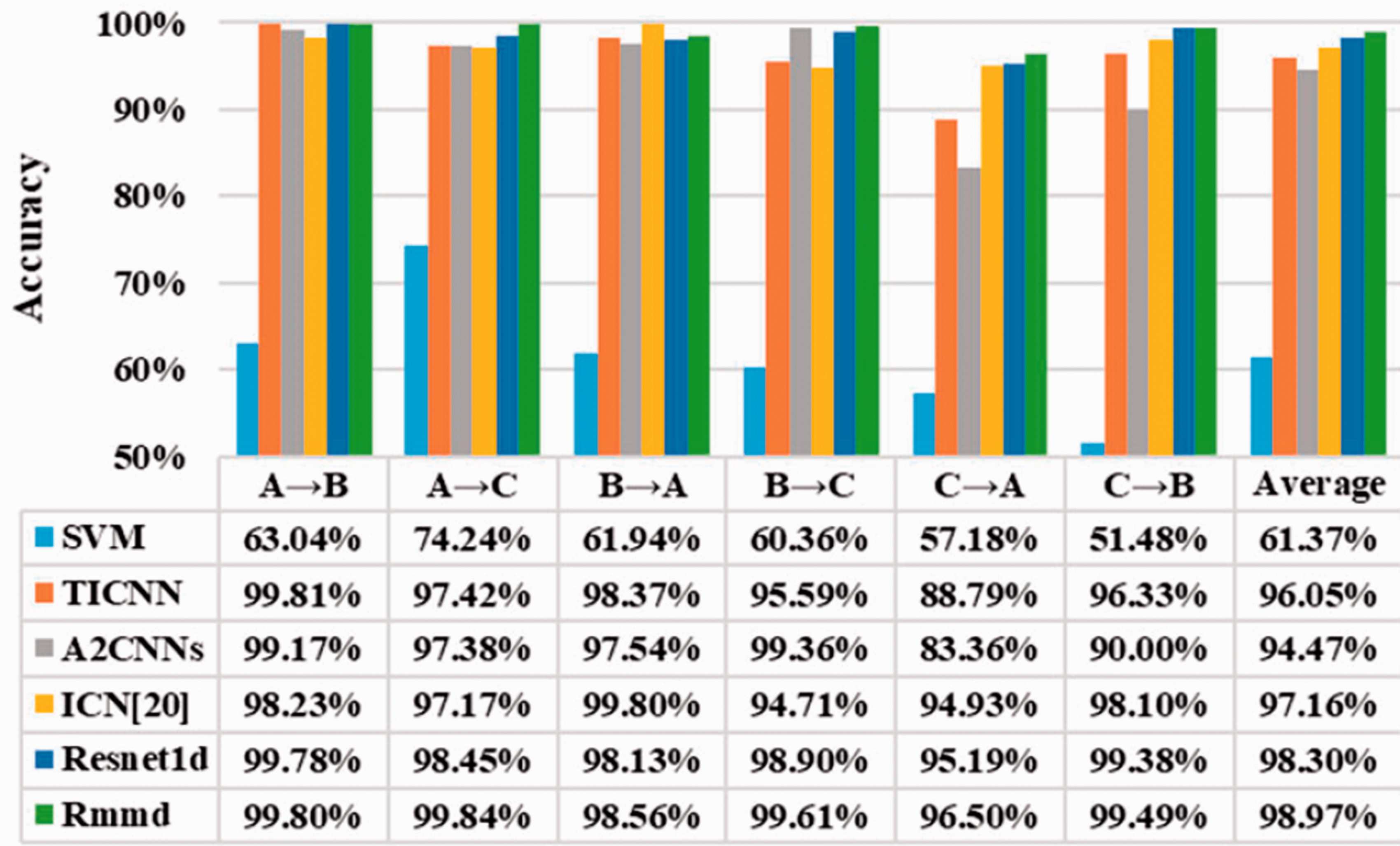
Comparison of the accuracy of different methods.

Performance of Resnet1d under different working loads with non-faulty measuring points

As shown in Figure 6, Resnet1d and Resnet1d with MMD (denoted as Rmmd) are compared at different measuring points. By using Resnet1d model and comparing the diagnostic results at different measuring points, it can be found that the average accuracy of the model is the highest at the driving end (near the fault source), reaching 98.97%. The average accuracy at the base is 81.31%, while the accuracy at the fan end away from the faulty source is 77.50%. This is because the fault signal attenuates in transmission, so the signal collected from the measuring point far away from the faulty end may be contaminated by background noise, which leads to the decline of the accuracy. By using transfer learning skills to improve the generalization ability of model (Resnet1d with MMD), we can find that the accuracy has been improved greatly under different working loads at driving end, base, and fan end. The average accuracy increased from 77.50, 81.31, and 97.97 to 91.46, 97.64, and 98.97%, respectively. Why Resnet1d with MMD can improve the accuracy of fault diagnosis under different working loads at different measuring points will be analyzed later.

Figure 6.

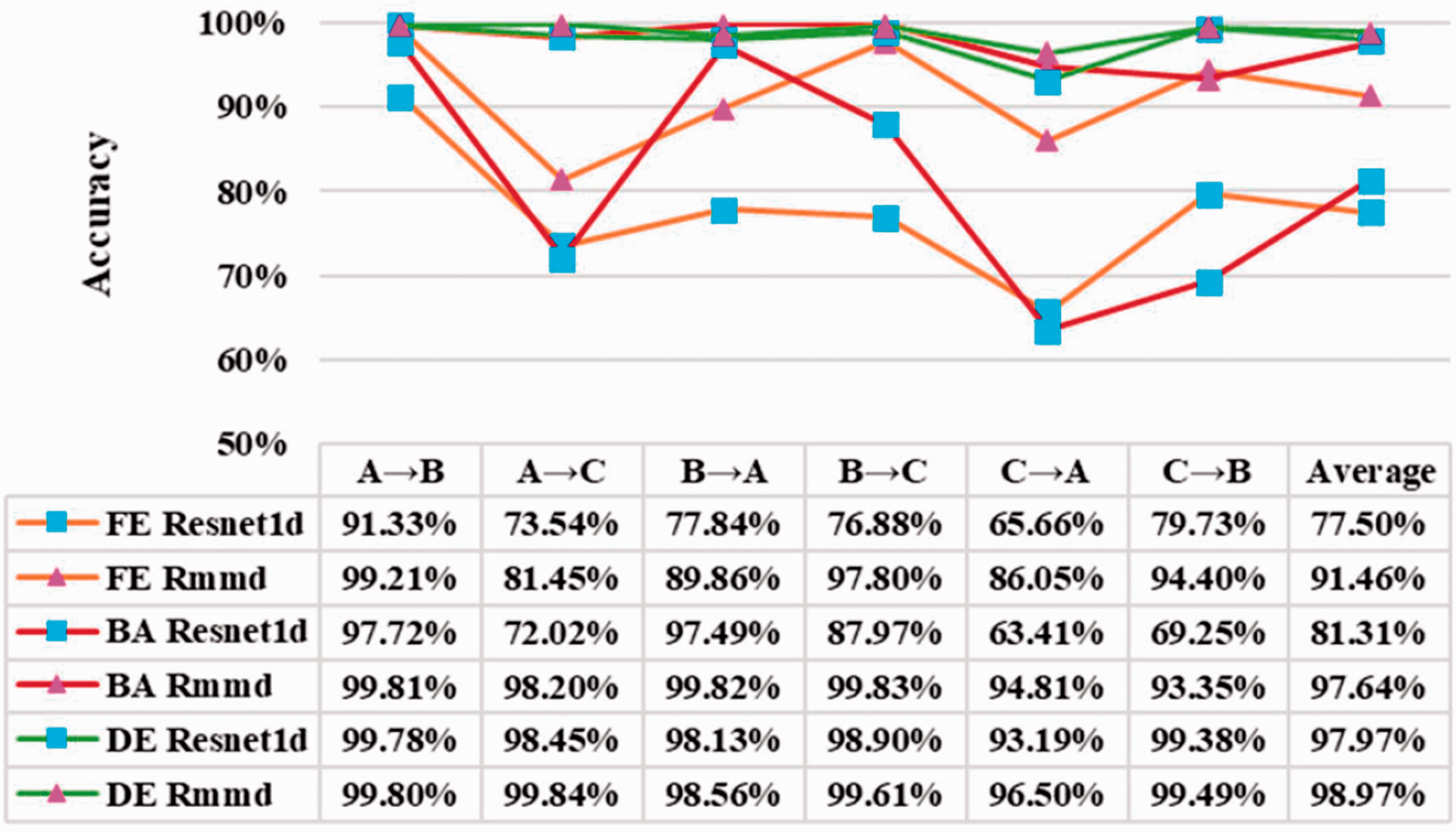
Comparison of the accuracy under different working loads and measuring points.

From Figure 6, it is also found that the accuracy of A → C and C → A is lower than that of other transfer tasks. Because the similarity of the signal data collected from the same fault form in two large-span working conditions is not high, it is difficult that the signal characteristics acquired under one condition is used for characterizing the signal characteristics under another condition. While the accuracy of A → C and C → A has been greatly improved by using Resnet with MMD model.

Network visualization

The results of feature extraction for different faults in the feature output layer of the neural network are shown in Figure 7. Red represents the neurons that are most activated, while white means the neurons are not activated. It can be seen from the figure that the distribution of the dark red is related to the distribution of the fault wave packet. Because the fault signal contains more periodic wave packets, the feature layer contains a large number of activated neurons. Compared with normal, we can see that the dark red areas of neurons are relatively less distributed.

Figure 7.

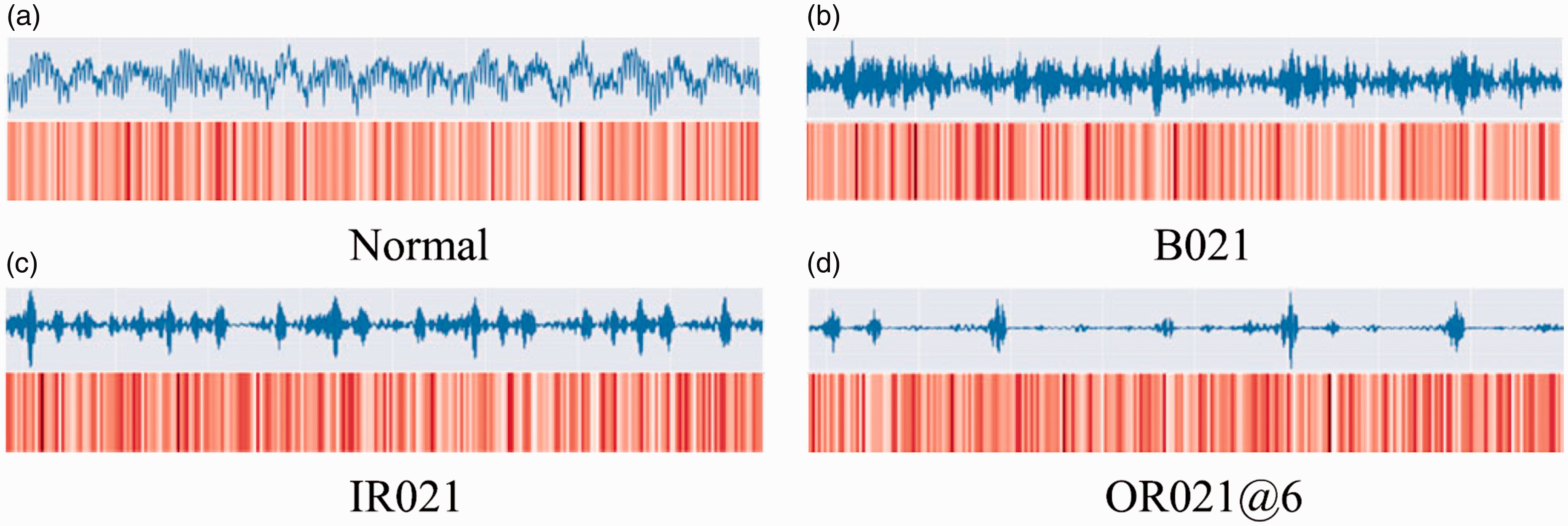
Network visualization in task DE: C → A at final feature extraction layer after pooling: (a) normal; (b) B021; (c) IR021; (d) OR021@6.

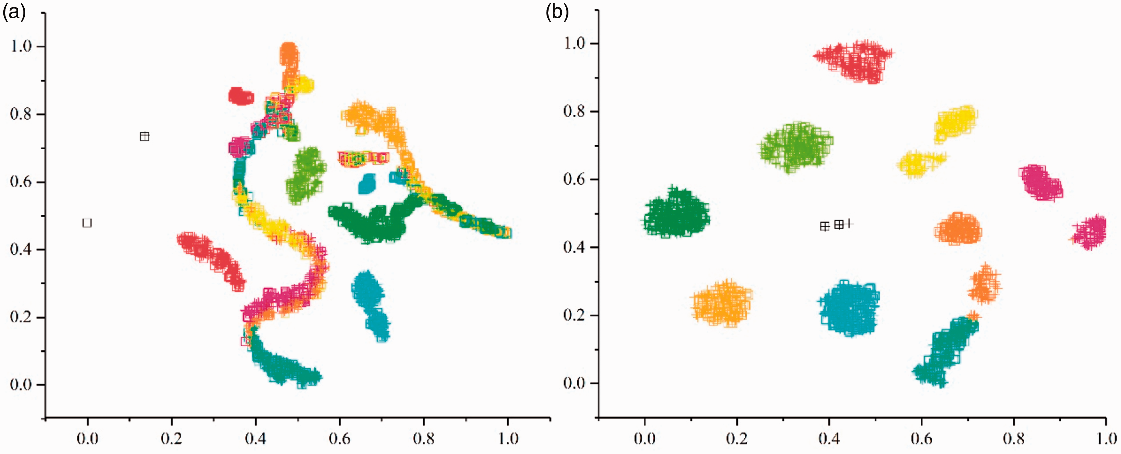
In order to fully understand the model proposed in this paper, the output of feature layer from the model is extracted for visual analysis. For this reason, the dimension reduction analysis method named t-SNE is adopted. And, we will take the case of C → A as an example to illustrate. Figures 8 to 10 show the dimension reduction results of the output data from feature layers at different measuring points, where □ denotes the dataset under load C and + denotes the dataset under load A.

From the results shown in Figure 8, most of the 10 categories of fault are well separated with two models, while the feature distribution of same label between load C and load A is aligned very well. It shows that the model trained by data that is acquired from the driver end (DE) near the faulty source gets higher diagnostic accuracy and better generalization performance.

Figure 8.

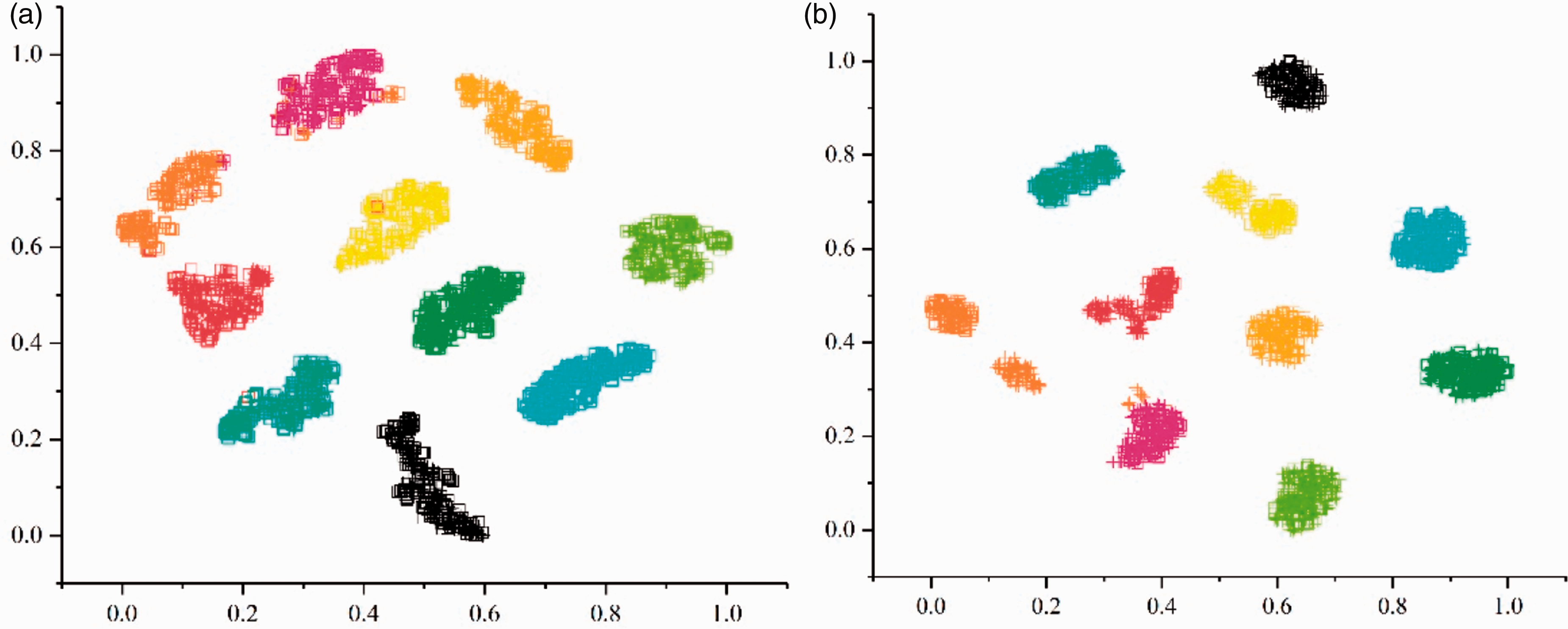
Network visualization in task DE: C → A: (a) Resnet1d; (b) Resnet1d with MMD.

Non-fault location point results are shown in Figures 9 and 10. It can be found that the data features learned by the Resnet1d model on the C dataset cannot characterize the A dataset. Although the fault categories can be separated, there are no longer similarity between C and A. Some categories have more overlapping areas, e.g. 7, 8, 9, while some categories have fewer overlapping areas, even errors, e.g. 2 and 3. This shows that the Resnet1d model trained by data collected from non-fault location points does not have good generalization performance. It should be added that the result of this misclassification is caused by the large differences between data sets and has nothing to do with the neural network itself. In order to improve the diagnostic accuracy, the parameter adjustment process of the neural network will be futile unless additional training data are added. Compared with Figure 10(a), it can be seen from Figure 10(b) that the generalization performance of the model has been greatly improved, not only can the categories be fully separated, but also the distribution of feature between the two datasets become similar. Therefore, compared with Resnet1d model, Resnet1d with MMD model can improve the bearing fault diagnosis accuracy of non-fault location points.

Figure 9.

Network visualization in task BA: C → A: (a) Resnet1d; (b) Resnet1d with MMD.

Figure 10.

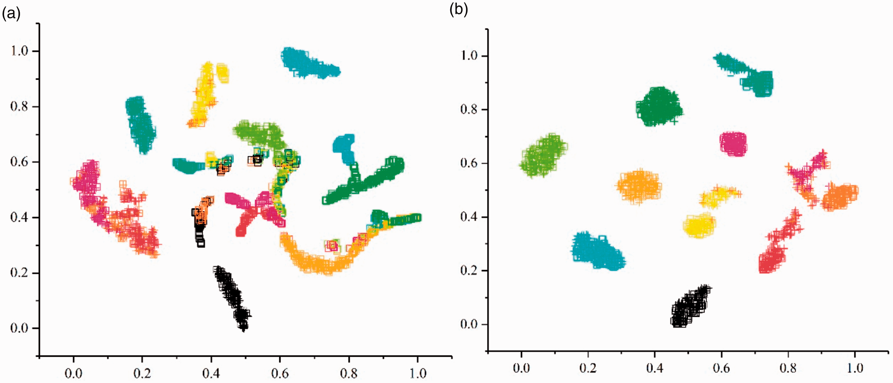
Network visualization in task FE: C → A: (a) Resnet1d; (b) Resnet1d with MMD.

Further analysis of the results of the transfer learning between the two conditions is given. Figure 11 shows the classification confusion matrix for each category in task A ↔ C. The categories 4–9 (categories 4, 5, and 6 correspond to inner race fault and categories 7, 8, and 9 correspond to outer race fault) at different measuring points can be identified and classified accurately. The diagnostic results of driving end and base show that negative migration occurs in category 3 (B021). However, the results in fan end show that categories 1, 2, and 3 (correspond to roller fault) task A ↔ C are confused with each other easily. Because of the large difference between categories 1, 2, and 3 under load A and C, it leads to the phenomenon of negative migration. Compared with Figures 11(d) to (f) and 12 (a) to (c), Resnet1d model can hardly independently identify roller fault and IR014 faults, while Resnet11d with MMD model can significantly improve the diagnosis results of that, resulting in the improvement of overall diagnostic accuracy.

Figure 11.

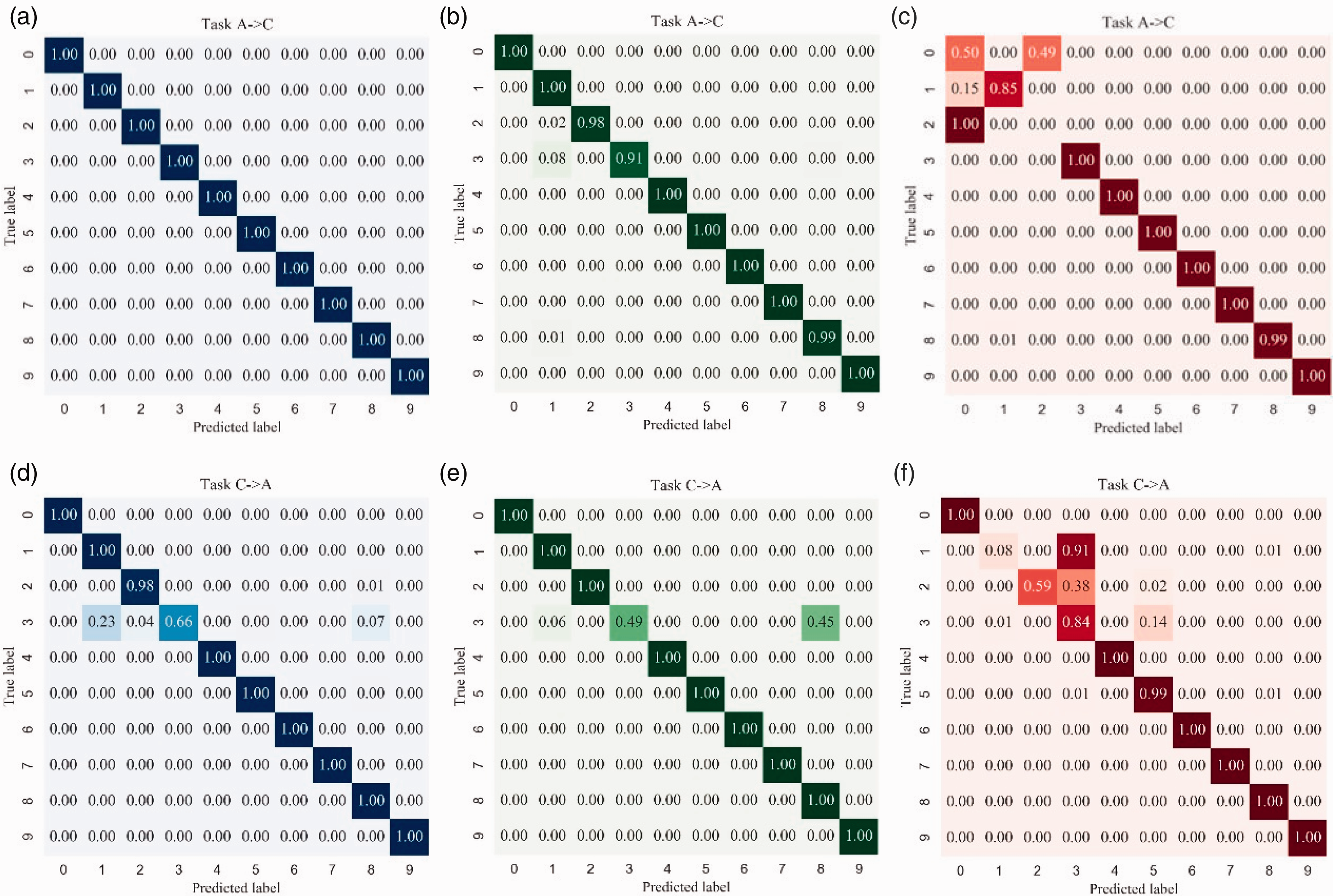
Normalized confusion matrixes in task A → C and task C → A calculated by Resnet1d with MMD: (a) DE; (b) BA; (c) FE; (d) DE; (e) BA; (f) FE.

Figure 12.

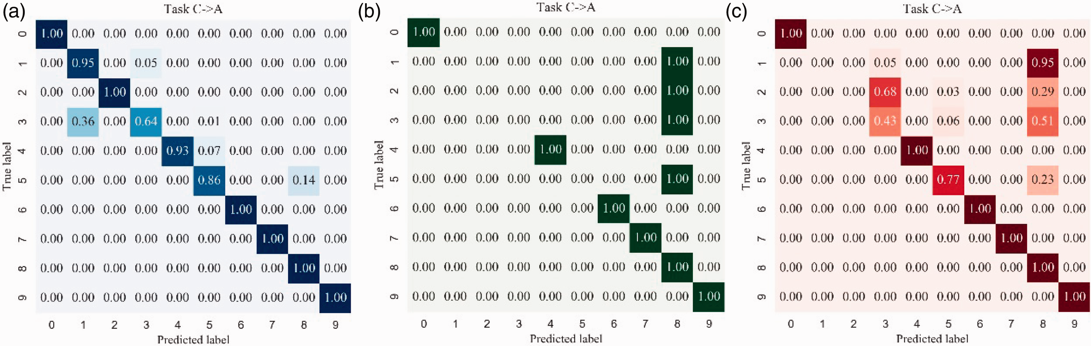
Normalized confusion matrixes in task C → A calculated by Resnet1d: (a) DE; (b) BA; (c) FE.

Conclusion

The application of intelligent diagnosis model in solving industrial practical problems is an important research topic. First, this paper designs a deep learning model based on the famous Resnet network, which reduces the randomness of model design. Second, using the idea of transfer learning, MMD is used to measure the distance between different data sets to improve the generalization performance of the model. Finally, the experiments of fault diagnosis and recognition under different loads and non-fault location points are designed, and the experimental results show that the proposed method performs well in the diagnosis of non-fault location points and bearings under different working loads. More future work can be carried out in the following two aspects: (1) testing real data; (2) considering the more realistic situation of category imbalance.

Footnotes

Declaration of conflicting interests

The author(s) declared no potential conflicts of interest with respect to the research, authorship, and/or publication of this article.

Funding

The author(s) disclosed receipt of the following financial support for the research, authorship, and/or publication of this article: This work was supported by the 111 Project P.R.China (Grant No. B16038).

ORCID iDs

Chongyu Wang

Di Zhang

References

Liang

, et al. Diagonal slice spectrum assisted optimal scale morphological filter for rolling element bearing fault diagnosis. Mech Syst Sig Process 2017; 85: 146–161.

Jiang

, et al. An improved EEMD with multi-wavelet packet for rotating machinery multi-fault diagnosis. Mech Syst Sig Process 2013; 36: 225–239.

Zhang

Zhou

JZ.

Multi-fault diagnosis for rolling element bearings based on ensemble empirical mode decomposition and optimized support vector machines. Mech Syst Sig Process 2013; 41: 127–140.

Peng

Tse, Peter

, et al. A comparison study of improved Hilbert–Huang transform and wavelet transform: application to fault diagnosis for rolling bearing. Mech Syst Sign Process 2005; 19: 974–988.

Yan

Gao Robert

Chen

, et al. Wavelets for fault diagnosis of rotary machines: a review with applications. Mech Syst Sign Process 2014; 96: 1–15.

Lei

Lin

, et al. A review on empirical mode decomposition in fault diagnosis of rotating machinery. Mech Syst Sign Process 2013; 35: 108–126.

Yau

H-T

, et al. Fractional-order chaotic self-synchronization based tracking faults diagnosis of ball bearing systems. IEEE Trans Ind Electron 2016; 63: 3824–3833.

Kuo

Hsieh Yau

H-T

, et al. Research and development of a chaotic signal synchronization error dynamics-based ball bearing fault diagnostor. Entropy 2014; 16: 5358–5376.

Yau

H-T

, et al. Ball bearing test-rig research and fault diagnosis investigation. IET Sci Measure Technol 2016; 10: 259–265.

10.

Bengio

Hinton

Deep learning. Nature 2015; 521: 436–444.

11.

Socher

Huval

Bath

, et al. Convolutional-recursive deep learning for 3D object classification. NIPS 2012; 665–673.

12.

Gan

Wang

, et al. Construction of hierarchical diagnosis network based on deep learning and its application in the fault pattern recognition of rolling element bearings. Mech Syst Sign Process 2016; 72: 92–104.

13.

Wei

Gaoliang

Chuanhao

, et al. A new deep learning model for fault diagnosis with good anti-noise and domain adaptation ability on raw vibration signals. Sensors 2017; 17: 425.

14.

Zhang

Peng

, et al. A deep convolutional neural network with new training methods for bearing fault diagnosis under noisy environment and different working load. Mech Syst Sign Process 2018; 100: 439–453.

15.

Shao

Jiang

Zhang

, et al. Rolling bearing fault feature learning using improved convolutional deep belief network with compressed sensing. Mech Syst Sign Process 2018; 100: 743–765.

16.

Feng

, et al. Deep normalized convolutional neural network for imbalanced fault classification of machinery and its understanding via visualization. Mech Syst Sign Process 2018; 110: 349–367.

17.

Pan

Chen

, et al. LiftingNet: a novel deep learning network with layerwise feature learning from noisy mechanical data for fault classification. IEEE Trans Ind Electron 2017; 65: 4973–4982.

18.

Szegedy

Liu

Jiayang

, et al. Going deeper with convolutions. In: Proceedings of the IEEE conference on computer vision and pattern recognition, Boston, MA, USA, 1–9 June 2015.

19.

Chen

Peng

Xie

, et al. ACDIN: bridging the gap between artificial and real bearing damages for bearing fault diagnosis. Neurocomputing 2018; 294: 61–71.

20.

Zhi

Peng

Chen

, et al. A convolutional neural network based on a capsule network with strong generalization for bearing fault diagnosis. Neurocomputing 2019; 323: 62–75.

21.

Christian

Kimotho

, et al. Condition monitoring of bearing damage in electromechanical drive systems by using motor current signals of electric motors: a benchmark data set for data-driven classification. In: European conference of the prognostics and health management society, Bilbao, Spain, July 2016.

22.

Alex

Ilya

Hinton

GE.

ImageNet classification with deep convolutional neural networks. In: Proceeding NIPS'12 proceedings of the 25th international conference on neural information processing systems, Lake Tahoe, Nevada, 1097–1105, December 2012.

23.

Simonyan

Zisserman

Very deep convolutional networks for large-scale image recognition, https://arxiv.org/abs/1409.1556 (accessed 4 September 2014).

24.

Kaiming

Xiangyu

Shaoqing

, et al. In: Proceedings of the IEEE conference on computer vision and pattern recognition, Las Vegas, NV, USA, June 2016, pp.770–778.

25.

Zhang

Hao

, et al. Adversarial adaptive 1-D convolutional neural networks for bearing fault diagnosis under varying working condition, https://arxiv.org/abs/1805.00778 (accessed 1 May 2018).

26.

LeCun

Boser

Denker

, et al. Backpropagation applied to handwritten zip code recognition. Neural Comput 1989; 1: 541–551.

27.

Weining

Bin

, et al. Deep model based domain adaptation for fault diagnosis. IEEE Trans Ind Electron 2016; 64: 2296–2305.

28.

Sergey

Christian

Batch normalization: accelerating deep network training by reducing internal covariate shift. In: Proceeding ICML'15 proceedings of the 32nd international conference on international conference on machine learning, Lille, France, July 2015, pp.448–456.

29.

Bottou

Online algorithms and stochastic approximations. In: Saad D (ed) Online learning and neural networks. Cambridge, UK: Cambridge University Press, 1998.

30.

Xinsheng

Loparo

KA.

Bearing fault diagnosis based on wavelet transform and fuzzy inference. Mech Syst Sign Process 2004; 18: 1077–1095.

31.

Liu

Meng

Chen

, et al. Dislocated time series convolutional neural architecture: an intelligent fault diagnosis approach for electric machine. IEEE Trans Ind Inf 2017; 13: 1310–1320.

32.

Wen

Gao

XY.

A new deep transfer learning based on sparse auto-encoder for fault diagnosis. IEEE Trans Syst Man Cybern Syst 2019; 49: 136–144.

33.

Ganin

Ustinova

, et al. Domain-adversarial training of neural networks. J Mach Learn Res 2016; 17: 1–35.

Deep learning for bearing fault diagnosis under different working loads and non-fault location point

Abstract

Keywords

Introduction

Related works

Convolutional layer

Batch normalization

Pooling layer and nonlinear activation function layer

Transfer learning based on maximum mean discrepancy

Data description and experimental setup

Results

Performance of Resnet1d under different working loads

Performance of Resnet1d under different working loads with non-faulty measuring points

Network visualization

Conclusion

Footnotes

Declaration of conflicting interests

Funding

ORCID iDs

References