Nonlinear optimal-based vibration control for systems with MR tuned vibration absorbers

Abstract

In this paper, the author proposes several approaches to nonlinear optimal-based control implementation. The vibrating system (structure) equipped with two tuned vibration absorbers (TVAs) is analysed against a system with one TVA. For control purposes, MR dampers are used instead of TVAs' passive viscous dampers. The main contribution of this research is the development and numerical verification of three nonlinear optimal-based vibration control concepts (the implementation of one-step optimal control, quasi-optimal control, and the optimal-based modified ground-hook law) that produce MR damper required current (not required force) as their output (thus force tracking algorithm that results in control inaccuracy is entirely omitted here), and that may be directly applicable for online and real-time control; moreover, all of the MR damper force constraints (no active forces; lower and upper limits; nonlinear, hysteresis-type dynamics) are embedded in the control technique, thus the solution is optimal for the assumed actuator respecting its limitations. The proposed approaches are investigated against the standard ground-hook law and passive TVA(s) with optimally tuned (i.e. having a frequency response maxima of equal and lowest values) parameters. The performance of all the solutions for the one- and two-TVA systems is compared, confirming the validity and efficiency of the three proposed concepts: almost 50% reduction of the Dynamic Amplification Factor is possible with regard to the respective optimally tuned passive 1 TVA and 2 TVA configurations. No offline calculation, excitations/disturbances assumption, or frequency determination is necessary.

Introduction

Vibration may lead to both damage and fatigue wear, which may be the problem of the systems and structures with intrinsic elasticity. Slender, beam-type structures such as towers, masts, chimneys, wind turbines,^1–7 bridges,^8,9 high buildings^10,11 as well as plate structures^12,13 etc. usually have small modal damping ratios and can suffer excessive (and dangerous) resonant vibrations. For many systems, vibration is an undesirable behaviour. Thus many structures and systems are equipped with vibration attenuation solutions. The concepts utilised to reduce vibration include tuned vibration absorbers (TVAs), tuned liquid (column) dampers, viscoelastic/hydraulic dampers, granular dampers, piezoelectric actuators, etc.^14,15 Passive, semiactive, and active TVAs are widely spread vibration reduction solutions for vibrating systems/slender structures (towers, high buildings, bridges, chimneys, etc.). In the standard (passive) approach, TVA consists of the additional moving mass, spring and viscous damper, which parameters are tuned to the selected (most often first) mode of the vibration. ¹⁶ Passive TVAs work well at the load conditions characterised with a single frequency to which they are tuned but cannot adapt to a wide excitation spectrum. In real world conditions, the frequency response of many systems/structures may vary (more, if the damping is low), thus more advanced TVA solutions are regarded to tune the TVA operating frequency. Among them, magnetorheological (MR) TVAs are placed,^5,6,11,17 as using an MR damper (instead of a viscous damper) guarantees a wide range of resistance force and fast response times, and high operational robustness along with minor energy requirements as compared with the active systems.^1,18–24 As simulations and experiments show, the implementation of the MR damper in a TVA system may lead to further vibration reduction in relation with the passive TVA.^5,6 The concept presented in this paper was originally developed for the vibration attenuation of slender structures, namely wind turbine tower-nacelle system, using its scaled model.^25–28 The first bending mode of the structure is analysed only, and the MR TVA(s) is (are) tuned to its frequency.

Most of the MR damper (including MR TVA) online and real-time control algorithms are based on the bang-bang approach (e.g. the two-level sky hook or ground hook concepts), ²⁹ fuzzy logic^30,31 or, most widely, two-stage concepts with the calculation of the MR damper required force using the original Den Hartog approach, adaptive (positive or negative) stiffness/damping/friction, LQR/LQG, etc., being the first stage, and the MR damper force tracking algorithms using the feed-forward loop with the MR damper forward or inverse model, and the feedback loop with damper force sensor signal and, e.g., PI control algorithm.^{18,20,32–36} The two-stage approaches suffer from an inability to produce the required (by the first stage algorithm) MR damper force pattern due to the impossibility to generate active forces, and force value limitations: lower constraint imposed by the residual force at zero current, and upper constraint imposed by the piston velocity and maximum current that can be fed through the MR damper coil. As a result, the force pattern, often carefully determined at the first stage, is not the same at the output of the second stage thus vibration control results are compromised. Another problem is that such advanced and sophisticated first-stage algorithms need oscillation frequency determination which may be an issue for polyperiodic (e.g. transient, coupled vibration phases) or random (e.g. seismic) excitations – for such situations, these algorithms switch to the passive operation mode.

In the present research, the author proposes an entirely different concept: all of the MR damper force constraints (the inability to generate active forces along with both lower and upper force value limitations as well as nonlinear, hysteresis-type MR damper dynamics) are an intrinsic part of the control method, adopting the nonlinear control techniques. Throughout them, one may distinguish the optimal, maximum principle-based methods^4,13,37 with the receding horizon control/model predictive control, ³⁸ the control Lyapunov function-based methods ⁸ including (adaptive) sliding mode control and backstepping,^10,39–42 (feedback) linearisation methods with linear optimal control theory based on the Riccati equation solution, ¹⁰ the approximating sequence of Riccati equations, ⁴³ etc. Each of the method groups has its advantages and disadvantages, e.g. the first method group is performance (or arbitrary quality criteria minimisation) oriented with the relatively high computational burden necessary for online and real-time implementation. The second group is stabilisation oriented and requires existence/knowing of the Lyapunov function, while the linearisation and approximation approaches often have their own problems with precise online or real-time mapping of nonlinear dynamics. Moreover, most of the proposed solutions are hardly applicable online, alternatively applicable for control-affine nonlinear systems or non-implicit control-state relations, whereas this is not always the case, as in the present problem.

In view of this, the analytical and numerical methods for nonlinear vibration that may be implemented online are widely searched for. The drawback of the classical Hamilton principle based methods is that for most of the real-life physical problems, it is impossible to prescribe terminal conditions. Hence, He^44,45 proposed the modified Hamilton principle for initial value problems with acceptable accuracy considering the simple solution procedure. He gave strict derivation, first deduced in the history, valid for all initial-value problems, important in both pure and applied sciences due to the complete elimination of the long-existing shortcomings in Hamilton’s principle. The natural final conditions satisfy automatically the physical requirements, making a vital innovation of Hamilton’s principle.

The current research’s main contribution is another approach to this issue. The paper covers the development and numerical verification of nonlinear-system-specific (regarding systems/structures equipped with single or multiple MR TVAs), maximum principle-based control solutions (one-step optimal control, quasi-optimal control, and optimal-based control including the modified ground-hook law) that are directly applicable for online and real-time implementation. They produce MR damper required current (not required force) as their output, thus a force tracking algorithm that always results in control inaccuracy is entirely omitted here. Furthermore, all of the MR damper force constraints are embedded in the control technique, thus the solution is optimal (quasi optimal or optimal based) for the assumed actuator, respecting its limitations. These approaches are investigated against the standard ground-hook law and passive TVA(s) with optimally tuned (i.e. having a frequency response maxima of equal and lowest values) parameters. The efficiency of all the solutions for the one- and two-TVA systems is compared, confirming the validity and advantages of the proposed concepts.

The paper is organised as follows. In the second section, the nonlinear optimal control concept using the maximum principle is introduced. Then, the vibration control problem with MR TVAs is formulated and solved using the Hamiltonian maximisation. The following sections describe the baseline implementation technique along with some alternative approaches, among which the modified ground-hook law is derived. This is expanded by the simulations results and several conclusions.

Nonlinear optimal control – the maximum principle

Assume state equation of the regarded system

$$\dot{\mathit{z}}\left(t\right)=\mathit{f}\left(\mathit{z}\left(t\right),\mathit{u}\left(t\right),t\right),t\in \left[t_0,t_1\right]$$

(1)where $\mathit{z}\left(t\right)$ is the state vector with the initial value $\mathit{z}\left(t_0\right)={\mathit{z}}_0$ , $\mathit{u}\left(t\right)$ is piecewise-continuous control vector with constraints, $u\left(t\right)\in U$ , and the quality index to be minimised is

$$G\left(\mathit{z},\mathit{u}\right)={\displaystyle {\int }_{t_0}^{t_1}g\left(\mathit{z}\left(t\right),\mathit{u}\left(t\right),t\right)\text{d}t}$$

(2)

Functions $f$ and $g$ are assumed to be continuously differentiable with respect to the state and continuous with respect to time and control. Let us define Hamiltonian in the form

$$H\left(\mathit{\xi }\left(t\right),\mathit{z}\left(t\right),\mathit{u}\left(t\right),t\right)=-g\left(\mathit{z}\left(t\right),\mathit{u}\left(t\right),t\right)+{\mathit{\xi }}^T\left(t\right)\mathit{f}\left(\mathit{z}\left(t\right),\mathit{u}\left(t\right),t\right)$$

(3)

If $\left({\mathit{z}}^{\text{*}}\left(t\right),{\mathit{u}}^{\text{*}}\left(t\right)\right)$ is an optimal controlled process (optimal trajectory of state and optimal control, respectively), there exist an adjoint (co-state) variable $\mathit{\xi }$   satisfying the equation (  ${\mathit{f}}_z$ and $g_z$ are $\mathit{f}$ and $g$ derivatives with respect to the state $\mathit{z}$ )

$$\dot{\xi }\left(t\right)=-{\mathit{f}}_z^{\text{*}T}\left({\mathit{z}}^{\text{*}}\left(t\right),{\mathit{u}}^{\text{*}}\left(t\right),t\right)\mathit{\xi }\left(t\right)+g_z^T\left({\mathit{z}}^{\text{*}}\left(t\right),{\mathit{u}}^{\text{*}}\left(t\right),t\right),t\in \left[t_0,t_1\right]$$

(4)with a terminal (transversality) condition

$$\mathit{\xi }\left(t_1\right)=\mathbf{0}$$

(5)so that ${\mathit{u}}^{\text{*}}\left(t\right)$ maximises the Hamiltonian over the set $U$ for almost all $t\in \left[t_0,t_1\right]$ , ⁴⁶ i.e.

$${\mathit{u}}^{\text{*}}\left(t\right)=\arg \underset{\mathit{u}\left(t\right)\in U}{\max }H\left(\mathit{\xi }\left(t\right),{\mathit{z}}^{\text{*}}\left(t\right),\mathit{u}\left(t\right),t\right)$$

thus

$$H\left(\mathit{\xi }\left(t\right),{\mathit{z}}^{\text{*}}\left(t\right),{\mathit{u}}^{\text{*}}\left(t\right),t\right)\ge H\left(\mathit{\xi }\left(t\right),{\mathit{z}}^{\text{*}}\left(t\right),\mathit{u}\left(t\right),t\right)\forall \mathit{u}\left(t\right)\in U$$

(6)

Problem formulation

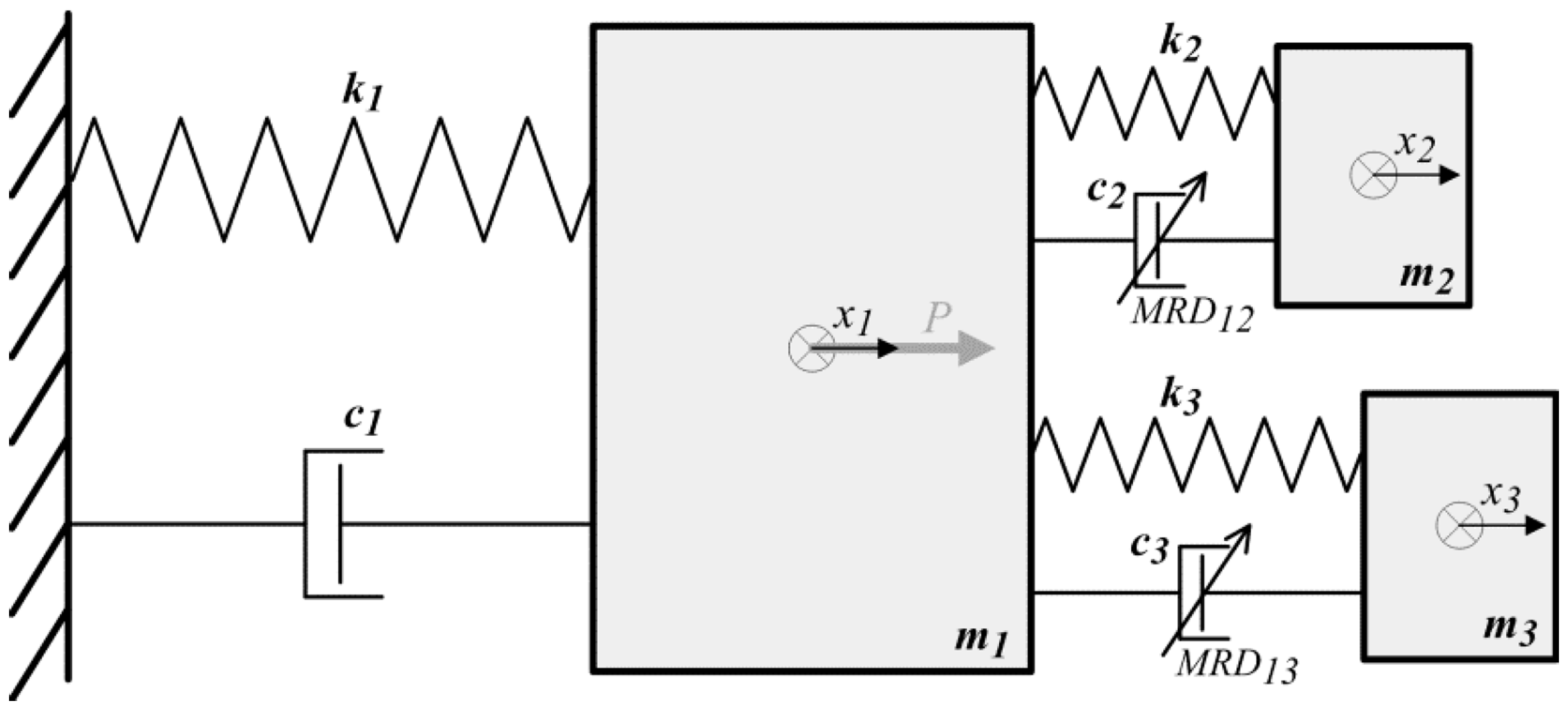
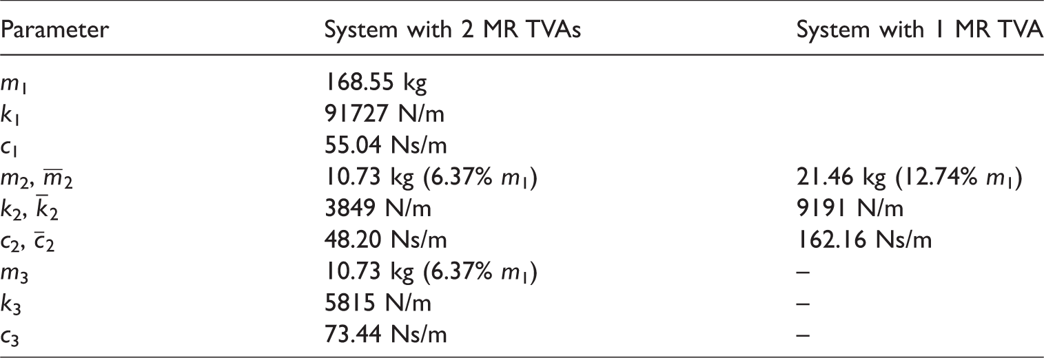
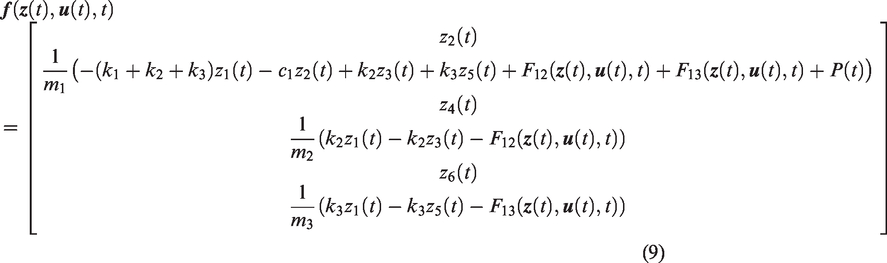
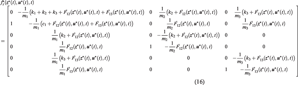
In general, we assume a primary vibrating system (structure) of (modal) mass m₁, (modal) stiffness k₁ and (modal) damping c₁, and two TVAs of mass m₂, m₃, stiffness k₂, k₃, and damping c₂, c₃, respectively – see Figure 1. The movement of all m₁, m₂, and m₃ is restricted to be linear displacement x₁(t), x₂(t), and x₃(t), respectively, along the axis (horizontal in Figure 1) of the applied excitation force $P\left(\text{t}\right)$ . The masses m₂, m₃ are assumed to be 6.37% of the mass m₁ each, as the 5 ÷ 10% mass ratio range is regarded as optimal concerning the efficiency to the added mass ratio. The parameters k₂, k₃, c₂, c₃ are tuned to obtain three maxima of x₁(t) amplitude output frequency response function of the lowest (for the assumed m₂ and m₃) and equal values. For control purposes, passive damping c₂ and c₃ is replaced by the MR dampers MRD₁₂ and MRD₁₃ of RD1097-1 series. ²¹ Such configurations are further compared with the baseline primary system equipped with single TVA of mass

Figure 1.

Diagram of the regarded system with two MR TVAs.

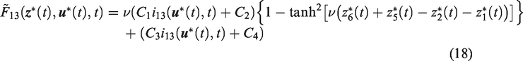
${\overline{m}}_2$ = m₂ + m₃ = 2m₂, with stiffness ${\overline{k}}_2$ and damping ${\overline{c}}_2$ parameters tuned according to the standard Den Hartog approach. ¹⁶ For control purposes, again passive damping ${\overline{c}}_2$ is replaced by the (assumptive) MR damper ${\overline{MRD}}_{12}$ of the doubled RD1097-1 force. The values of the adopted system parameters are presented in Table 1.

Table 1.

System parameters.

Parameter	System with 2 MR TVAs	System with 1 MR TVA
m 1	168.55 kg
k 1	91727 N/m
c 1	55.04 Ns/m
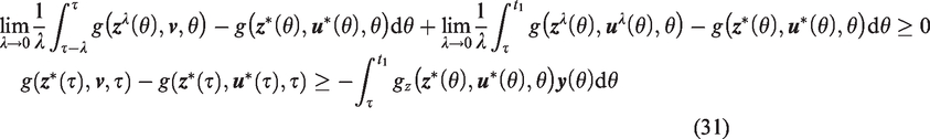
m2, ${\overline{m}}_2$	10.73 kg (6.37% m1)	21.46 kg (12.74% m1)
k2, ${\overline{k}}_2$	3849 N/m	9191 N/m
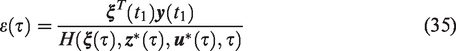
c2, ${\overline{c}}_2$	48.20 Ns/m	162.16 Ns/m
m 3	10.73 kg (6.37% m1)	–
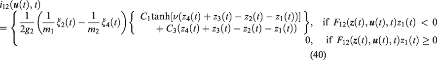
k 3	5815 N/m	–
c 3	73.44 Ns/m	–

Let us assume the state (7) and the control (8) vector in the form

$$\mathit{z}\left(t\right)={\left[\begin{array}{ccc}\begin{array}{cc}{z}_1\left(t\right)& z_2\left(t\right)\end{array}& \begin{array}{cc}{z}_3\left(t\right)& z_4\left(t\right)\end{array}& \begin{array}{cc}{z}_5\left(t\right)& z_6\left(t\right)\end{array}\end{array}\right]}^T$$

(7)

$$\mathit{u}\left(t\right)={\left[\begin{array}{cc}{u}_{12}\left(t\right)& u_{13}\left(t\right)\end{array}\right]}^T$$

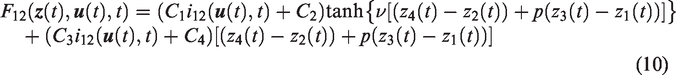
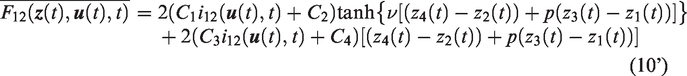
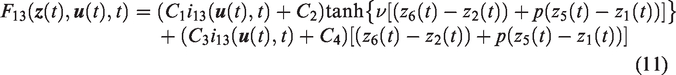
(8)where $z_1\left(t\right)=x_1\left(t\right)$ , $z_2\left(t\right)={\dot{x}}_1\left(t\right)$ , $z_3\left(t\right)=x_2\left(t\right)$ , $z_4\left(t\right)={\dot{x}}_2\left(t\right)$ , $z_5\left(t\right)=x_3\left(t\right)$ , $z_6\left(t\right)={\dot{x}}_3\left(t\right)$ . The right-hand side of (1) is

$$\begin{array}{l}\mathit{f}\left(\mathit{z}\left(t\right),\mathit{u}\left(t\right),t\right)\\ =\left[\begin{array}{c}\begin{array}{c}{z}_2\left(t\right)\\ \frac{1}{m_1}\left(-\left(k_1+k_2+k_3\right)z_1\left(t\right)-c_1{z}_2\left(t\right)+k_2{z}_3\left(t\right)+k_3{z}_5\left(t\right)+F_{12}\left(\mathit{z}\left(t\right),\mathit{u}\left(t\right),t\right)+F_{13}\left(\mathit{z}\left(t\right),\mathit{u}\left(t\right),t\right)+P\left(t\right)\right)\end{array}\\ \begin{array}{c}{z}_4\left(t\right)\\ \frac{1}{m_2}\left(k_2{z}_1\left(t\right)-k_2{z}_3\left(t\right)-F_{12}\left(\mathit{z}\left(t\right),\mathit{u}\left(t\right),t\right)\right)\end{array}\\ \begin{array}{c}{z}_6\left(t\right)\\ \frac{1}{m_3}\left(k_3{z}_1\left(t\right)-k_3{z}_5\left(t\right)-F_{13}\left(\mathit{z}\left(t\right),\mathit{u}\left(t\right),t\right)\right)\end{array}\end{array}\right]\end{array}$$

(9)where

$$\begin{array}{l}{F}_{12}(\mathit{z}\left(t\right),\mathit{u}\left(t\right),t)=(C_1{i}_{12}(\mathit{u}\left(t\right),t)+C_2)\tanh \left\{\nu [(z_4\left(t\right)-z_2\left(t\right))+p(z_3\left(t\right)-z_1\left(t\right))]\right\}\\ +(C_3{i}_{12}(\mathit{u}\left(t\right),t)+C_4)[(z_4\left(t\right)-z_2\left(t\right))+p(z_3\left(t\right)-z_1\left(t\right))]\end{array}$$

(10)

$$\begin{array}{l}\overline{F_{12}\left(\mathit{z}\left(t\right),\mathit{u}\left(t\right),t\right)}=2\left(C_1{i}_{12}\left(\mathit{u}\left(t\right),t\right)+C_2\right)\tanh \left\{\nu \left[\left(z_4\left(t\right)-z_2\left(t\right)\right)+p\left(z_3\left(t\right)-z_1\left(t\right)\right)\right]\right\}\\ +2\left(C_3{i}_{12}\left(\mathit{u}\left(t\right),t\right)+C_4\right)\left[\left(z_4\left(t\right)-z_2\left(t\right)\right)+p\left(z_3\left(t\right)-z_1\left(t\right)\right)\right]\end{array}$$

(10')and

$$\begin{array}{l}{F}_{13}\left(\mathit{z}\left(t\right),\mathit{u}\left(t\right),t\right)=\left(C_1{i}_{13}\left(\mathit{u}\left(t\right),t\right)+C_2\right)\tanh \left\{\nu \left[\left(z_6\left(t\right)-z_2\left(t\right)\right)+p\left(z_5\left(t\right)-z_1\left(t\right)\right)\right]\right\}\\ +\left(C_3{i}_{13}\left(\mathit{u}\left(t\right),t\right)+C_4\right)\left[\left(z_6\left(t\right)-z_2\left(t\right)\right)+p\left(z_5\left(t\right)-z_1\left(t\right)\right)\right]\end{array}$$

(11)are the MR damper resistance forces according to the hyperbolic tangent model, which parameters $C_1$ , $C_2$ , $C_3$ , $C_4$ , $\nu$ , $p$ are taken from Maślanka et al. ⁴⁷ (p=1, so it is further omitted), while $i_{12}\left(\mathit{u}\left(t\right),t\right)$ and $i_{13}\left(\mathit{u}\left(t\right),t\right)$ are MRD₁₂ ( ${\overline{MRD}}_{12}$ ) and MRD₁₃ coil currents, respectively, and $P\left(t\right)$ is the excitation force applied to the primary structure (equations (10) and (11) concern 2 MR TVA system, while (10’) – 1 MR TVA system – further applied accordingly). To account for control constraints namely the MR damper current limitation to $\left[0,i_{max}\right]$ range, it was further assumed

$$i_{12}\left(\mathit{u}\left(t\right),t\right)=i_{max}{\sin }^2\left(u_{12}\left(t\right)\right)$$

(12)

$$i_{13}\left(\mathit{u}\left(t\right),t\right)=i_{max}{\sin }^2\left(u_{13}\left(t\right)\right)$$

(13)

The quality index function is assumed to be of the form

$$g\left(\mathit{z}\left(t\right),\mathit{u}\left(t\right),t\right)=g_{11}{z}_1{\hspace{0.17em}}^2\left(t\right)+g_{12}{z}_2{\hspace{0.17em}}^2\left(t\right)+g_2{i}_{12}{\hspace{0.17em}}^2\left(\mathit{u}\left(t\right),t\right)+g_3{i}_{13}{\hspace{0.17em}}^2\left(\mathit{u}\left(t\right),t\right)$$

(14)

The adjoint equation takes the form (4), where

$$\mathit{\xi }\left(t\right)={\left[\begin{array}{lll}\begin{array}{ll}{\xi }_1\left(t\right)& {\xi }_2\left(t\right)\end{array}& \begin{array}{ll}{\xi }_3\left(t\right)& {\xi }_4\left(t\right)\end{array}& \begin{array}{ll}{\xi }_5\left(t\right)& {\xi }_6\left(t\right)\end{array}\end{array}\right]}^T$$

(15)

$$\begin{array}{l}{f}_z^{*}\left({\mathit{z}}^{*}\left(t\right),{\mathit{u}}^{*}\left(t\right),t\right)\\ =\left[\begin{array}{cccccc}0& -\frac{1}{m_1}\left(k_1+k_2+k_3+{\tilde{F}}_{12}({\mathit{z}}^{*}\left(t\right),{\mathit{u}}^{*}\left(t\right),t\right)+{\tilde{F}}_{13}\left({\mathit{z}}^{*}\left(t\right),{\mathit{u}}^{*}\left(t\right),t\right))& 0& \frac{1}{m_2}\left(k_2+{\tilde{F}}_{12}\left({\mathit{z}}^{*}\left(t\right),{\mathit{u}}^{*}\left(t\right),t\right)\right)& 0& \frac{1}{m_3}\left(k_3+{\tilde{F}}_{13}\left({\mathit{z}}^{*}\left(t\right),{\mathit{u}}^{*}\left(t\right),t\right)\right)\\ 1& -\frac{1}{m_1}(c_1+{\tilde{F}}_{12}\left({\mathit{z}}^{*}\left(t\right),{\mathit{u}}^{*}\left(t\right),t\right)+{\tilde{F}}_{13}\left({\mathit{z}}^{*}\left(t\right),{\mathit{u}}^{*}\left(t\right),t\right))& 0& \frac{1}{m_2}{\tilde{F}}_{12}\left({\mathit{z}}^{*}\left(t\right),{\mathit{u}}^{*}\left(t\right),t\right)& 0& \frac{1}{m_3}{\tilde{F}}_{13}\left({\mathit{z}}^{*}\left(t\right),{\mathit{u}}^{*}\left(t\right),t\right)\\ 0& \frac{1}{m_1}\left(k_2+{\tilde{F}}_{12}\left({\mathit{z}}^{*}\left(t\right),{\mathit{u}}^{*}\left(t\right),t\right)\right)& 0& -\frac{1}{m_2}\left(k_2+{\tilde{F}}_{12}\left({\mathit{z}}^{*}\left(t\right),{\mathit{u}}^{*}\left(t\right),t\right)\right)& 0& 0\\ 0& \frac{1}{m_1}{\tilde{F}}_{12}\left({\mathit{z}}^{*}\left(t\right),{\mathit{u}}^{*}\left(t\right),t\right)& 1& -\frac{1}{m_2}{\tilde{F}}_{12}\left({\mathit{z}}^{*}\left(t\right),{\mathit{u}}^{*}\left(t\right),t\right)& 0& 0\\ 0& \frac{1}{m_1}\left(k_3+{\tilde{F}}_{13}\left({\mathit{z}}^{*}\left(t\right),{\mathit{u}}^{*}\left(t\right),t\right)\right)& 0& 0& 0& -\frac{1}{m_3}\left(k_3+{\tilde{F}}_{13}\left({\mathit{z}}^{*}\left(t\right),{\mathit{u}}^{*}\left(t\right),t\right)\right)\\ 0& \frac{1}{m_1}{\tilde{F}}_{13}\left({\mathit{z}}^{*}\left(t\right),{\mathit{u}}^{*}\left(t\right),t\right)& 0& 0& 1& -\frac{1}{m_3}{\tilde{F}}_{13}\left({\mathit{z}}^{*}\left(t\right),{\mathit{u}}^{*}\left(t\right),t\right)\end{array}\right]\end{array}$$

(16)with

$$\begin{array}{l}{\tilde{F}}_{12}\left({\mathit{z}}^{\text{*}}\left(t\right),{\mathit{u}}^{\text{*}}\left(t\right),t\right)=\nu \left(C_1{i}_{12}\left({\mathit{u}}^{\text{*}}\left(t\right),t\right)+C_2\right)\left\{1-{\tanh }^2\left[\nu \left(z_4^{\text{*}}\left(t\right)+z_3^{\text{*}}\left(t\right)-z_2^{\text{*}}\left(t\right)-z_1^{\text{*}}\left(t\right)\right)\right]\right\}\\ +\left(C_3{i}_{12}\left({\mathit{u}}^{\text{*}}\left(t\right),t\right)+C_4\right)\end{array}$$

(17)

$$\begin{array}{l}{\tilde{F}}_{13}\left({\mathit{z}}^{\text{*}}\left(t\right),{\mathit{u}}^{\text{*}}\left(t\right),t\right)=\nu \left(C_1{i}_{13}\left({\mathit{u}}^{\text{*}}\left(t\right),t\right)+C_2\right)\left\{1-{\tanh }^2\left[\nu \left(z_6^{\text{*}}\left(t\right)+z_5^{\text{*}}\left(t\right)-z_2^{\text{*}}\left(t\right)-z_1^{\text{*}}\left(t\right)\right)\right]\right\}\\ +\left(C_3{i}_{13}\left({\mathit{u}}^{\text{*}}\left(t\right),t\right)+C_4\right)\end{array}$$

(18)and

$$g_z^T\left({\mathit{z}}^{\text{*}}\left(t\right),{\mathit{u}}^{\text{*}}\left(t\right),t\right)={\left[\begin{array}{ccc}\begin{array}{cc}2g_{11}{z}_1^{\text{*}}\left(t\right)& 2g_{12}{z}_2^{\text{*}}\left(t\right)\end{array}& \begin{array}{cc}0& 0\end{array}& \begin{array}{cc}0& 0\end{array}\end{array}\right]}^T$$

(19)

For a system with 1 MR TVA, all the above equations are modified and downsized accordingly.

Problem solution

The Hamiltonian maximisation condition is ⁴⁶

$$\frac{\partial H\left(\mathit{\xi }\left(t\right),{\mathit{z}}^{\text{*}}\left(t\right),\mathit{u}\left(t\right),t\right)}{\partial u\left(t\right)}=0$$

(20)i.e.

$$\begin{array}{l}\frac{\partial H(\mathit{\xi }(t),{\mathit{z}}^{\text{*}}(t),\mathit{u}(t),t)}{\partial u_{12}(t)}=\{\left(\frac{1}{m_1}{\lambda }_2(t)-\frac{1}{m_2}{\lambda }_4(t)\right)\{C_1\tanh [\nu (z_4^{\text{*}}(t)+z_3^{\text{*}}(t)\\ -z_2^{\text{*}}(t)-z_1^{\text{*}}(t))]+C_3(z_4^{\text{*}}(t)+z_3^{\text{*}}(t)-z_2^{\text{*}}(t)-z_1^{\text{*}}(t))\}\\ -2i_{max}{g}_2{\sin }^2(u_{12}(t))\}\sin (2u_{12}(t))i_{max}=0\end{array}$$

(21)

$$\begin{array}{l}\frac{\partial H(\mathit{\xi }(t),{\mathit{z}}^{\text{*}}(t),\mathit{u}(t),t)}{\partial u_{13}(t)}=\{\left(\frac{1}{m_1}{\lambda }_2(t)-\frac{1}{m_3}{\lambda }_6(t)\right)\{C_1\tanh [\nu (z_6^{\text{*}}(t)+z_5^{\text{*}}(t)\\ -z_2^{\text{*}}(t)-z_1^{\text{*}}(t))]+C_3(z_6^{\text{*}}(t)+z_5^{\text{*}}(t)-z_2^{\text{*}}(t)-z_1^{\text{*}}(t))\}\\ -2i_{max}{g}_3{\sin }^2(u_{13}(t))\}\sin (2u_{13}(t))i_{max}=0\end{array}$$

(22)with the appropriate sign change regime.

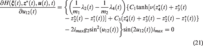
We assume $u_{12}\left(t\right)$ range: $U=[0,\pi )$ regarding the period of both $\sin \left(2u_{12}\left(t\right)\right)$ and ${\sin }^2\left(u_{12}\left(t\right)\right)$ . Equation (21) results in

$$\sin \left(2u_{12}\left(t\right)\right)=0$$

or

$$\begin{array}{l}{\sin }^2(u_{12}(t))=\frac{1}{2i_{max}{g}_2}\left(\frac{1}{m_1}{\xi }_2(t)-\frac{1}{m_2}{\xi }_4(t)\right)\{C_1\tanh \left[\nu (z_4(t)+z_3(t)-z_2(t)-z_1(t))\right]\\ +C_3(z_4(t)+z_3(t)-z_2(t)-z_1(t))\}\end{array}$$

(23)

Let us analyse three disjoint and complementary cases

Case 1: If the right-hand side of (23) is negative, then we have the Hamiltonian maximum (+/– sign change of (21)) at $u_{12}^{\text{*}}\left(t\right)=0$ ; thus $\sin \left(2u_{12}^{\text{*}}\left(t\right)\right)=0$ and ${\sin }^2\left(u_{12}^{\text{*}}\left(t\right)\right)=0$ , i.e. according to (12)

$$i_{12}^{\text{*}}\left({\mathit{u}}^{\text{*}}\left(t\right),t\right)=0$$

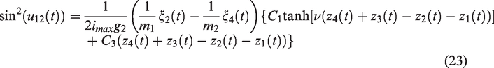
Case 2: If the right-hand side of equation (23) is within the range of [0 1), then we have the Hamiltonian maximum at $u_{12}^{\text{*}}\left(t\right)$  such that

$$\begin{array}{l}{\sin }^2(u_{12}^{\text{*}}(t))=\frac{1}{2i_{max}{g}_2}\left(\frac{1}{m_1}{\xi }_2(t)-\frac{1}{m_2}{\xi }_4(t)\right)\{C_1\tanh \left[\nu (z_4(t)+z_3(t)-z_2(t)-z_1(t))\right]\\ +C_3(z_4(t)+z_3(t)-z_2(t)-z_1(t))\}\end{array}$$

i.e.

$$\begin{array}{l}{i}_{12}^{\text{*}}\left({\mathit{u}}^{\text{*}}\left(t\right),t\right)=\frac{1}{2g_2}\left(\frac{1}{m_1}{\xi }_2\left(t\right)-\frac{1}{m_2}{\xi }_4\left(t\right)\right)\{C_1\tanh \left[\nu \left(z_4\left(t\right)+z_3\left(t\right)-z_2\left(t\right)-z_1\left(t\right)\right)\right]\\ +C_3\left(z_4\left(t\right)+z_3\left(t\right)-z_2\left(t\right)-z_1\left(t\right)\right)\}\end{array}$$

Case 3: If the right-hand side of equation (23) is within the range of [1 ∞), then we have the Hamiltonian maximum at $u_{12}^{\text{*}}\left(t\right)=\pi /2$ , thus

$$i_{12}^{\text{*}}\left({\mathit{u}}^{\text{*}}\left(t\right),t\right)=i_{max}$$

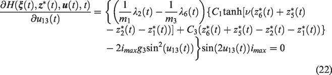
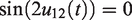
The obtained solution is consistent with. ⁴⁸ The same analysis applied for equation (22) concerning $u_{13}\left(t\right)$ , gives analogical results for $u_{13}^{\text{*}}\left(t\right)$ and $i_{13}^{\text{*}}\left({\mathit{u}}^{\text{*}}\left(t\right),t\right)$ (equation (13)).

Baseline implementation technique

The common approach to the optimal control of nonlinear systems is computation of the optimal control $u^{\text{*}}\left(t\right)$ using the maximum principle by solving the two-point boundary value problem (1)÷(5) offline; however, the so calculated open-loop control suffers from a lack of robustness to operating uncertainties, perturbations of external forces or initial conditions, and to unmodeled dynamics that are always present for highly nonlinear systems. Oates and Smith ¹³ present the examples of complete degradation in control authority when initial conditions or external disturbances are badly assumed or omitted. To improve robustness to various types of uncertainties, the perturbation control technique, among others, is used.^13,37,49 In this method, the generated control signal is based on a simplification (e.g. linearisation) of the system, and adjusted online to attenuate perturbations. However, for highly nonlinear systems with implicit relations between state, co-state and control, proper simplification (linearisation) may be an issue.

To cope with the control authority degradation due to the external disturbances, unmodelled dynamics or conditions change, the approach proposed here (further indicated with one-step optimal or, for simplicity, Optimal control) is to solve the boundary value problem (1)÷(5) at every sample step with the state and co-state dynamics online implementation. Due to the high computational load required online, an optimisation horizon $\left[t_0,t_1\right]$ is assumed: $t_0=0$ , $t_1$ equal to one integration step, aiming for piecewise (one-step) optimality. The MATLAB/Simulink 2016b environment is used. A dedicated level-2 s-function is called at every sample step, using actual external conditions signal(s) value(s), actual state values as initial conditions for equation (1), and terminal condition (5) for co-state. Utilising the bvp4c MATLAB function at every sample step, the boundary value problem is solved, the initial values for the co-state are calculated, and all co-state integrators are reset to these values. bvp4c is a finite difference iterative approach that implements the three-stage Lobatto IIIa formula.^50,51 Alternative iterative approaches are the Adomian decomposition method (ADM), the variational iteration method (VIM), ⁵² the homotopy analysis method (HAM), ⁵³ the homotopy method coupling with the perturbation technique – the homotopy perturbation method (HPM), ⁵⁴ etc., throughout which VIM and HPM are the methods of choice as they can effectively and accurately solve a large class of nonlinear problems including those with strong nonlinearity. They produce rapidly convergent successive approximations, do not require linearisation, do not impose the limitations or assumptions required in classical perturbation methods, while they can overcome the difficulties arising in handling Adomian polynomials or HAM free parameter determination.^55–61

The test conditions parameters are as follows. The primary system (structure) is excited by a harmonic force of amplitude $A\left(P\left(t\right)\right)=61$ N and angular frequency $\omega \left(t\right)\in \left[13.2,31.4\right]$ rd/s (i.e. $\left[2.1,5.0\right]$ Hz). Fixed sample step $t_s={10}^{-3}$  s is adopted ( $t_s=5\cdot {10}^{-4}$  s within the $\left[17.0,18.2\right]$ rd/s i.e. $\left[2.7,2.9\right]$  Hz range for the two-TVA system). An automatic solver is selected, resulting in the ode3 procedure (ode8 is selected within the $\left[17.0,18.2\right]$ rd/s range for the two-TVA system). The weighting factors for the Hamiltonian are assumed so as to minimise the primary system (structure) displacement $x_1$ amplitude: $g_{11}={10}^{21}$ , $g_{12}={10}^6$ ( $g_{11}={10}^{18}$ , $g_{12}=0$ for single TVA), $g_2=g_3=4$ . MR damper continuous control current limitation $i_{max}=0.5$ A is assumed with respect to Lord Rheonetic. ²¹

Alternative techniques

The main problem of online implementation of the maximum principle for the uncertain systems is the fulfilment of the transversality condition (5), requiring high computational load boundary value problem integration. This section addresses that problem and proposes alternative, optimal-based approaches.

Alternative concepts

It may be observed that for most oscillatory systems, the co-state variable $\xi \left(t\right)$ changes sign every particular period of time (e.g. half of the oscillation period i.e. $t_1=\pi /\omega$ ) as the co-state is periodic for problems with periodic state conditions. If the co-state is a scalar, one may simply assume the final time $t_1^N$ at the current Nth step optimal problem task to be a moment of the co-state being equal to zero ( $\xi \left(t_1^N\right)=0$ ), and immediately start new, the N + 1th step optimal problem task with $t_0^{N+1}=t_1^N$ . If the co-state is a vector, the final time $t_1^N$ at the current Nth step optimal problem task may be assumed as a moment of the co-state dominant element ( ${\xi }_1^{}$ in the current problem) being equal to zero ( ${\xi }_1^{}\left(t_1^N\right)=0,\text{ while }{\hspace{0.17em}}_{\xi }^{2÷6}\left(t_1^N\right)\ne 0$ ), and investigated the error of this approach. Analogically, the N + 1th step optimal problem task start time will be set: $t_0^{N+1}=t_1^N$ by resetting to zero all the co-state integrators at $t_r=t_0^{N+1}$ ( $t_r$ – reset time). If the calculated terminal condition (5) error is negligible, this may save the large computational load. This approach is further indicated with the Q-O Ksi1 (Quasi-Optimal, ${\xi }_1^{}$  sign change based resetting approach). Along with the Q-O Ksi1 solution, a similar approach based on the resetting of all the co-state integrators to zero every $z_1$  sign change, with the terminal condition (5) error calculation, was tested. This approach is further indicated with the Q-O Z1 (Quasi-Optimal, $z_1$  sign change based resetting approach).

Another concept to avert a large computational load boundary value problem integration is the utilisation of the very short time range $\left[t_0,t_1\right]$ basis optimal problem task instead of the exemplary half oscillation period or one integration step time range basis ( $t_1\ll \pi /\omega$ and $t_s={10}^{-5}$  s were assumed) using the high frequency resetting function and zero initial conditions for all the co-state integrators to enhance the influence of the ‘ $-g\left(\mathit{z}\left(t\right),\mathit{u}\left(t\right),t\right)$ ' term in (3) and so diminish the $\mathit{\xi }\left(t_1\right)$ value and thus the influence of the equality (5) error. Again, if the calculated error is negligible, this may save a large computational load at the expense of a higher sampling rate. Piecewise quasi-optimality is assumed to be fulfilled. This approach is further indicated with the Q-O HF (Quasi-Optimal, High Frequency resetting approach).

Calculus of the errors

The calculus of the errors of the alternative, quasi-optimal approaches is based on the elementary proof of the maximum principle for the problem with the free right end point. ⁴⁷ Some basic steps of this proof are cited here.

Let $\tau$ be a continuity point of the optimal control ${\mathit{u}}^{\text{*}}\left(t\right)$ , and the needle-like variation of ${\mathit{u}}^{\text{*}}\left(t\right)$ is defined as

$${\mathit{u}}^{\lambda }\left(t\right)=\{\begin{array}{c}{\mathit{u}}^{\text{*}}\left(t\right), \mathrm{if} t\notin [\tau -\lambda ,\tau ) \\ v, \mathrm{if} t\in [\tau -\lambda ,\tau )\end{array}$$

(24)where $\mathit{v}\in U$ is fixed. We denote by ${\mathit{z}}^{\lambda }\left(t\right)$ the solution of (1) which corresponds to the control ${\mathit{u}}^{\lambda }\left(t\right)$ . For $t\in [t_0,\tau -\lambda ]$ we have ${\mathit{z}}^{\lambda }\left(t\right)={\mathit{z}}^{\text{*}}\left(t\right)$ . For sufficiently small $\lambda$ , the vector valued function ${\mathit{z}}^{\lambda }\left(t\right)$ is defined on $[\tau -\lambda ,\tau ]$ . The states ${\mathit{z}}^{\lambda }\left(\tau \right)$ and ${\mathit{z}}^{\text{*}}\left(\tau \right)$ are arbitrary close to each other as control functions ${\mathit{u}}^{\lambda }\left(t\right)$ and ${\mathit{u}}^{\text{*}}\left(t\right)$ are arbitrary close in $[t_0,\tau ]$ . Thus ${\mathit{z}}^{\lambda }\left(t\right)$ is a small perturbation of ${\mathit{z}}^{\text{*}}\left(\tau \right)$ in $\left[\tau ,t_1\right].$

If the control ${\mathit{u}}^{\text{*}}\left(t\right)$ is continuous at the point $\tau$ , then

$$\begin{array}{l}{\mathit{z}}^{\text{*}}\left(\tau \right)={\mathit{z}}^{\text{*}}\left(\tau -\lambda \right)+\lambda {\dot{z}}^{\text{*}}\left(\tau -\lambda \right)+\mathit{o}\left(\lambda \right)={\mathit{z}}^{\text{*}}\left(\tau -\lambda \right)+\lambda \mathit{f}\left({\mathit{z}}^{\text{*}}\left(\tau -\lambda \right),{\mathit{u}}^{\text{*}}\left(\tau -\lambda \right),\tau -\lambda \right)+\mathit{o}\left(\lambda \right)\\ {\mathit{z}}^{\lambda }\left(\tau \right)={\mathit{z}}^{\text{*}}\left(\tau -\lambda \right)+\lambda \mathit{f}\left({\mathit{z}}^{\text{*}}\left(\tau -\lambda \right),\mathit{v},\tau -\lambda \right)+\mathit{o}\left(\lambda \right)\end{array}$$

There exists a limit

$$\mathit{y}\left(\tau \right)=\underset{\lambda \to 0}{\lim }\frac{{\mathit{z}}^{\lambda }\left(\tau \right)-{\mathit{z}}^{\text{*}}\left(\tau \right)}{\lambda }=\mathit{f}\left({\mathit{z}}^{\text{*}}\left(\tau \right),\mathit{v},\tau \right)-\mathit{f}\left({\mathit{z}}^{\text{*}}\left(\tau \right),{\mathit{u}}^{\text{*}}\left(\tau \right),\tau \right)$$

(25)

For $\lambda >0$  sufficiently small, the vector valued functions ${\mathit{z}}^{\lambda }\left(t\right)$ are defined also on $[\tau ,t_1]$ and converge uniformly to ${\mathit{z}}^{\text{*}}\left(t\right)$ . For any $t\in [\tau ,t_1]$ there exists a limit

$$\mathit{y}\left(t\right)=\underset{\lambda \to 0}{\lim }\frac{{\mathit{z}}^{\lambda }\left(t\right)-{\mathit{z}}^{\text{*}}\left(t\right)}{\lambda }=\mathit{y}\left(\tau \right)+{\displaystyle {\int }_{\tau }^t{\mathit{f}}_z\left({\mathit{z}}^{\text{*}}\left(\theta \right),{\mathit{u}}^{\text{*}}\left(\theta \right),\theta \right)\mathit{y}\left(\theta \right)\text{d}\theta }$$

(26)

Thus, on $[\tau ,t_1]$ the function $\mathit{y}\left(t\right)$ is the solution of

$$\dot{y}\left(t\right)={\mathit{f}}_z\left({\mathit{z}}^{\text{*}}\left(t\right),{\mathit{u}}^{\text{*}}\left(t\right),t\right)\mathit{y}\left(t\right)$$

(27)

with the initial condition (25), thus

$$\frac{d}{dt}\left({\mathit{\xi }}^T\left(t\right)\mathit{y}\left(t\right)\right)=g_z\left({\mathit{z}}^{\text{*}}\left(t\right),{\mathit{u}}^{\text{*}}\left(t\right),t\right)\mathit{y}\left(t\right)$$

and so

$${\mathit{\xi }}^T\left(t\right)\mathit{y}\left(t\right)=-{\displaystyle {\int }_t^{t_1}{g}_z\left({\mathit{z}}^{\text{*}}\left(\theta \right),{\mathit{u}}^{\text{*}}\left(\theta \right),\theta \right)\mathit{y}\left(\theta \right)\text{d}\theta +{\mathit{\xi }}^T\left(t_1\right)\mathit{y}\left(t_1\right)}$$

(28)

Here, in the elementary proof of the maximum principle, it is assumed: ${\mathit{\xi }}^{\text{*}}\left(t_1\right)=0$ according to equation (5); however, in our implementation we have either: ${\xi }_1^{}\left(t_1\right)=0$ and ${\hspace{0.17em}}_{\xi }^{2÷6}\left(t_1\right)\ne 0$ , or: ${\hspace{0.17em}}_{\xi }^{1÷6}\left(t_1\right)\ne 0$ , thus we proceed for $t=\tau$ according to equation (25)

$$\begin{array}{l}{\mathit{\xi }}^T\left(\tau \right)\left[\mathit{f}\left({\mathit{z}}^{\text{*}}\left(\tau \right),{\mathit{u}}^{\text{*}}\left(\tau \right),\tau \right)-f\left({\mathit{z}}^{\text{*}}\left(\tau \right),\mathit{v},\tau \right)\right]={\displaystyle {\int }_{\tau }^{t_1}{g}_z\left({\mathit{z}}^{\text{*}}\left(\theta \right),{\mathit{u}}^{\text{*}}\left(\theta \right),\theta \right)\mathit{y}\left(\theta \right)\text{d}\theta }-{\mathit{\xi }}^T\left(t_1\right)\mathit{y}\left(t_1\right)\end{array}$$

(29)

For $\left({\mathit{z}}^{\text{*}}\left(t\right),{\mathit{u}}^{\text{*}}\left(t\right)\right)$ being an optimal control process

$$\underset{\lambda \to 0}{\lim }\frac{G\left({\mathit{z}}^{\lambda }\left(t\right),{\mathit{u}}^{\lambda }\left(t\right)\right)-G\left({\mathit{z}}^{\text{*}}\left(t\right),{\mathit{u}}^{\text{*}}\left(t\right)\right)}{\lambda }\ge 0$$

(30)thus

$$\begin{array}{l}\underset{\lambda \to 0}{\lim }\frac{1}{\lambda }{\displaystyle {\int }_{\tau -\lambda }^{\tau }g\left({\mathit{z}}^{\lambda }\left(\theta \right),\mathit{v},\theta \right)-g\left({\mathit{z}}^{\text{*}}\left(\theta \right),{\mathit{u}}^{\text{*}}\left(\theta \right),\theta \right)\text{d}\theta }+\underset{\lambda \to 0}{\lim }\frac{1}{\lambda }{\displaystyle {\int }_{\tau }^{t_1}g\left({\mathit{z}}^{\lambda }\left(\theta \right),{\mathit{u}}^{\lambda }\left(\theta \right),\theta \right)-g\left({\mathit{z}}^{\text{*}}\left(\theta \right),{\mathit{u}}^{\text{*}}\left(\theta \right),\theta \right)\text{d}\theta \ge 0}\\ g\left({\mathit{z}}^{\text{*}}\left(\tau \right),\mathit{v},\tau \right)-g\left({\mathit{z}}^{\text{*}}\left(\tau \right),{\mathit{u}}^{\text{*}}\left(\tau \right),\tau \right)\ge -{\displaystyle {\int }_{\tau }^{t_1}{g}_z\left({\mathit{z}}^{\text{*}}\left(\theta \right),{\mathit{u}}^{\text{*}}\left(\theta \right),\theta \right)\mathit{y}\left(\theta \right)\text{d}\theta }\end{array}$$

(31)

Using equation (29), we obtain

$$\begin{array}{l}g\left({\mathit{z}}^{\text{*}}\left(\tau \right),\mathit{v},\tau \right)-g\left({\mathit{z}}^{\text{*}}\left(\tau \right),{\mathit{u}}^{\text{*}}\left(\tau \right),\tau \right)\ge {\mathit{\xi }}^T\left(\tau \right)\left[\mathit{f}\left({\mathit{z}}^{\text{*}}\left(\tau \right),\mathit{v},\tau \right)-\mathit{f}\left({\mathit{z}}^{\text{*}}\left(\tau \right),{\mathit{u}}^{\text{*}}\left(\tau \right),\tau \right)\right]-{\mathit{\xi }}^T\left(t_1\right)\mathit{y}\left(t_1\right)\end{array}$$

(32)Hence

$$\begin{array}{l}-g\left({\mathit{z}}^{\text{*}}\left(\tau \right),{\mathit{u}}^{\text{*}}\left(\tau \right),\tau \right)+{\mathit{\xi }}^T\left(\tau \right)\mathit{f}\left({\mathit{z}}^{\text{*}}\left(\tau \right),{\mathit{u}}^{\text{*}}\left(\tau \right),\tau \right)\ge -g\left({\mathit{z}}^{\text{*}}\left(\tau \right),\mathit{v},\tau \right)+{\mathit{\xi }}^T\left(\tau \right)\mathit{f}\left({\mathit{z}}^{\text{*}}\left(\tau \right),\mathit{v},\tau \right)-{\mathit{\xi }}^T\left(t_1\right)y\left(t_1\right)\end{array}$$

This can be written in the equivalent form

$$H\left(\mathit{\xi }\left(\tau \right),{\mathit{z}}^{\text{*}}\left(\tau \right),{\mathit{u}}^{\text{*}}\left(\tau \right),\tau \right)\ge H\left(\mathit{\xi }\left(\tau \right),{\mathit{z}}^{\text{*}}\left(\tau \right),\mathit{v},\tau \right)-{\mathit{\xi }}^T\left(t_1\right)\mathit{y}\left(t_1\right)$$

(33)where $\tau$ is an arbitrary continuity point of the control ${\mathit{u}}^{\text{*}}\left(\tau \right)$ , while $\mathit{v}$ is an arbitrary element of the set $U$ . Thus, for $\mathbf{\xi }\left(t_1\right)=\mathbf{0},$ equation (6) holds for all the continuity points of the control ${\mathit{u}}^{\text{*}}\left(\tau \right)$ .

To investigate the regarded approach error resulting from taking the assumption either: ${\xi }_1^{}\left(t_1\right)=0$ and ${\hspace{0.17em}}_{\xi }^{2÷6}\left(t_1\right)\ne 0$ , or: ${\hspace{0.17em}}_{\xi }^{1÷6}\left(t_1\right)\ne 0$ , instead of ${\hspace{0.17em}}_{\xi }^{1÷6}\left(t_1\right)=0$ (5), the product ${\mathit{\xi }}^T\left(t_1\right)\mathit{y}\left(t_1\right)$ in equation (33) is estimated for different values of $\tau$ , calculating $\mathit{y}\left(t_1\right)$ with the use of equation (27). The initial condition $\mathit{y}\left(\tau \right)$ based on the formula (25) is assumed: $\mathit{y}\left(\tau \right)=-\mathit{f}\left({\mathit{z}}^{\text{*}}\left(\tau \right),{\mathit{u}}^{\text{*}}\left(\tau \right),\tau \right)$ , which is assessed to be of the order of magnitude equal or higher than $\mathit{f}\left({\mathit{z}}^{\text{*}}\left(\tau \right),\mathit{v},\tau \right)-\mathit{f}\left({\mathit{z}}^{\text{*}}\left(\tau \right),{\mathit{u}}^{\text{*}}\left(\tau \right),\tau \right)$ (being the right-hand side of equation (25)), regarding the values of the terms present in the right-hand side of equation (9) for the assumed system parameters (see Table 1), $P\left(t\right)$ , $\omega \left(t\right)$ ranges, and the MR damper resistance forces (10)(10’)(11) ranges limited by $i_{12}\left(\mathit{u}\left(t\right),t\right)$ (12), $i_{13}\left(\mathit{u}\left(t\right),t\right)$ (13) constraints, that are in turn limited by the $\mathit{u}\left(t\right)\in U$ requirement (  $\mathit{f}\left({\mathit{z}}^{\text{*}}\left(\tau \right),\mathit{v},\tau \right)$ is of the order of $\mathit{f}\left({\mathit{z}}^{\text{*}}\left(\tau \right),{\mathit{u}}^{\text{*}}\left(\tau \right),\tau \right)$ as $\mathit{v}\in U$ in equation (24)).

Based on equation (33), for $H\left(\mathit{\xi }\left(\tau \right),{\mathit{z}}^{\text{*}}\left(\tau \right),{\mathit{u}}^{\text{*}}\left(\tau \right),\tau \right)\ne 0$ , we obtain

$$\frac{H\left(\mathit{\xi }\left(\tau \right),{\mathit{z}}^{\text{*}}\left(\tau \right),\mathit{v},\tau \right)}{H\left(\mathit{\xi }\left(\tau \right),{\mathit{z}}^{\text{*}}\left(\tau \right),{\mathit{u}}^{\text{*}}\left(\tau \right),\tau \right)}\le 1+\epsilon \left(\tau \right)$$

(34)where the error $\epsilon \left(\tau \right)$ is

$$\epsilon \left(\tau \right)=\frac{{\mathit{\xi }}^T\left(t_1\right)\mathit{y}\left(t_1\right)}{H\left(\mathit{\xi }\left(\tau \right),{\mathit{z}}^{\text{*}}\left(\tau \right),{\mathit{u}}^{\text{*}}\left(\tau \right),\tau \right)}$$

(35)

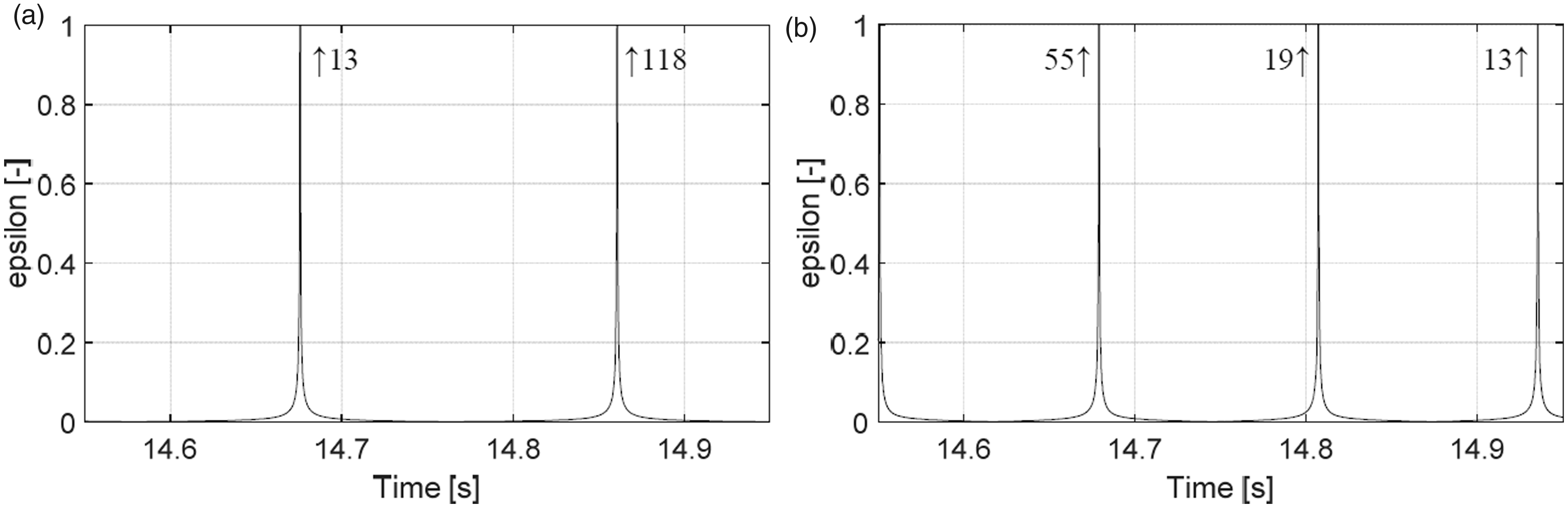
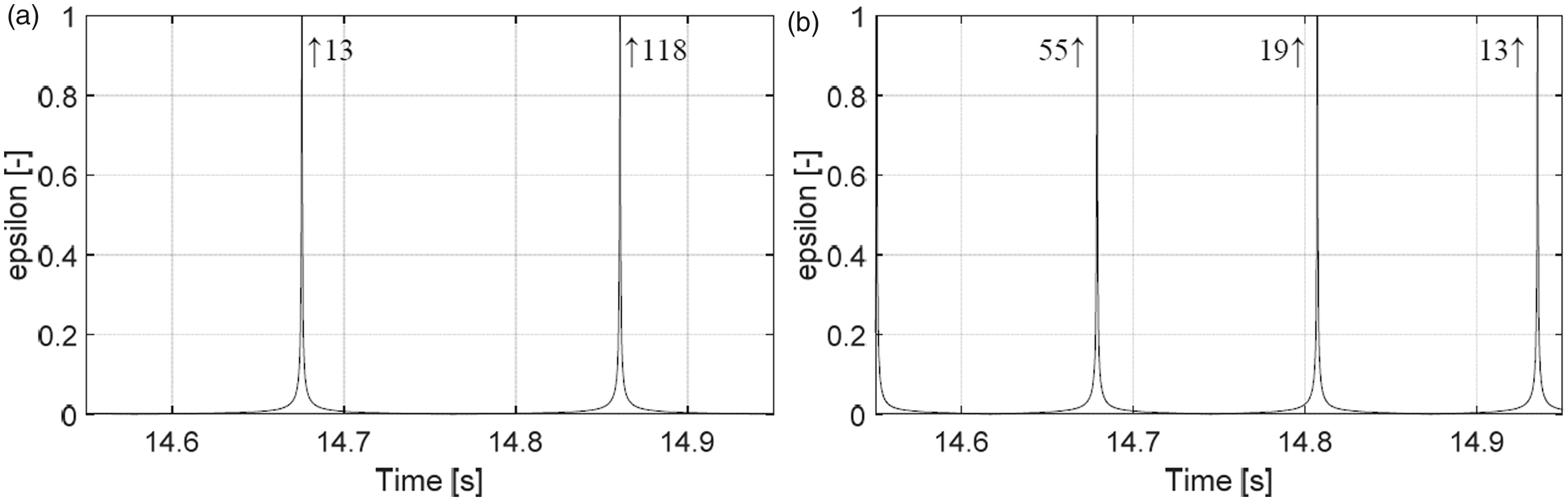
For the Q-O Ksi1 and Q-O Z1 approaches, the values of $\tau$ from the range of $[t_0,t_1)$ with ${10}^{-3}$  s ( ${10}^{-5}$  s for the Q-O HF concept) step were adopted and: $t_0=0$ , $t_1=\pi /\omega$ ( $t_1={10}^{-4}$  s for the Q-O HF concept), assuming ${\xi }_1^{}$ (or $z_1$ , respectively) sign change every half of the oscillation period. Using equation (35), for each assumed value of $\tau$ , a quotient $\epsilon \left(\tau \right)$ (regarded approach error) was assessed according to the above concept. As a result, non-negligible (over $1$ in wide time ranges) $\epsilon \left(\tau \right)$ values were obtained for both the Q-O Ksi1 and Q-O Z1 approach. Thus these two solutions are further ignored. The Q-O HF approach copes better with the problem of $\epsilon \left(\tau \right)$ error – the values of a quotient $\epsilon \left(\tau \right)$ for most of the time samples are assessed to be negligible, thus control results may be considered credible in wide time ranges. The exemplary $\epsilon \left(\tau \right)$ patterns for the 2.7 Hz (point A in the primary system/structure displacement amplitude output frequency responses, Figure 4) and 3.9 Hz (point C in Figure 4) excitation frequencies are presented in Figures 2 ( $\tau =0$  s) and 3 ( $\tau ={10}^{-5}$  s). For higher $\tau$ values, no significant change in the assessed $\epsilon \left(\tau \right)$ patterns is observed. For simplicity, the results of the Q-O HF approach are further indicated as the Quasi-Optimal control.

Figure 2.

Assessed ε(τ) patterns for τ = 0 s at: 2.7 Hz (a), 3.9 Hz (b).

Modified ground-hook law

On the basis of the Hamiltonian principle-based MR damper current determination equations (21) to (23), the modified ground hook control is derived. It was originally introduced^5,6 aiming at primary system/structure amplitude minimisation as a design criteria. Let us concentrate on formula (23). The sign of: $\left\{C_1\tanh \left[\nu \left(z_4\left(t\right)+z_3\left(t\right)-z_2\left(t\right)-z_1\left(t\right)\right)\right]+C_3\left(z_4\left(t\right)+z_3\left(t\right)-z_2\left(t\right)-z_1\left(t\right)\right)\right\}$ is always the same as the sign of: $F_{12}\left(\mathit{z}\left(t\right),\mathit{u}\left(t\right),t\right)$ , as $i_{12}\left(\mathit{u}\left(t\right),t\right)\ge 0$ always holds and all parameters $C_1$ , $C_2$ , $C_3$ , $C_4$ , $\nu$ , $p$ present in the MR damper forward model (10) ⁴⁶ are positive. Let us now regard the sign of $\left(\frac{1}{m_1}{\xi }_2\left(t\right)-\frac{1}{m_2}{\xi }_4\left(t\right)\right)$ . As $2g_{11}{z}_1^{}\left(t\right)$ is the dominant term of the first-row in matrix equation (4) right-hand side, ${\xi }_2\left(t\right)$ and $2g_{12}{z}_2^{}\left(t\right)$ are the dominant terms of the second-row in equation (4) right-hand side, while $g_{11}$ is assumed to be at least the 15th order of the magnitude greater than $g_{12}$ (considering the design criteria) with $A(z_2\left(t\right))=\omega \left(t\right)A(z_1\left(t\right))$ ( $A(•)$  states for the amplitude), the formula

$$A({\xi }_2\left(t\right))\hspace{0.17em}\approx \hspace{0.17em}A({\xi }_1\left(t\right))/\omega \left(t\right)$$

(36)

gives sufficiently precise approximation of ${\xi }_1\left(t\right)$ and ${\xi }_2\left(t\right)$ amplitudes relation, with the ${\xi }_2\left(t\right)$ phase delayed with regard to the ${\xi }_1\left(t\right)$ phase by: $\text{arg}({\xi }_1\left(t\right))-\text{arg}({\xi }_2\left(t\right))\hspace{0.17em}\approx \hspace{0.17em}\pi /2$ , assuming an oscillation pattern characterised by single dominant angular frequency $\omega \left(t\right)$ . Further, by analysing the third-row (implicating ${\xi }_3\left(t\right)$ ) and the fourth-row (implicating ${\xi }_4\left(t\right)$ ) equation of (4) in relation to ${\xi }_2\left(t\right)$ , as well as the values of $k_2/m_1$ , $k_2/m_2$ , ${\tilde{F}}_{12}\left({\mathit{z}}^{\text{*}}\left(t\right),{\mathit{u}}^{\text{*}}\left(t\right),t\right)/m_1$ , ${\tilde{F}}_{12}\left({\mathit{z}}^{\text{*}}\left(t\right),{\mathit{u}}^{\text{*}}\left(t\right),t\right)/m_2$ for the assumed $P\left(t\right)$ and $\omega \left(t\right)$ ranges, it is concluded that inequality: $A\left({\xi }_2\left(t\right)/m_1\right)>A\left({\xi }_4\left(t\right)/m_2\right)$ holds with negligible phase shift: $\text{arg}\left({\xi }_2\left(t\right)\right)-\text{arg}\left({\xi }_4\left(t\right)\right)\approx 0$ , and

$$sgn\left(\frac{1}{m_1}{\xi }_2\left(t\right)-\frac{1}{m_2}{\xi }_4\left(t\right)\right)\approx sgn\left({\xi }_2\left(t\right)\right)$$

(37)

From the above considerations on the system (4) first-row and second-row right-hand sides

$$sgn\left({\xi }_2\left(t\right)\right)\approx sgn\left(-z_1\left(t\right)\right)$$

(38)thus

$$sgn\left(\frac{1}{m_1}{\xi }_2\left(t\right)-\frac{1}{m_2}{\xi }_4\left(t\right)\right)\approx sgn\left(-z_1\left(t\right)\right)$$

(39)

The simulations prove that formula (39) gives an adequately precise approximation of the $\left(\frac{1}{m_1}{\xi }_2\left(t\right)-\frac{1}{m_2}{\xi }_4\left(t\right)\right)$ sign, assuming that equation (5) holds or $\epsilon \left(\tau \right)$ is negligible for most of the time samples – more details on this in Remark further on this section. As both $g_2$ and $i_{max}$ are positive, the equation (23) discussion (Case 1, 2, 3) implicates that $i_{12}\left(\mathit{u}\left(t\right),t\right)$ is nonzero if and only if the signs of $\left(\frac{1}{m_1}{\xi }_2\left(t\right)-\frac{1}{m_2}{\xi }_4\left(t\right)\right)$ and $\left\{C_1\tanh \left[\nu \left(z_4\left(t\right)+z_3\left(t\right)-z_2\left(t\right)-z_1\left(t\right)\right)\right]+C_3\left(z_4\left(t\right)+z_3\left(t\right)-z_2\left(t\right)-z_1\left(t\right)\right)\right\}$ are equal, while $i_{12}\left(\mathit{u}\left(t\right),t\right)$ is zero in the opposite case. This leads to the formula

$$\begin{array}{l}{i}_{12}\left(\mathit{u}\left(t\right),t\right)\\ =\{\begin{array}{rr}\hfill \frac{1}{2g_2}\left(\frac{1}{m_1}{\xi }_2\left(t\right)-\frac{1}{m_2}{\xi }_4\left(t\right)\right)\left\{\begin{array}{c}{C}_1\tanh \left[\nu \left(z_4\left(t\right)+z_3\left(t\right)-z_2\left(t\right)-z_1\left(t\right)\right)\right]\\ +C_3\left(z_4\left(t\right)+z_3\left(t\right)-z_2\left(t\right)-z_1\left(t\right)\right)\end{array}\right\},& \hfill \mathrm{if}{F}_{12}\left(\mathit{z}\left(t\right),\mathit{u}\left(t\right),t\right)z_1\left(t\right)<0\\ \hfill 0,& \hfill \mathrm{if}{F}_{12}\left(\mathit{z}\left(t\right),\mathit{u}\left(t\right),t\right)z_1\left(t\right)\ge 0\end{array}\end{array}$$

(40)

giving a semi-continuous optimal-based control current pattern (being the modified continuous displacement ground-hook law). The boundary value problem solving is necessary for the $i_{12}\left(\mathit{u}\left(t\right),t\right)$ value calculation, only if: $F_{12}\left(\mathit{z}\left(t\right),\mathit{u}\left(t\right),t\right)z_1\left(t\right)<0$ holds. However, the (one-step) Optimal control baseline approach implementation for adequately high $g_{11}$ value (primary system/structure displacement $x_1$ amplitude minimisation priority) generates a two level control pattern with two values: $i_{ma\text{x}}$ when: $F_{12}\left(\mathit{z}\left(t\right),\mathit{u}\left(t\right),t\right)z_1\left(t\right)<0$ holds, and 0 in the opposite case (see Figure 6, note that: $z_1=x_1$ ). Thus the formula

$$i_{12}\left(\mathit{u}\left(t\right),t\right)=\{\begin{array}{cc}{i}_{max},& \mathrm{if}{F}_{12}\left(\mathit{z}\left(t\right),\mathit{u}\left(t\right),t\right)z_1\left(t\right)<0\\ 0,& \mathrm{if}{F}_{12}\left(\mathit{z}\left(t\right),\mathit{u}\left(t\right),t\right)z_1\left(t\right)\ge 0\end{array}$$

(41)gives a two-level optimal based control current pattern, being the modified two-level displacement ground-hook law stated by the author earlier ^5,6 (note that the opposite sign concept was adopted for the MR damper force modelling this time). In practice, the modified two-level displacement ground-hook law (41) (indicated further as Mod.GND) is the simple implementation of the optimal control for the case when the primary system/structure displacement amplitude minimisation is the sole objective (see Figures 5 and 6 vs. Figure 8). This approach is further collated with the standard displacement ground-hook law (indicated as the Ground-Hook)⁶³

$$i_{12}\left(\mathit{u}\left(t\right),t\right)=\{\begin{array}{cc}{i}_{max},& \mathrm{if}\left(z_4\left(t\right)-z_2\left(t\right)\right)z_1\left(t\right)<0\\ 0,& \mathrm{if}\left(z_4\left(t\right)-z_2\left(t\right)\right)z_1\left(t\right)\ge 0\end{array}$$

(42)

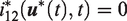
The same analysis with similar results may be applied to formula (22), giving the optimal-based control current pattern $i_{13}\left(\mathit{u}\left(t\right),t\right)$ , being the modified two-level displacement ground-hook law for the damper MRD₁₃.

Remark:

The boundary value problem solving thus appropriate co-state initial values setting leads to the fulfilment of the terminal condition (5) as for the Optimal control baseline approach. This in turn leads to ${\xi }_2\left(t\right)$ and ${\xi }_4\left(t\right)$ values alteration with respect to the quasi-optimal approaches with zero co-state initial values assumption. However, it may be noted that: $sgn(\frac{1}{m_1}{\xi }_2\left(t\right)-\frac{1}{m_2}{\xi }_4\left(t\right))\approx sgn\left({\xi }_2\left(t\right)\right)\approx sgn\left(-z_1\left(t\right)\right)$ holds for both the baseline Optimal control, and Quasi-Optimal (Q-O HF) control approach for all time samples, but their countable number, excluding the samples when – using the Q-O HF concept – the co-state integrators are reset to zero thus: $\mathit{\xi }\left(t_r\right)=\mathbf{0}$ (this is also consistent with the negligible $\epsilon \left(\tau \right)$ error values assessed for most of the time samples – see Figures 2 and 3), in contrary to, e.g., the Q-O Ksi1 approach, resulting in: $sgn(\frac{1}{m_1}{\xi }_2\left(t\right)-\frac{1}{m_2}{\xi }_4\left(t\right))\approx sgn({\xi }_2(t))$ patterns significantly perturbed in relation to $sgn\left(-z_1\left(t\right)\right)$ patterns (and to Optimal control respective sign patterns) by the detrimental co-state resetting conditions (leading concurrently to high $\epsilon \left(\tau \right)$ error values in wide time ranges, as stated in the Calculus of the errors section).

Figure 3.

Assessed $\epsilon \left(\tau \right)$ patterns for $\tau ={10}^{-5}$ s at: 2.7 Hz (a), 3.9 Hz (b).

Vibration control results

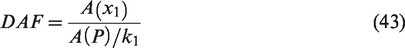
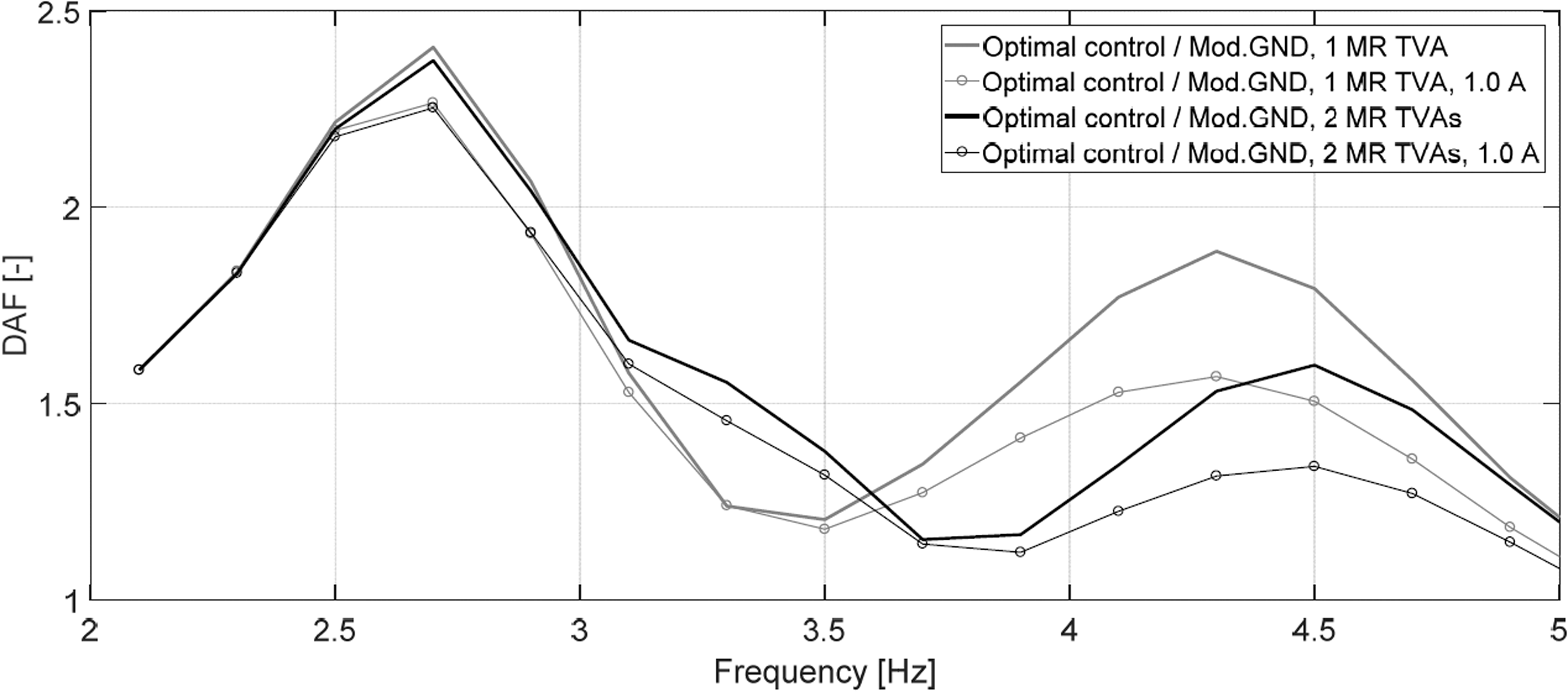
The efficiency of the proposed solutions is analysed based on Dynamic Amplification Factor (DAF) frequency characteristics along with $x_1$ , $x_2$ , $x_3$ , $i_{12}$ , $i_{13}$ , and $\overline{F_{12}}$ time patterns (arguments of the variables are hereinafter omitted for clarity of presentation). Figure 4 presents the DAF frequency characteristics for the system with one or two MR TVAs and the implementation of the Optimal control, Quasi-Optimal control, and optimally tuned passive TVA(s) (for details see Section 3), according to equation (43)

$$DAF=\frac{A\left(x_1\right)}{A\left(P\right)/k_1}$$

(43)

Figure 4.

Dynamic Amplification Factor (DAF) frequency characteristics: Passive damper vs. Optimal control vs. Quasi-Optimal control.

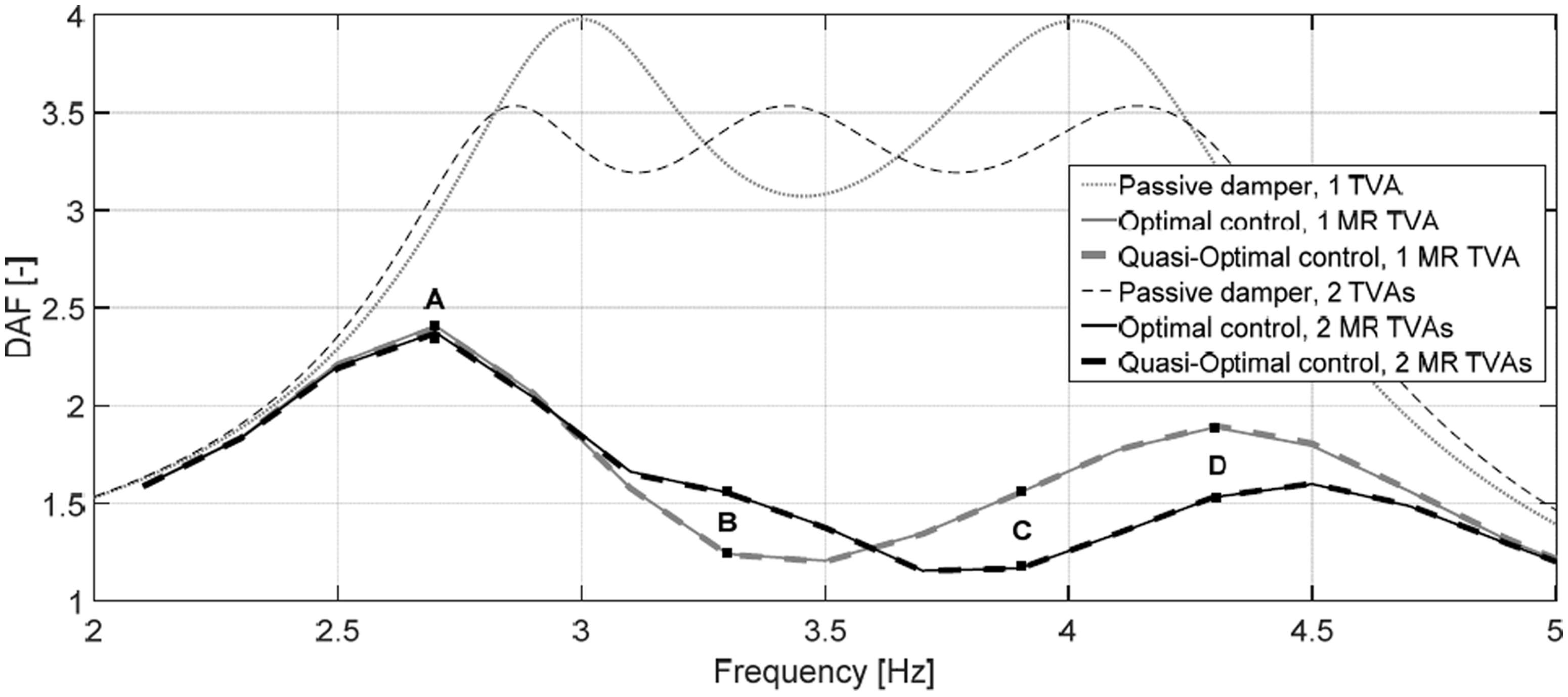
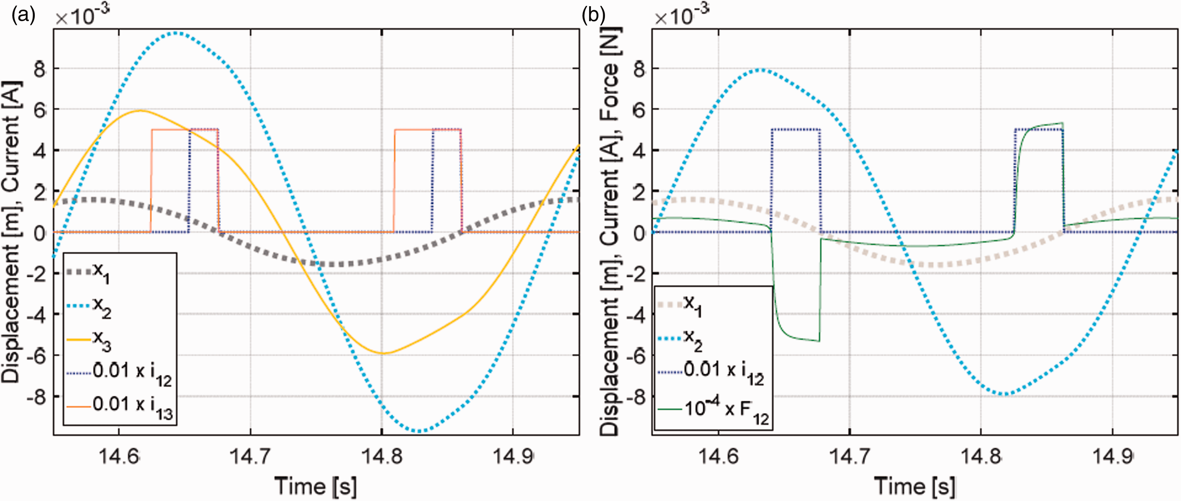
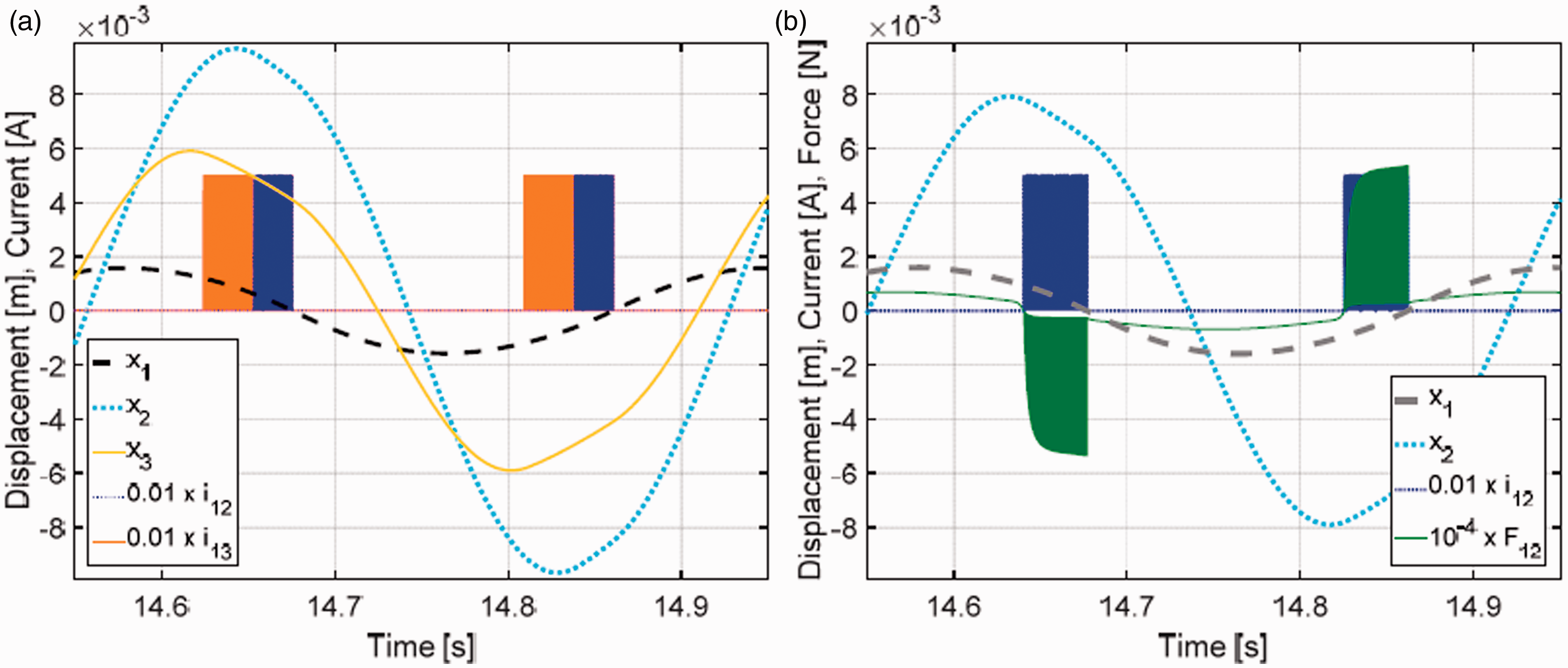
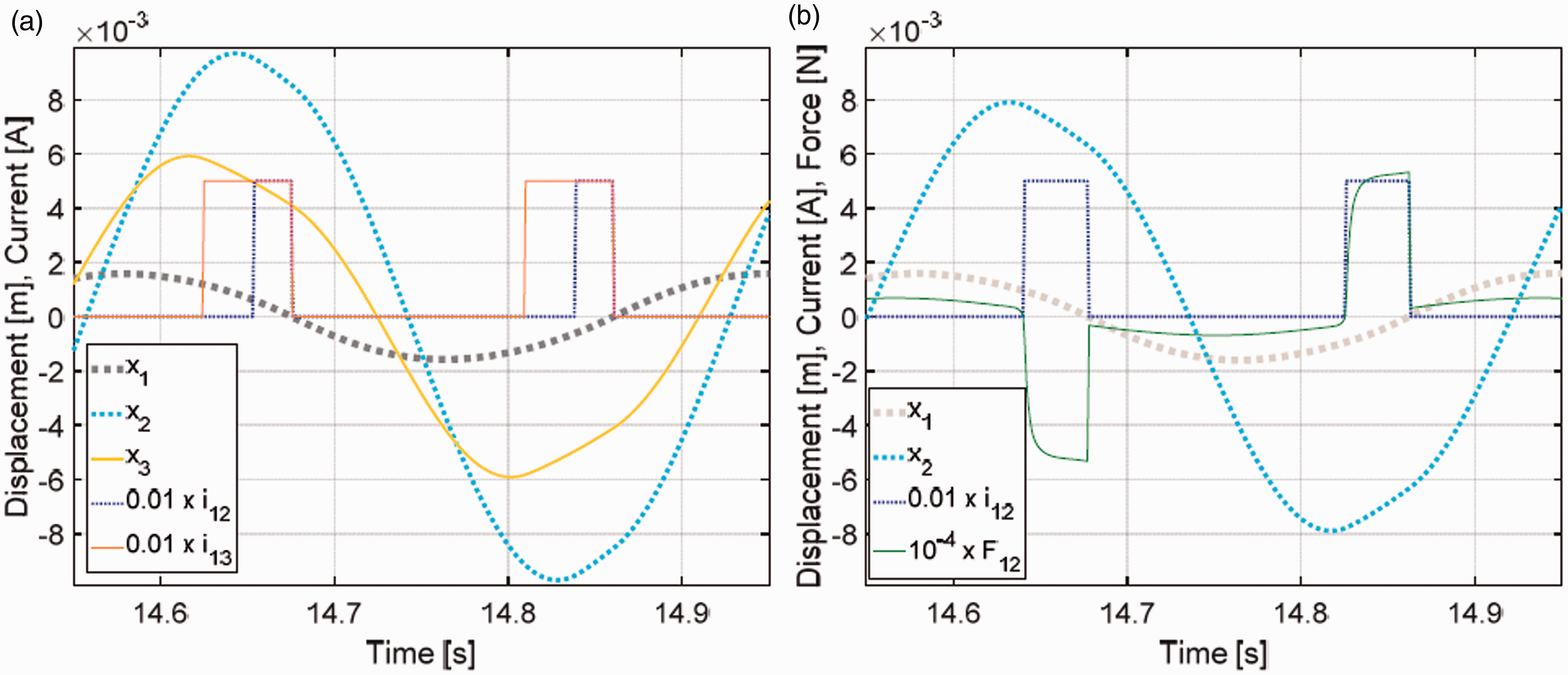
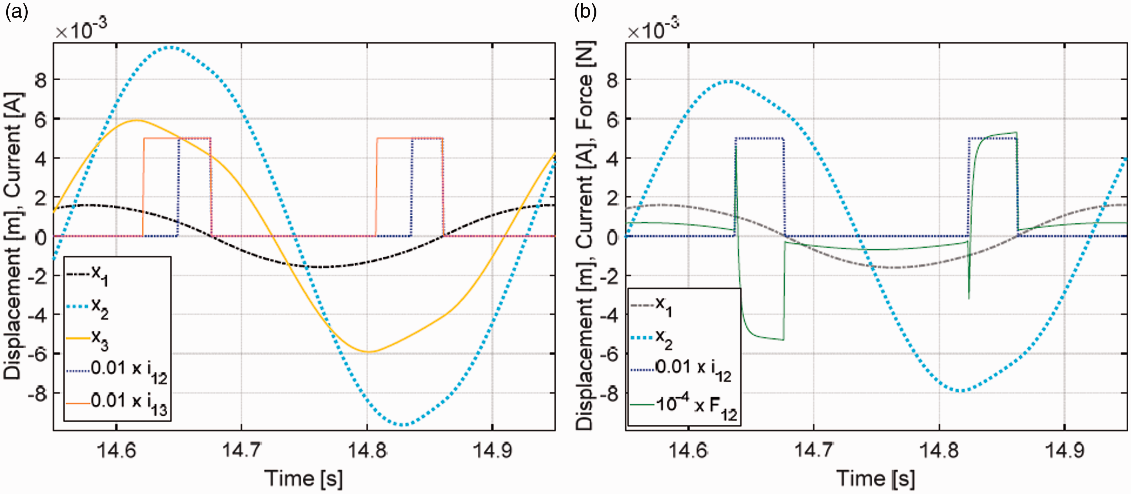
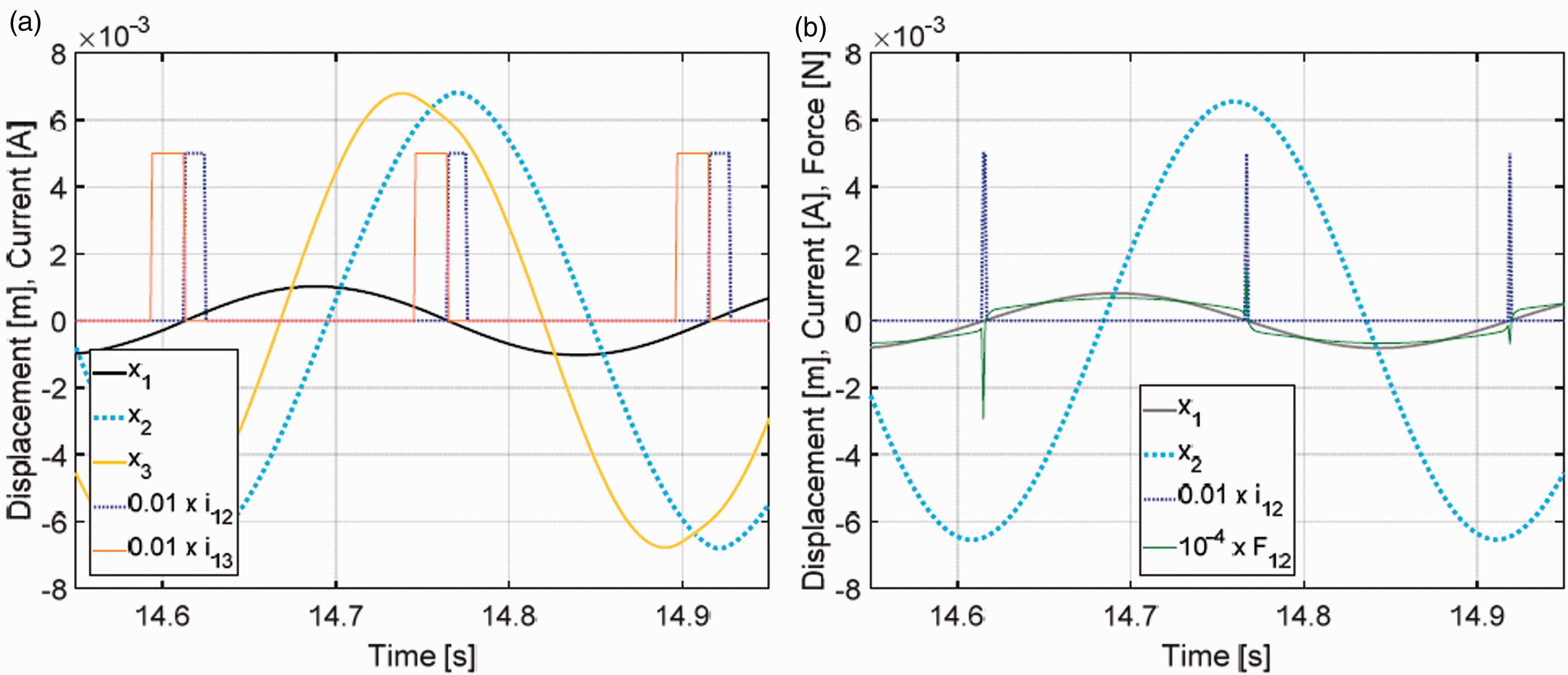
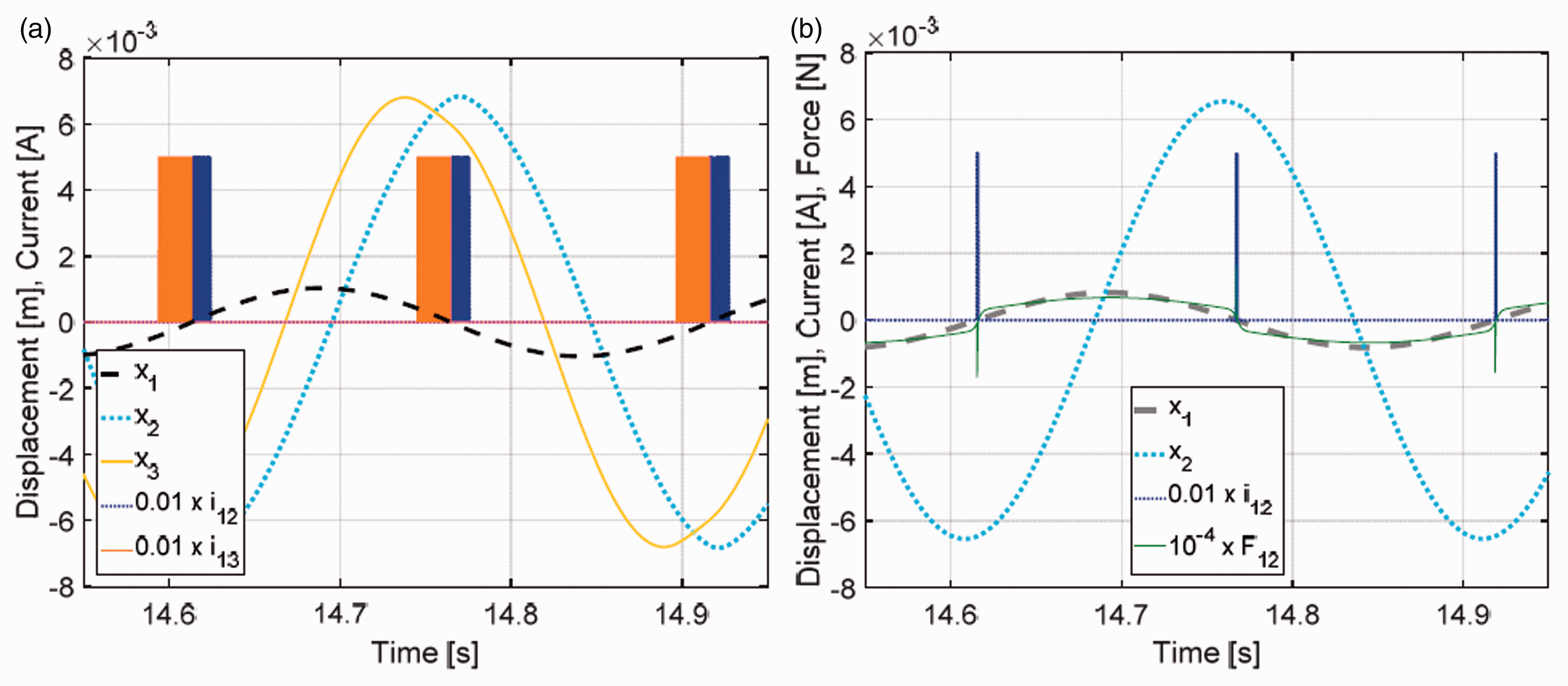
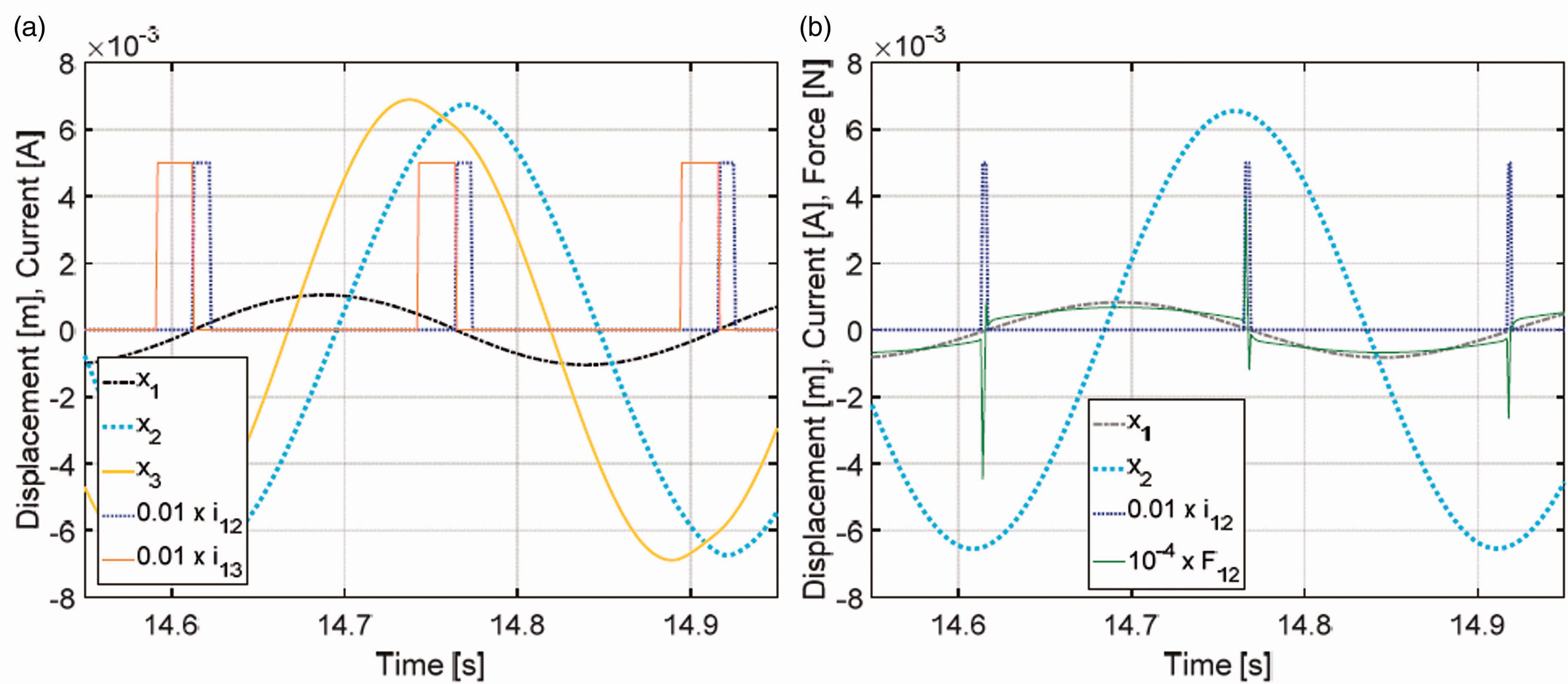
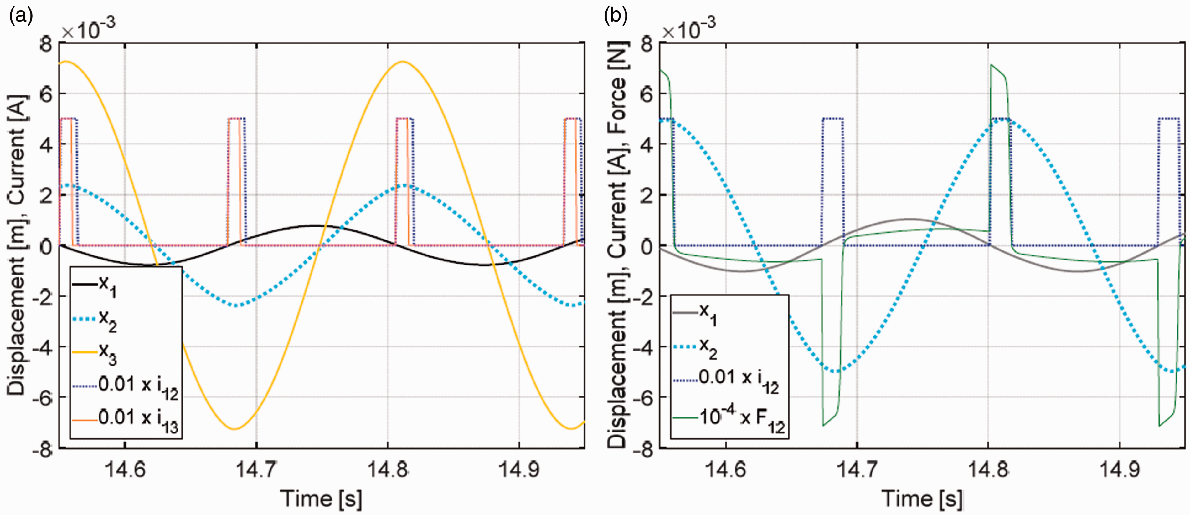
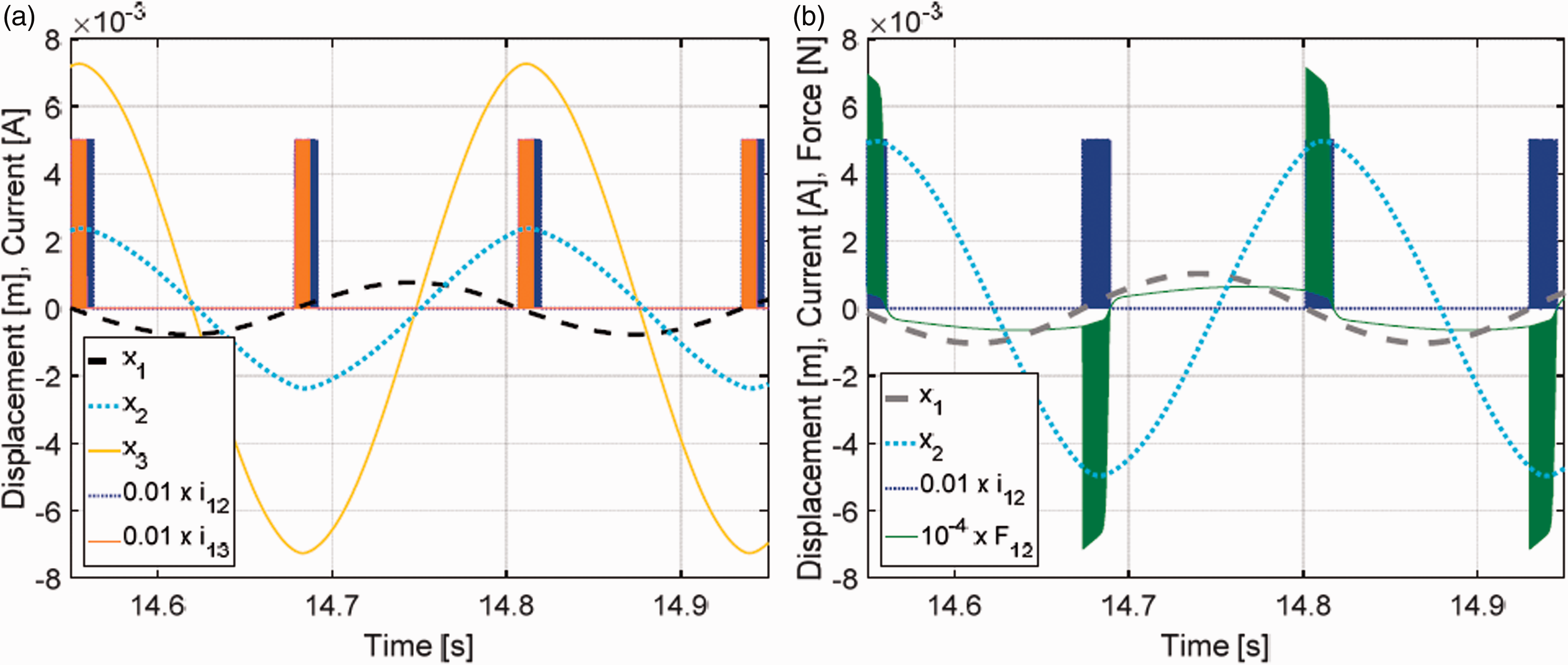
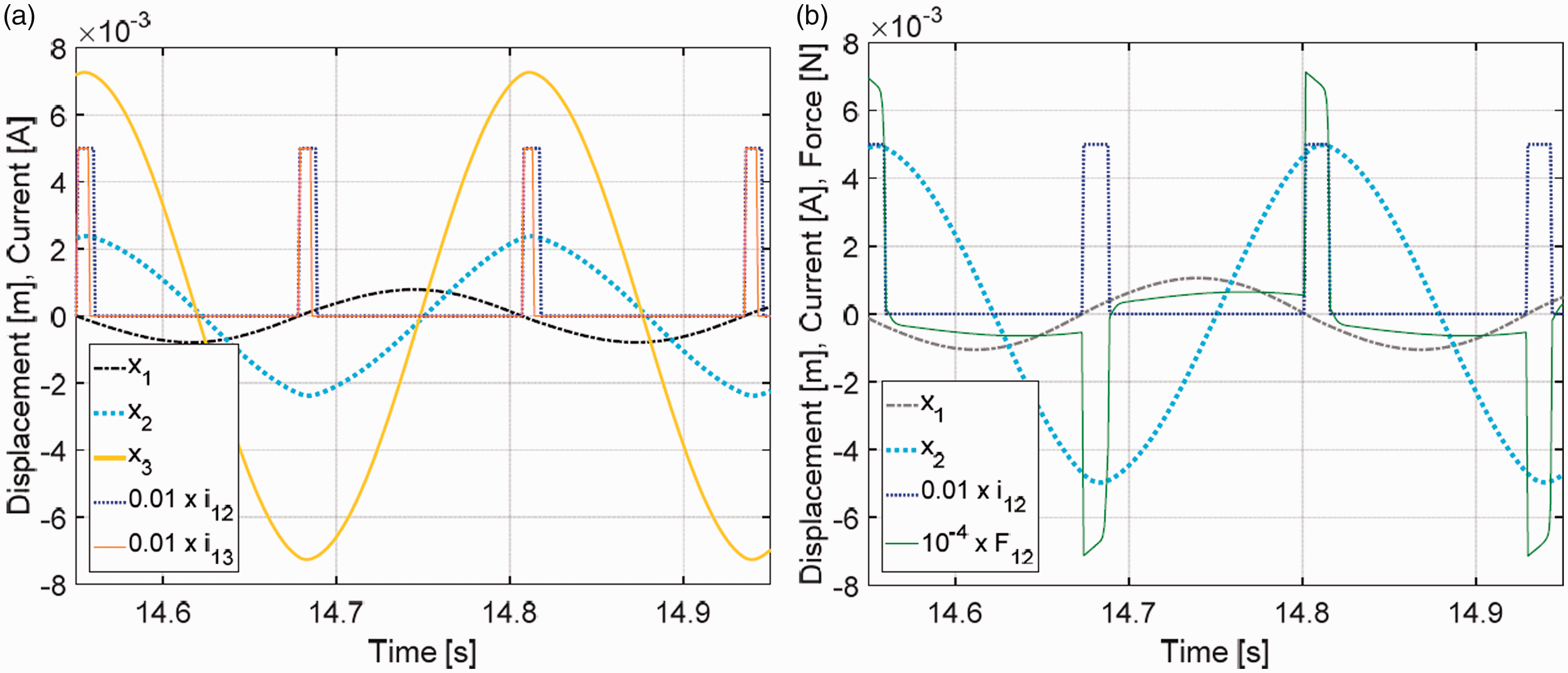
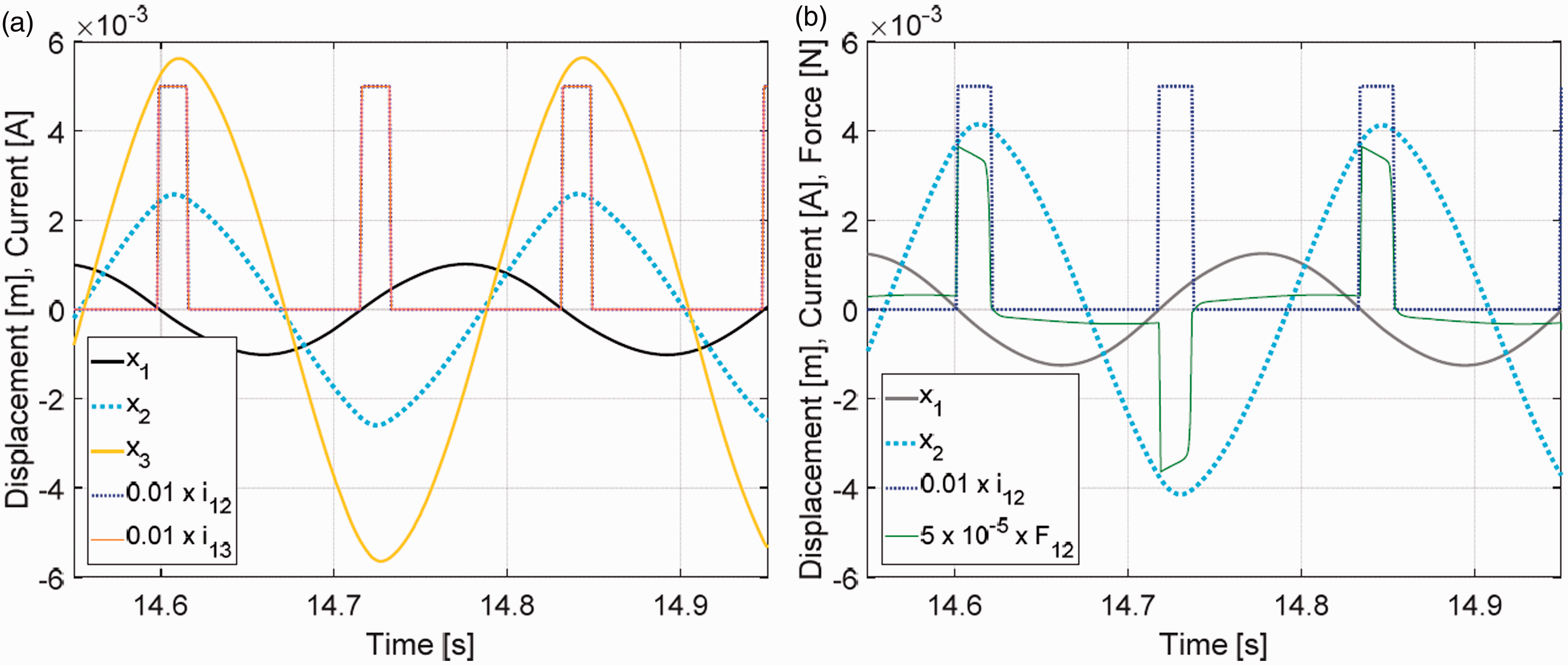
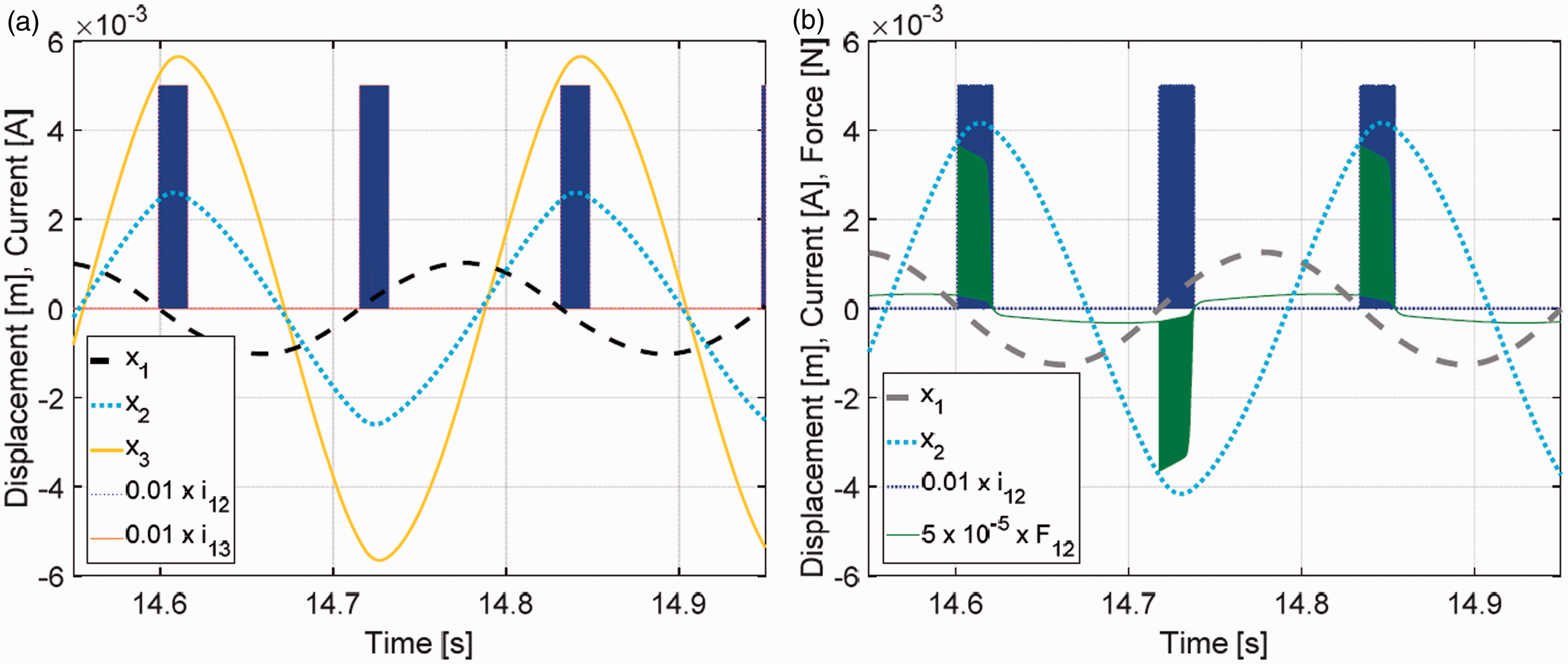
Figure 5 presents the comparison of DAFs for the Optimal control, Ground-Hook and Mod.GND law for the system with one and two MR TVAs. Figures 6 to 18 present the time patterns of $x_1$ , $x_2$ , $x_3$ , $i_{12}$ , $i_{13}$ obtained for the system with two MR TVAs (figure indices (a)) along with the time patterns of $x_1$ , $x_2$ , $i_{12}$ , and $\overline{F_{12}}$ for the system with one MR TVA (figure indices (b); ${\overline{MRD}}_{12}$ force is textualised as $F_{12}$ in figure legends for readability), for the Optimal control, Quasi-Optimal control, Mod.GND and the Ground-Hook law, at specific frequency points designated in Figure 4 as A (2.7 Hz), B (3.3 Hz), C (3.9 Hz) and D (4.3 Hz).

Figure 5.

Dynamic Amplification Factor (DAF) frequency characteristics: Optimal control vs. Ground-Hook vs. Mod.GND.

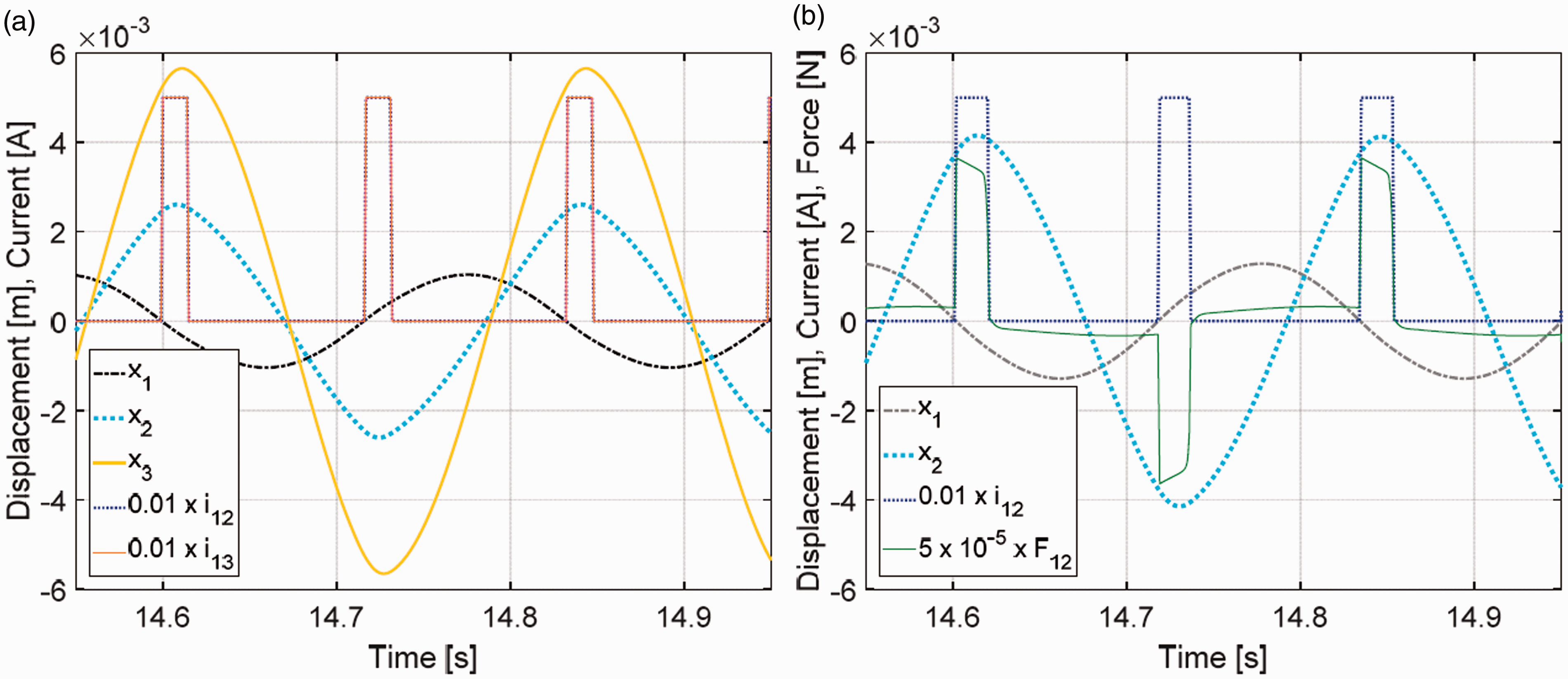
It may be observed (see Figure 6 vs. Figure 8, frequency point A, 2.7 Hz) that control current and force patterns generated by the Mod.GND law are a precise replication of the respective patterns of the Optimal control approach. Thus at frequency points B, C and D, the Mod.GND patterns are omitted (presented together with the Optimal control patterns). The same concerns frequency characteristics of the Optimal control and Mod.GND law (see Figure 5), thus they are determined separately but presented together in Figures 19 and 20 (the differences between the determined Optimal control and Mod.GND frequency characteristics are negligibly small). It is also evident (see Figure 4) that the frequency characteristics of the Optimal control and Quasi-Optimal control approaches are practically the same; however, the control patterns are different (but have the same envelopes) due to the high frequency co-state resetting to zero (and so high frequency zeroing of $i_{12}$ and $i_{13}$ ) for the Quasi-Optimal control approach. As it was mentioned earlier, the baseline Optimal and Quasi-Optimal (Q-O HF) approaches differ only at a countable number of samples when the co-state integrators are all reset to zero for the Q-O HF, and this makes no observable difference regarding vibration reduction results. There may be observed steeper edges of $i_{12}$ and $i_{13}$ patterns for the Quasi-Optimal control due to the smallert_s value adopted (see sections Baseline implementation technique and Alternative concepts).

Figure 6.

Time responses at 2.7 Hz (A), Optimal control: two (a), one (b) MR TVA.

Figure 7.

Time responses at 2.7 Hz (A), Quasi-Optimal control: two (a), one (b) MR TVA.

Figure 8.

Time responses at 2.7 Hz (A), Mod.GND: two (a), one (b) MR TVA.

It may be observed that using two passive TVAs instead of one, assuming the same total TVA mass (21.46 kg) and adequate stiffness/damping tuning, results in maximum DAF reduction by nearly 0.5, thus it may be considered reasonable. However, the utilisation of 2 MR TVAs instead of 1 MR TVA, assuming again the same total TVA mass, and the same total MR damper force limitations, seems questionable, as the 2 MR TVA solution is more sensor (displacement x₃, MR damper force F₁₃), data processing and calculation demanding, while the benefits are evident above the 3.6 Hz oscillation frequency only. Regarding the maximum DAF (and so $A(x_1)$ ) criteria, the 2 MR TVA solution advantage is minor.

Analysing the presented frequency characteristics and time patterns it may be concluded that the introduced Optimal control, Quasi-Optimal control and Mod.GND solutions are superior with regard to the passive TVA(s). The Ground-Hook law, in contrary to the Mod.GND approach, generates control current patterns resulting in force spikes of incorrect sign (at frequency points A and B, see Figure 9(b) and Figure 12(b)) or narrowed profiles of the maximum current (points C and D, Figures 15 and 18), that are different from the Optimal control/Mod.GND patterns, thus the Ground-Hook frequency characteristics (Figure 5) have noticeably higher values in wide frequency ranges than both the Optimal control and Mod.GND respective frequency characteristics.

Figure 9.

Time responses at 2.7 Hz (A), Ground-Hook: two (a), one (b) MR TVA.

Figure 10.

Time responses at 3.3 Hz (B), Optimal control/Mod.GND: two (a), one (b) MR TVA.

Figure 11.

Time responses at 3.3 Hz (B), Quasi-Optimal control: two (a), one (b) MR TVA.

Figure 12.

Time responses at 3.3 Hz (B), Ground-Hook: two (a), one (b) MR TVA.

Figure 13.

Time responses at 3.9 Hz (C), Optimal control/Mod.GND: two (a), one (b) MR TVA.

Figure 14.

Time responses at 3.9 Hz (C), Quasi-Optimal control: two (a), one (b) MR TVA.

Figure 15.

Time responses at 3.9 Hz (C), Ground-Hook: two (a), one (b) MR TVA.

Figure 16.

Time responses at 4.3 Hz (D), Optimal control/Mod.GND: two (a), one (b) MR TVA.

Figure 17.

Time responses at 4.3 Hz (D), Quasi-Optimal control: two (a), one (b) MR TVA.

Figure 18.

Time responses at 4.3 Hz (D), Ground-Hook: two (a), one (b) MR TVA.

Possible improvements

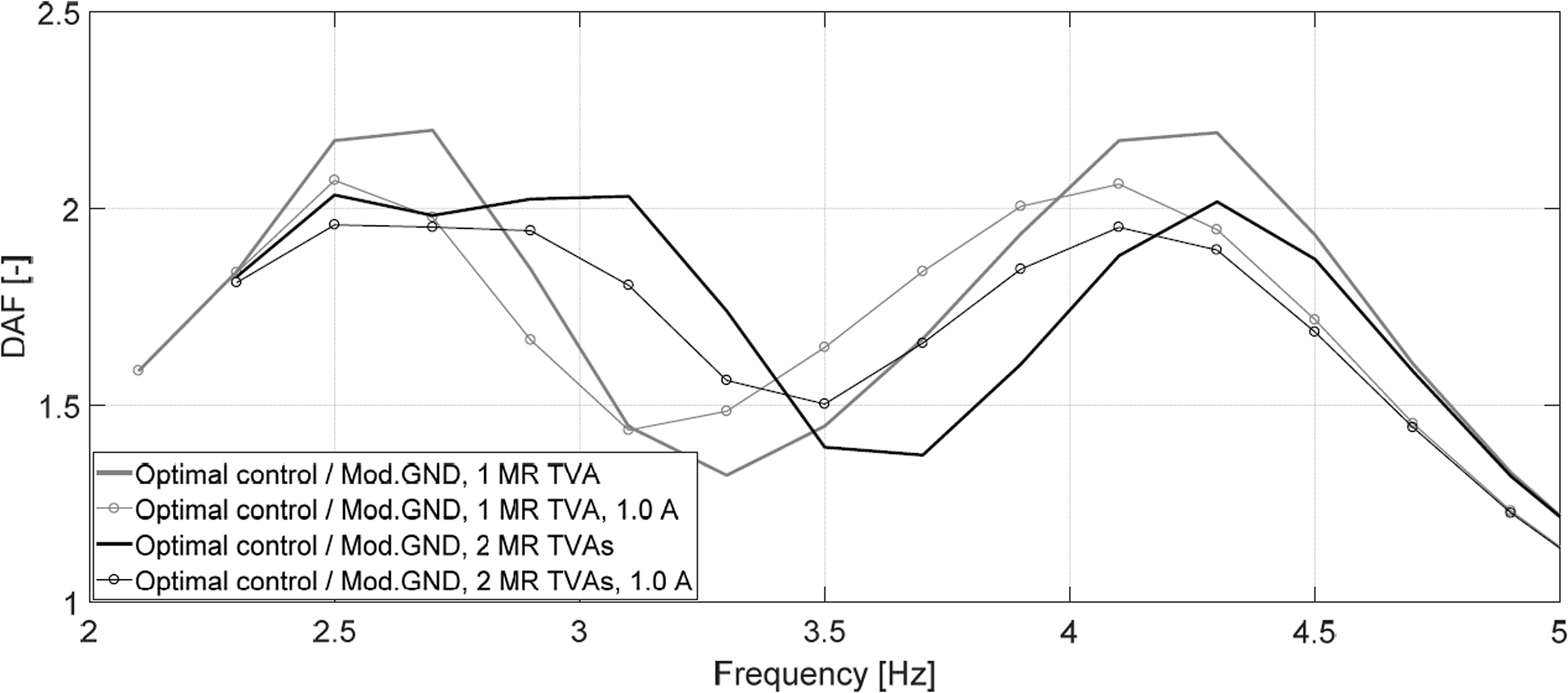
The results presented in the previous sections look encouraging. However, it was observed that further improvement is possible for the higher MR damper control current values. Assuming $i_{max}=1.0$ A, regarding the intermittent current limitation, ²¹ the frequency characteristics presented in Figure 19 are obtained.

Figure 19.

Dynamic Amplification Factor (DAF) frequency characteristics, Optimal control/Mod.GND: $i_{max}=0.5$ A (default here) vs. $i_{max}=1.0$ A.

Figure 19 shows a comparison of the frequency characteristics obtained for the Optimal control/Mod.GND law with 1 MR TVA and 2 MR TVAs assuming $i_{max}=0.5$ A or $i_{max}=1.0$ A. It may be observed that, in relation to $i_{max}=0.5$ A assumption, mainly right maxima are markedly lowered with $i_{max}=1.0$ A.

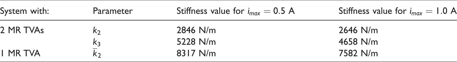
As the idea of the paper was to compare different approaches with one (or two) MR TVA(s), in relation to one standard passive TVA with ${\overline{k}}_2$ , ${\overline{c}}_2$ values set according to Den Hartog ¹⁶ (or two passive TVAs with k₂, k₃, c₂, c₃ values tuned accordingly to obtain the maxima of the DAF frequency characteristics of equal/lowest values), thus ${\overline{k}}_2$ (k₂ and k₃) value(s) was (were) maintained during all the simulation tests presented in Figures 6 to 18 (b) (Figures 6 to 18(a); information in the brackets concerns the 2 MR TVA system). However, each of the described control solutions exhibits a substantially higher left maximum of the frequency characteristics, than the right one. To lower that (the left) maximum and obtain equality of all the local maxima, passive spring(s) stiffness may be tuned, i.e. lowered. That is more crucial for the operation with 2 MR TVAs or/and $i_{max}=1.0$ A. To depict the control potential, values of ${\overline{k}}_2$ (k₂ and k₃) were optimised with regard to the equality and minimisation of the frequency characteristics maxima separately for the one- and two-TVA system, for $i_{max}=0.5$ A and $i_{max}=1.0$ A. The results are presented in the Table 2 and Figure 20. The values of m₁, c₁, m₂, ${\overline{m}}_2$ _, m₃ are kept unchanged (c₂, ${\overline{c}}_2$ and c₃ are not used here).

Figure 20.

Dynamic Amplification Factor (DAF) frequency characteristics, Optimal control/Mod.GND: $i_{max}=0.5$ A (default here) vs. $i_{max}=1.0$ A; k₂, k₃, ${\overline{k}}_2$ values optimised (see Table 2).

Table 2.

Optimised k₂, k₃ and ${\overline{k}}_2$ stiffness parameters.

System with:	Parameter	Stiffness value for $i_{max}=0.5$ A	Stiffness value for $i_{max}=1.0$ A
2 MR TVAs	k 2	2846 N/m	2646 N/m
	k 3	5228 N/m	4658 N/m
1 MR TVA	${\overline{k}}_2$	8317 N/m	7582 N/m

Figure 20 shows that using $i_{max}=1.0$ A constraint, almost 50% reduction of DAF (and so the maximum amplitude of $x_1$ ) is possible with regard to the respective passive 1 TVA/2 TVA solutions (compare with Figure 4). Even if 1.0 A maximum current setting is unavailable due to the high duty cycle (resulting in the MR damper possible overheating), the primary system (structure) maximum displacement amplitudes obtained for $i_{max}=0.5$  A are reduced more than 40% with regard to the respective passive system amplitudes maxima. The implementation of the 2 MR TVA system instead of the 1 MR TVA seems more reasonable for the optimised stiffness values, regarding the primary system (structure) displacement amplitude (and DAF) maximum rather than its full frequency profile.

Conclusions

The aim of this research was to develop and investigate several nonlinear vibration control concepts, including the online implementation of the one-step optimal control, computationally less demanding quasi-optimal control, and simple yet reliable optimal-based modified ground-hook law, in relation to the standard ground-hook and passive solutions with one and two MR TVAs. Three of the proposed algorithms proved their efficiency in vibration reduction within a wide frequency range, including almost 50% reduction of DAF with regard to the respective optimally tuned passive 1 TVA/2 TVA configurations (assuming a 1.0 A intermittent MR damper current constraint ²¹ ). Determination of the oscillation frequency for the MR TVA demanded stiffness/damping/friction calculation or for the algorithm parameters tuning is not necessary, thus online and real-time control implementation during transient, polyperiodic or random vibration phases is possible (which is not the case for many other solutions that have to switch to the passive mode during such phases). No offline calculation, nor excitations or disturbances assumption is necessary, both essential for continual online/real-time control.

The proposed Quasi-Optimal control method may save large computational load and its vibration control results are credible (as good as for the Optimal control), but sampling frequency has to be of the order of ${10}^4÷{10}^5$  Hz to cope well with the terminal condition (5) error (slight performance degradation is observed for the sampling rate of ${10}^3$ Hz); piecewise quasi-optimality is assumed here. The modified two-level displacement ground-hook law (Mod.GND) is indeed the simple implementation of the optimal control for the case when only the primary system/structure displacement amplitude has to be minimised. However, the proposed (one-step) Optimal control and Quasi-Optimal control solutions are more general, as the adopted quality index may encompass minimisation of, e.g., the MR damper stroke or velocity, the primary structure acceleration, or the actuator(s) effort (the MR damper force or control current). The experimental, real-time verification of the proposed methods, along with the investigation of the influence of the expanded quality index elements values on the vibration control quality, using a specially developed and built wind turbine tower-nacelle laboratory model equipped with single MR TVA, is presented in Martynowicz. ⁶²