Sage Journals: Discover world-class research

Abstract

This paper uses the Barycentric Lagrange interpolation method to explore the free vibration of a plate with the regular and irregular domain using the Chebyshev function, allowing us to consider multiple dimensions. From our results, it can be shown that the Barycentric Lagrange interpolation method can solve three-dimensional problems. In the analysis, we can see that the Barycentric Lagrange interpolation method can solve the dynamic motion of the plate with regular domain, and the error of the simulation can be reduced to 0.15%. The effect of the geometric node number on the simulated error of the natural frequency of the plate is very profound. The Barycentric Lagrange interpolation method and the extrapolation difference method can solve the natural frequency of the plate with irregular domain. The error of the simulation on the natural frequency can be reduced to 1.084%. This allows us to understand the vibration of the plate with the regular and irregular domain under various boundary conditions quickly.

Keywords

Vibration plate meshless Barycentric Lagrange interpolation irregular

Introduction

Numerical analysis is a very important tool to apply prediction to engineering problems. Many numerical methods are used to analyze various problems. Well-established tools include the finite element method and the finite volume method, available in business software. The finite volume method is used to solve fluid problems mainly, while the finite element method is mostly used to solve solid problems. Thus, the two methods must be chosen based on the state of the element. The property and shape of the element can affect the solution and convergence of the problem. In recent years, many researchers have started using meshless methods to solve engineering problems. The advantage of meshless methods is that they do not consider the state, just the node position and numbers.

There are many styles of meshless methods, though they share a common property of a need for a trial function and weight function. From the literature, the core of the meshless method is the trial function. Therefore, the trial function defines various meshless methods. There are the smooth particle method, moving least square, reproducing kernel particle method, point interpolation method, the partition of unity method, and the barycentric interpolation collocation method. The advantage of meshless methods is that we need not concern ourselves with the state of the elements, only node position. Therefore, we choose to use a meshless method to consider the vibrations of a plate. From the Chen and Wang¹ research result, we see that the high-accuracy Barycentric Lagrange interpolation can solve the biharmonic equation. This is used to solve the problem according to Ben et al.² The solution error of the problem can be reduced to 10⁻⁸. Thus, the numerical solution is very close to the solution by analysis. Lin et al.³ use this particular solution method to solve the problem of plate vibration. It solved the eigenvalue problem of the plate well enough, but did not solve the two-dimensional boundary value problem or the initial value problem.

The barycentric interpolation collocation method is based on the collocation point type, including the interpolation function. The interpolation method is a very powerful and widely applicable method. From the referenced article,⁴ we see that this includes the Lagrange interpolation method, the piecewise linear interpolation method, the spline interpolation method, and the rational function interpolation method. However, the equidistance nodes of geometric space can cause an unstable solution. In recent years, many researchers have used alternative methods to consider this problem, such as utilizing the Chebyshev function to construct the node position. This is not the equidistance node of geometric space, so it can improve the stability of our solution. Therefore, this paper uses the Chebyshev function to determine node position. From the literature, we know that the Chebyshev function used in conjunction with a meshless method can solve many classic engineering problems. This paper uses Lagrange interpolation in conjunction with the Chebyshev function to solve the two-dimensional boundary value problem and the initial value problem.

Then, the boundary value problem in irregular domain is very popular. The Chebyshev polynomials method and the base on the polynomials functions method have been applied to solve the boundary value problem in the irregular domain. Kong and Wu⁵ used the Chebyshev tau meshless method (CTMM) to solve boundary value problems that included curved boundaries. Based on their analysis, the CTMM is effective for solved Poisson-type problems in irregular domains.

Then, Shao and Wu⁶ combined the Fourier spectral method and the differential quadrature method in barycentric form to set up a numerical method to get the solution of the problems of thin plates resting on Winkler foundations with irregular domains. Shao et al.⁷ used the Chebyshev tau meshless method based on integration–differentiation (CTMMID) for numerically solving bi-harmonic-type equations in irregular domains with complex boundary conditions. Then, Shao and Wu⁸ use the Chebyshev tau meshless method (CTMM), which was based on the highest derivative, that solved the fourth-order equations in irregularly shaped domains with complex boundary conditions. In 2015, Shao and Wu⁹ combined the CTMMID with the domain decomposition method and applied it to solve the fourth-order problem on irregular domains. This circumvented the ill-conditioning problem.

According to the aforementioned studies, the meshless method can be used to get the approximate solution of the boundary value problem. The Chebyshev polynomial method can be applied to solve the approximate solution of plate deformation and can address the complex boundary condition, the regular domain and irregular domain, and high-derivative equations. The initial value problem with the regular domain and irregular domain by using the Chebyshev polynomial method cannot be found out in any literature. Therefore, this paper uses the meshless collocation method with barycentric rational interpolation to solve the vibration of a plate with the regular and irregular domain. The irregular domain can be applied to any shape. Then, this can solve the vibration problem of the plate with an irregular domain.

Theory

We will use the Lagrange interpolation method to solve the vibration of the plate. When we consider the one-dimensional problem with n + 1 nodes and the polynomial interpolation function, the solution is the polynomial function $p (x)$ . Therefore, the polynomial function can be shown as⁴

p (x) = \sum_{j = 1}^{n} L_{j} (x) f_{j}

(1)

where

L_{j} (x)

is the Lagrange interpolation base function. The Lagrange interpolation base function can be shown as

L_{j} (x) = \frac{Π_{k = 1, k \neq j}^{n} (x - x_{k})}{Π_{k = 1, k \neq j}^{n} (x_{j} - x_{k})}, j = 1, 2, 3…., n

(2)

From above equation, we can see that the property of the function is

L_{j} (x) = δ_{j k} = {\begin{matrix} 1, & j = k \\ 0, & j \neq k \end{matrix}

(3)

Considering the weight Lagrange interpolation, the weight function is

w_{j} = \frac{1}{\underset{j \neq k}{Π} (x_{j} - x_{k})}, j = 1, 2, …, n

(4)

Supposing the constant function is 1, whose interpolate is, of course, itself, we get

1 = \sum_{j = 1}^{n} L_{j} (x) f_{j}

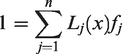
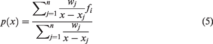
This gives us the barycentric formula for p

p (x) = \frac{\sum_{j = 1}^{n} \frac{w_{j}}{x - x_{j}} f_{i}}{\sum_{j = 1}^{n} \frac{w_{j}}{x - x_{j}}}

(5)

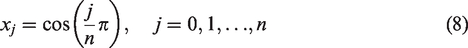
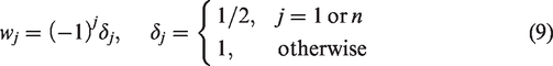
According to Chen and Wang,¹ these equidistant nodes are used to construct geometric space. However, Runge’s phenomenon can occur, causing an unstable solution. In order to account for the instability, we can choose the Chebyshev function to construct the node position. This will give us a stable solution. The first Chebyshev function is

x_{j} = \cos (\frac{2 j + 1}{2 n + 2} π), j = 0, 1, …, n

(6)

where the weight value is

w_{j} = {(- 1)}^{j} \sin (\frac{2 j + 1}{2 n + 2} π), j = 0, 1, …, n

(7)

The second Chebyshev function is

x_{j} = \cos (\frac{j}{n} π), j = 0, 1, …, n

(8)

where the weight value is

w_{j} = {(- 1)}^{j} δ_{j}, δ_{j} = {\begin{array}{l} 1 / 2, & j = 1 or n \\ 1, & otherwise \end{array}

(9)

The Chebyshev node is applied on the [–1,1] domain. Therefore, all these sets of Chebyshev points on the interval [−1,1] are linearly transformed to [a, b]. The variable function is y = x(b–a)/2+(b + a)/2 on the interval [–1,1].

Suppose a function u(x), represented by a polynomial interpolation in Lagrange form

u (x) = \sum_{j = 1}^{n} L_{j} (x) u_{j}

(10)

Then the m derivatives of u(x) are

u^{(m)} (x) = \sum_{j = 1}^{n} L_{j}^{(m)} (x) u_{j}

(11)

Suppose $x = x_{i}$ , this gives

u^{(m)} (x i) = \sum_{j = 1}^{n} L_{j}^{(m)} (x_{i}) u_{j}

(12)

On the $x_{i}$ node, then this is $L_{j}^{(m)} (x_{i}) = D_{i j}^{(m)}$

As $x_{i} \neq x_{j}$ , it can be shown that

L_{j}^{(1)} (x_{i}) = \frac{w_{j} / w_{i}}{x_{i} - x_{j}}, j \neq i

(13)

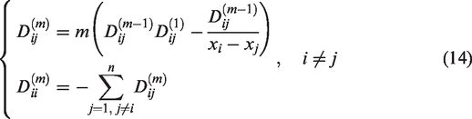
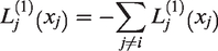
As for the case i = j, $1 = \sum_{j = 1}^{n} L_{j} (x) f_{j}$ implies $0 = \sum_{j = 1}^{n} L_{j}^{(m)} (x)$ for each differentiation order m and thus

L_{j}^{(1)} (x_{j}) = - \sum_{j \neq i} L_{j}^{(1)} (x_{j})

By using the collection method, we get the m-order differential function as

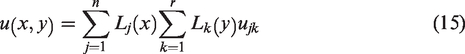
{\begin{cases} D_{i j}^{(m)} = m (D_{i j}^{(m - 1)} D_{i j}^{(1)} - \frac{D_{i j}^{(m - 1)}}{x_{i} - x_{j}}) \\ D_{i i}^{(m)} = - \sum_{j = 1, j \neq i}^{n} D_{i j}^{(m)} \end{cases}, i \neq j

(14)

The two-dimensional boundary value problem

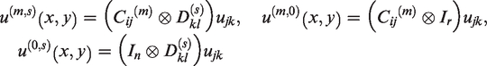
This considers the rectangular area [a,b]×[c,d]. The x line interval is [a,b]. The y line interval is [c,d]. The interval [a,b] is divided into n segments. The interval [c,d] is divided into r segments. This gives the two-dimensional function $u (x, y)$ . This is shown as

u (x, y) = \sum_{j = 1}^{n} L_{j} (x) \sum_{k = 1}^{r} L_{k} (y) u_{j k}

(15)

The m-order partial derivative $u (x, y)$ with respect to x is shown as

u^{(m)} (x, y) = \sum_{j = 1}^{n} L^{(m)}_{j} (x) \sum_{k = 1}^{r} L_{k} (y) u_{j k}

(16)

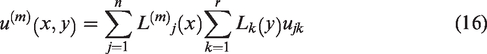
The s-order partial derivative $u^{(m)} (x, y) = \sum_{j = 1}^{n} L^{(m)}_{j} (x) \sum_{k = 1}^{r} L_{k} (y) u_{j k}$ with respect to y is shown as

u^{(m, s)} (x, y) = \sum_{j = 1}^{n} L^{(m)}_{j} (x) \sum_{k = 1}^{r} L^{(s)}_{k} (y) u_{j k}

(17)

where the

_{L}^{j} (x_{i}) = δ_{i j}

_{L}^{k} (y_{l}) = δ_{k l}

L_{j}^{(m)} (x_{i}) = C_{i j}^{(m)}

L_{k}^{(s)} (y_{l}) = D_{k l}^{(s)}

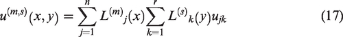
Therefore, this can be represented as

u^{(m, s)} (x, y) = (C_{i j}^{(m)} \otimes D_{k l}^{(s)}) u_{j k}, u^{(m, 0)} (x, y) = (C_{i j}^{(m)} \otimes I_{r}) u_{j k}, u^{(0, s)} (x, y) = (I_{n} \otimes D_{k l}^{(s)}) u_{j k}

where

\otimes

is the Kronecker product.

The two-dimensional boundary value and one initial value problem

This considers the rectangular area [a,b] × [c,d] and the time domain [e,f]. The time domain [e,f] is divided into h segments. The solution of the two-dimensional boundary value and one initial value problem is shown as

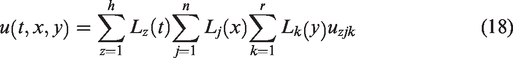
u (t, x, y) = \sum_{z = 1}^{h} L_{z} (t) \sum_{j = 1}^{n} L_{j} (x) \sum_{k = 1}^{r} L_{k} (y) u_{z j k}

(18)

Applying the same theorem, the m, s, and v partial derivatives with respect to x, y, and t, the equation is shown as

u^{(v, m, s)} (t, x, y) = \sum_{z = 1}^{h} L^{(v)}_{z} (t) \sum_{j = 1}^{n} L^{(m)}_{j} (x) \sum_{k = 1}^{r} L^{(s)}_{k} (y) u_{z j k}

(19)

where

_{L}^{j} (x_{i}) = δ_{i j}

_{L}^{k} (y_{l}) = δ_{k l}

L_{j}^{(m)} (x_{i}) = C_{i j}^{(m)}

L_{k}^{(s)} (y_{l}) = D_{k l}^{(s)}

L_{z}^{(v)} (t_{g}) = E_{z g}^{(v)}

_{L}^{z} (t_{g}) = δ_{z g}

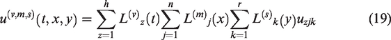
Therefore, this equation is

u^{(v, m, s)} (t, x, y) = [E_{z g}^{(v)} \otimes C_{i j}^{(m)} \otimes D_{k l}^{(s)}] u_{z j k}

(20)

u^{(v)} (t, x, y) = [E_{z g}^{(v)} \otimes I_{n} \otimes I_{r}] u_{z j k}

(21)

u^{(m, s)} (t, x, y) = [I_{h} \otimes C_{i j}^{(m)} \otimes D_{k l}^{(s)}] u_{z j k}

(22)

u^{(v, m)} (t, x, y) = [E_{z g}^{(v)} \otimes C_{i j}^{(m)} \otimes I_{r}] u_{z j k}

(23)

where

\otimes

is the Kronecker product.

The vibration problem of the plate

Considering the square plate, the geometry of the plate is [a,b]x[c,d]. From the governing equation of the plate, the dynamic function of the plate can be shown as¹⁰

\nabla^{4} u (t, x, y) + \frac{\partial^{2} u (t, x, y)}{\partial t^{2}} = 0

(24)

where

\nabla^{4} u (t, x, y) = \frac{\partial^{4}}{\partial x^{4}} + 2 \frac{\partial^{4}}{\partial x^{2} \partial y^{2}} + \frac{\partial^{4}}{\partial y^{4}}

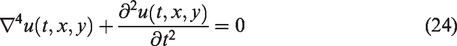
Therefore, the governing equation of the plate is shown as

\frac{\partial^{4} u (t, x, y)}{\partial x^{4}} + 2 \frac{\partial^{4} u (t, x, y)}{\partial x^{2} \partial y^{2}} + \frac{\partial^{4} u (t, x, y)}{\partial y^{4}} + \frac{\partial^{2} u (t, x, y)}{\partial t^{2}} = 0

(25)

Substituting the Barycentric Lagrange interpolation function, the dynamic function of the plate can be determined as

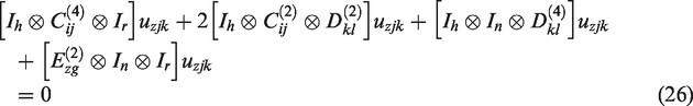
[I_{h} \otimes C_{i j}^{(4)} \otimes I_{r}] u_{z j k} + 2 [I_{h} \otimes C_{i j}^{(2)} \otimes D_{k l}^{(2)}] u_{z j k} + [I_{h} \otimes I_{n} \otimes D_{k l}^{(4)}] u_{z j k} + [E_{z g}^{(2)} \otimes I_{n} \otimes I_{r}] u_{z j k} = 0

(26)

We can rewrite the function as

[I_{h} \otimes C_{i j}^{(4)} \otimes I_{r} + 2 (I_{h} \otimes C_{i j}^{(2)} \otimes D_{k l}^{(2)}) + I_{h} \otimes I_{n} \otimes D_{k l}^{(4)} + E_{z g}^{(2)} \otimes I_{n} \otimes I_{r}] u_{z j k} = 0

(27)

The matrix form is depicted as

L U = 0

(28)

where

L = I_{h} \otimes C_{i j}^{(4)} \otimes I_{r} + 2 (I_{h} \otimes C_{i j}^{(2)} \otimes D_{k l}^{(2)}) + I_{h} \otimes I_{n} \otimes D_{k l}^{(4)} + E_{z g}^{(2)} \otimes I_{n} \otimes I_{r}, U = u_{z j k}

Boundary condition of the irregular domain

Clamp-supported condition

The boundary curve line of the irregular domain is discretized by taking m₀ nodes along the curved line ${(x_{K}^{b}, y_{K}^{b})}, K = 1, 2, 3 \dots, m_{0}$ . Therefore, the boundary condition function on the two-dimensional barycentric rational interpolation form can be expressed as

u (t, x_{K}^{b}, y_{K}^{b}) = 0 = \sum_{z = 1}^{h} L_{z} (t) \sum_{j = 1}^{n x} L_{j} (x_{K}^{b}) \sum_{k = 1}^{n y} L_{k} (y_{K}^{b}) u_{j k} = L_{1} U

(29)

\begin{array}{l} \frac{\partial u}{\partial n} (t, x_{K}^{b}, y_{K}^{b}) = [(\sum_{z = 1}^{h} L_{z} (t) \sum_{j = 1}^{n x} \frac{\partial L_{j} (x_{K}^{b})}{\partial x} \sum_{k = 1}^{n y} L_{k} (y_{K}^{b}) u_{j k}) n_{x} \\ + (\sum_{z = 1}^{h} L_{z} (t) \sum_{j = 1}^{n x} L_{j} (x_{K}^{b}) \sum_{k = 1}^{n y} \frac{\partial L_{k} (y_{K}^{b})}{\partial y} u_{j k}) n_{y}] = L_{2} U = 0 \end{array}

(30)

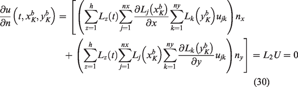
To ascertain the normal direction, the variable function of the curve line on the boundary of the irregular domain can be considered. If the boundary function is $Ø (x, y) = c$ , then the normal direction of the boundary curve can be expressed as

n = \frac{\nabla Ø}{| \nabla Ø |}

(31)

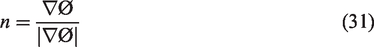
By combining the governing equation (28) and the boundary equation (31), this system matrix can be obtained as

[\begin{matrix} L \\ L_{1} \\ L_{2} \end{matrix}] U = [\begin{matrix} 0 \\ 0 \\ 0 \end{matrix}]

(32)

This matrix equation indicates that the node number on the calculative domain is nx × ny and the boundary node number is m₀. The $[\begin{matrix} L \\ L_{1} \\ L_{2} \end{matrix}]$ matrix is (nx × ny + m₀) × (nx × ny). The U matrix has (m × n) × 1 dimensions. Generally, the number of unknowns should be no fewer than the number of equations. Then, unknowns U can be determined using the least-squares method.

Numerical results

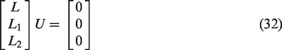
This considers a square plate of 1m×1m. A lateral force is applied to the plate of magnitude 1. In order to understand the deformation, the lateral force is a uniform force = 1. Every side of the plate is divided into 16 segments. Chebyshev points of the first kind are applied to construct the position of the node points, considering simple support on four sides of the plate. The analysis result can be shown in Figure 1. From analysis, this can give a maximum deformation of the plate of –0.0040625. The maximum deformation of Timoshenko and Woinowsky-Krieger¹⁰ is –0.00416. The error between maximum deformation of the paper and Timoshenko and Woinowsky-Krieger¹⁰ is about 2.34%.

Figure 1.

Deformation of plate with simple support under a lateral force = 1.

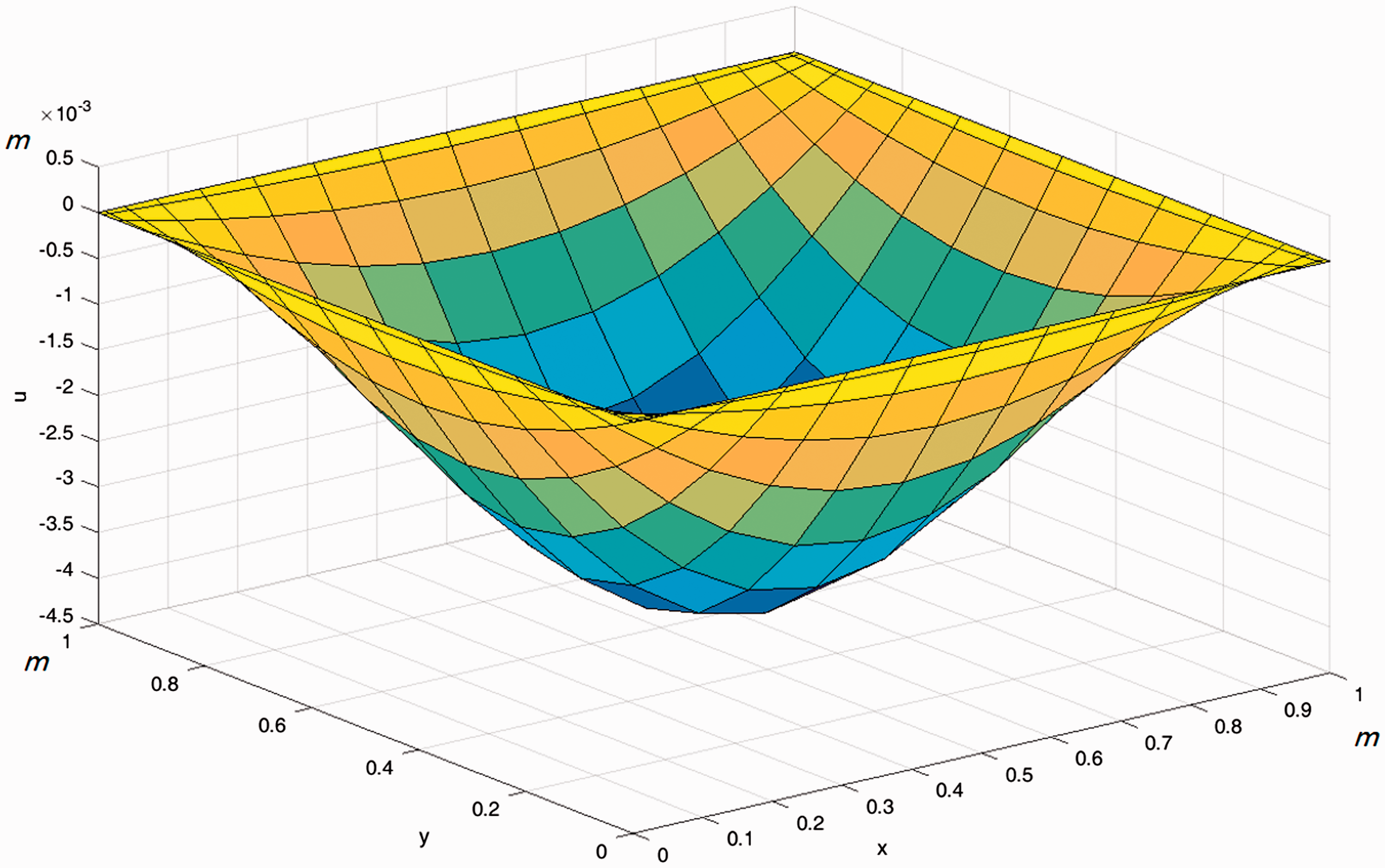
If the four sides of the plate are supported with clamps and the lateral force is 1, the maximum deformation of the plate under the same node numbers is –0.00125956. The maximum deformation of Timoshenko and Woinowsky-Krieger¹⁰ is –0.00126. The error between maximum deformation of the paper and Timoshenko and Woinowsky-Krieger¹⁰ is about 0.03492%. The deformation of the plate is shown in Figure 2.

Figure 2.

Deformation of plate with clamped support under a lateral force = 1.

Free vibration motion of the plate with the regular domain

In order to understand the free vibration of the plate, the initial deformation of the plate is calculated using a lateral uniform force = 1. When the lateral uniform force disappears, the motion of the plate creates a natural vibration. Therefore, the natural frequency of the plate under the variable condition can be determined. We must consider two conditions: simple support and clamped support.

Simple support condition

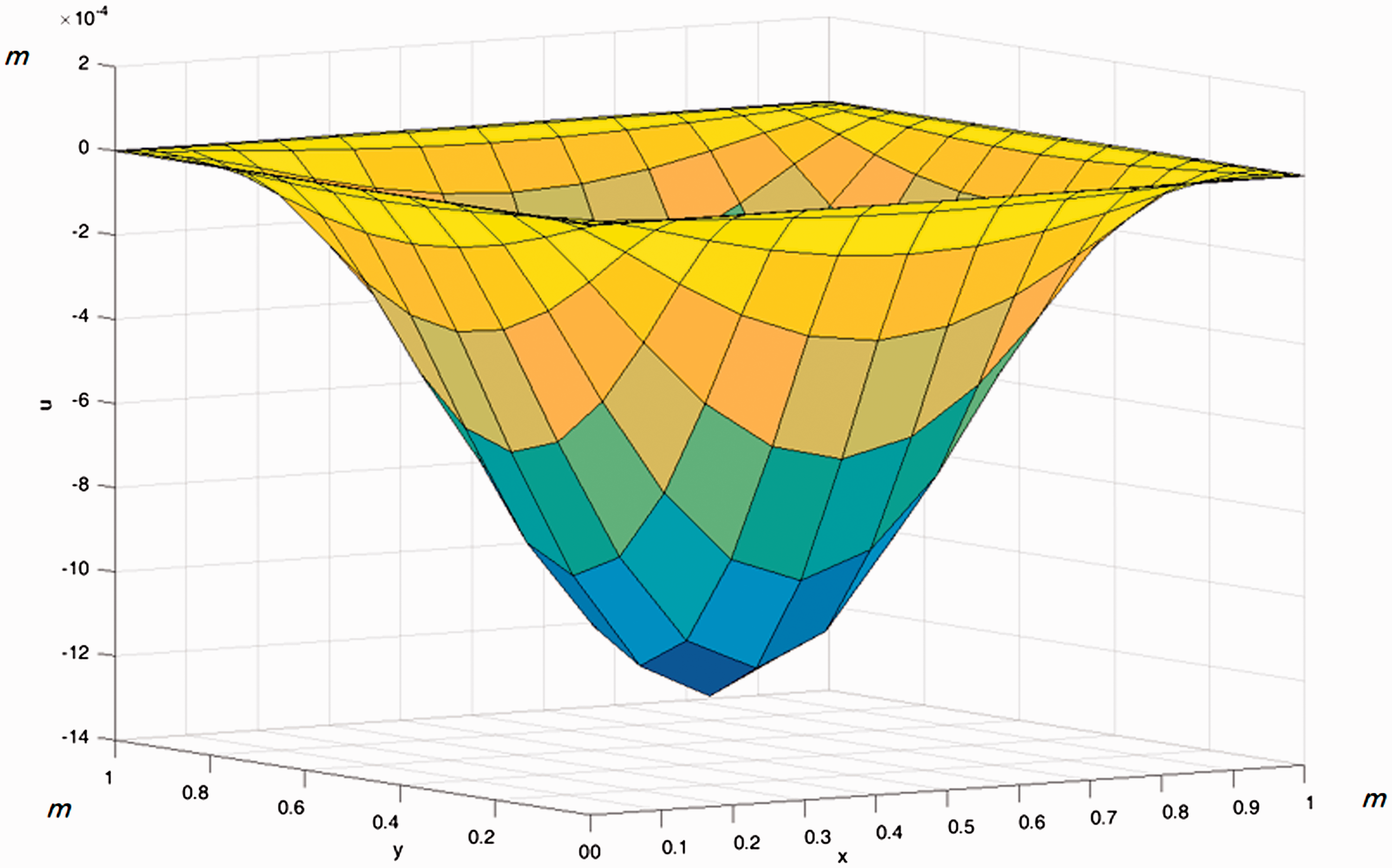
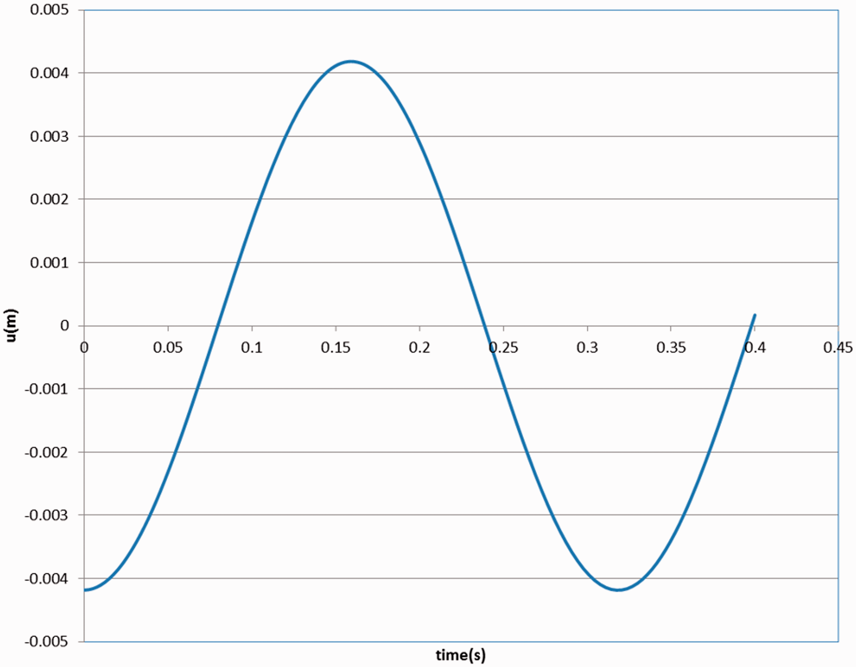
We will use a situation where every side of the plate is divided into eight segments, over a time interval of 0 to 0.4 s. Chebyshev points of the first kind are applied to construct a time node series with 40 time nodes. The large deformation of the plate is recorded, and the motion of the center point of the plate is shown in Figure 3. From Figure 3, we get a first natural frequency of the plate, under simple support conditions, of 19.9406. The first natural frequency of Timoshenko and Woinowsky-Krieger¹⁰ is 19.74. The error compared with Timoshenko and Woinowsky-Krieger¹⁰ is approximately 1.01%.

Figure 3.

Motion of the center of the plate over 40 time nodes.

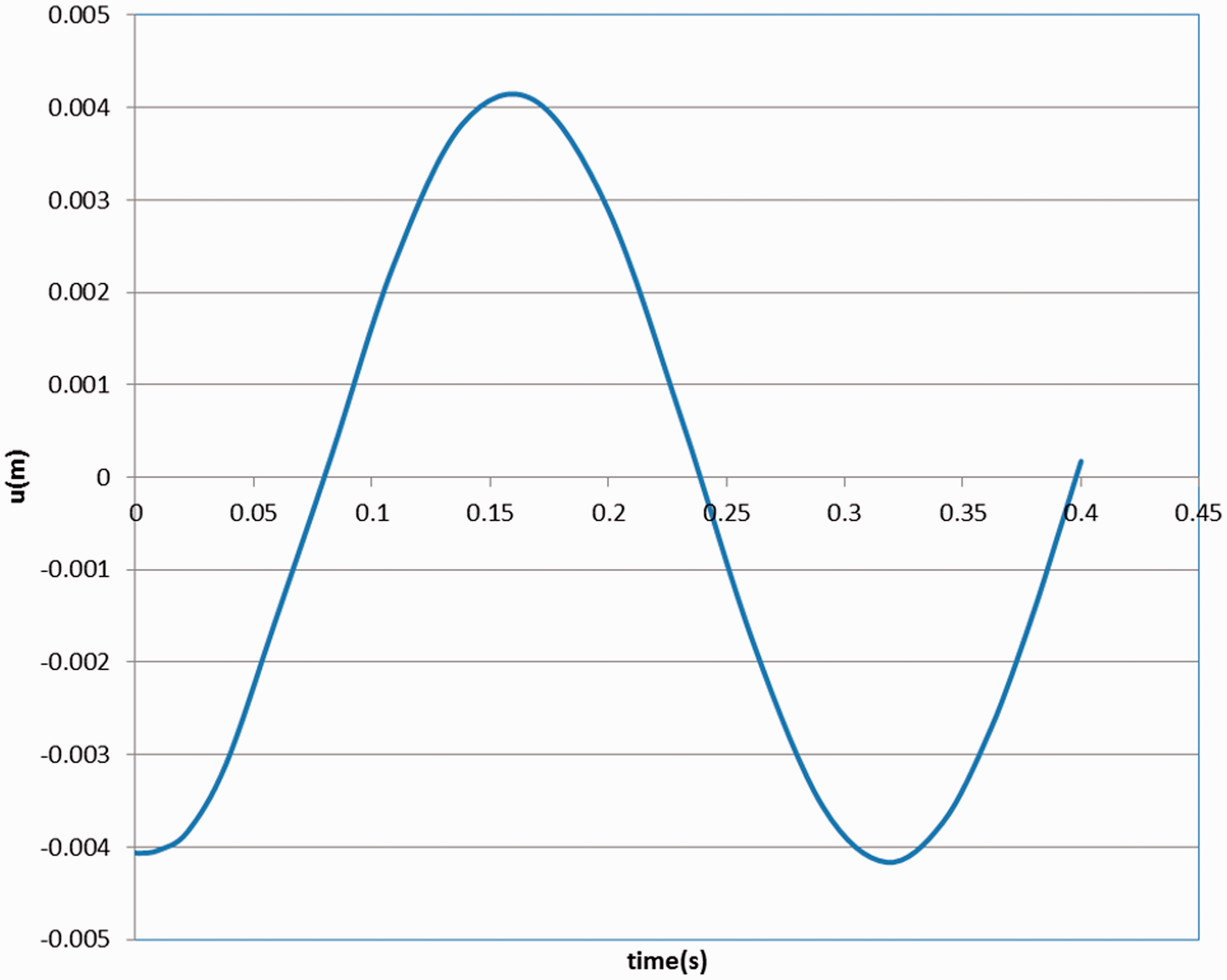
In order to understand the effect of the time domain node number on the solution accuracy, increase the number of time nodes to 80. The time interval is still 0 to 0.4 s, and every side of the plate is still divided into eight segments. The motion of the center point of the plate is shown in Figure 4. From Figure 4, we get a first natural frequency of the plate, under simple support conditions, of 19.55207. The first natural frequency of Timoshenko and Woinowsky-Krieger¹⁰ is 19.74. The error compared with Timoshenko and Woinowsky-Krieger¹⁰ is approximately 0.952%.

Figure 4.

Motion of the center of the plate over 80 time nodes.

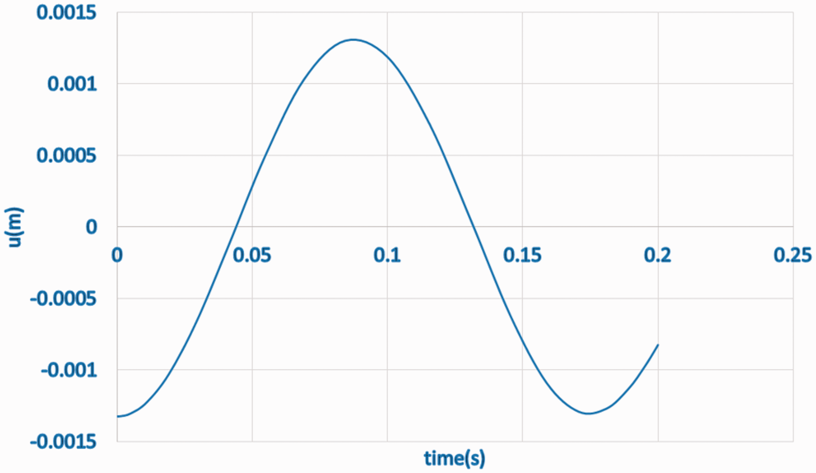
In order to understand the effect of the geometric node number on the solution accuracy, increase the number of dividing segments to 16. This causes a large node number, so decrease the number of time nodes to 20, still over the interval of 0 to 0.4 s. The motion of the center of the plate is shown in Figure 5. Analyzing this result, we get a first natural frequency of the plate of 19.786. The error compared with Timoshenko and Woinowsky-Krieger¹⁰ is about 0.23%. Thus, we can see that the effect of increasing the geometric node number increases the accuracy of our natural frequency calculations.

Figure 5.

Motion of the center of the plate over 20 time and 256 geometric nodes.

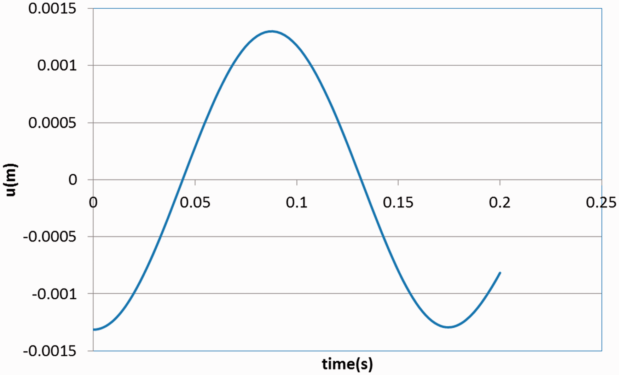
In order to understand the effects of the geometric node number and the time domain node number on solution accuracy, now calculate 16 segments and a time domain reduced to 0 to 0.2 s with 20 segments. The natural frequency of the plate, simply supported, is 19.786. When we reduce the time domain to 0 to 0.1 s with 20 segments, the natural frequency of the plate, simply supported, is still 19.786. From this result, we can know that great geometric and time node numbers can achieve a highly accurate solution.

Clamp support condition

We will use a situation where every side of the plate is fixed with four clamp support and divided into eight segments, over a time interval of 0 to 0.2 s with 20 nodes. Chebyshev points of the first kind are applied to construct the time node series and geometric node series. The large deformation of the plate is recorded, and the motion of the center point of the plate is shown in Figure 6. From Figure 6, we get a first natural frequency of the plate, under clamp support conditions, of 33.2267. The first natural frequency of Leissa¹¹ is 35.99. The error compared with Leissa¹¹ is approximately 7.68%.

Figure 6.

Motion of the center of the clamped plate, 64 geometric and 20 time nodes.

In order to get an accurate solution, consider a time interval of 0 to 0.2 s with 40 segments, still with the plate divided into eight segments. Chebyshev points of the first kind are applied to construct the time node series and geometric node series. The motion of the center point of the plate is shown in Figure 7. From Figure 7, we get a first natural frequency of the plate, under clamp support conditions, of 35.6918. The error compared with Leissa¹¹ is approximately 0.83%. Thus, our accuracy is greatly improved.

Figure 7.

Motion of the center of the clamped plate, 64 geometric and 40 time nodes.

If we increase the number of segments of the time domain to 60, we get a first natural frequency of the plate of 36.04511, shown in Figure 8. The error compared with Leissa¹¹ is now approximately 0.15%.

Figure 8.

Motion of the center of the clamped plate, 64 geometric and 60 time nodes.

Free vibration motion of the plate with an irregular domain

Clamp-supported circular plate

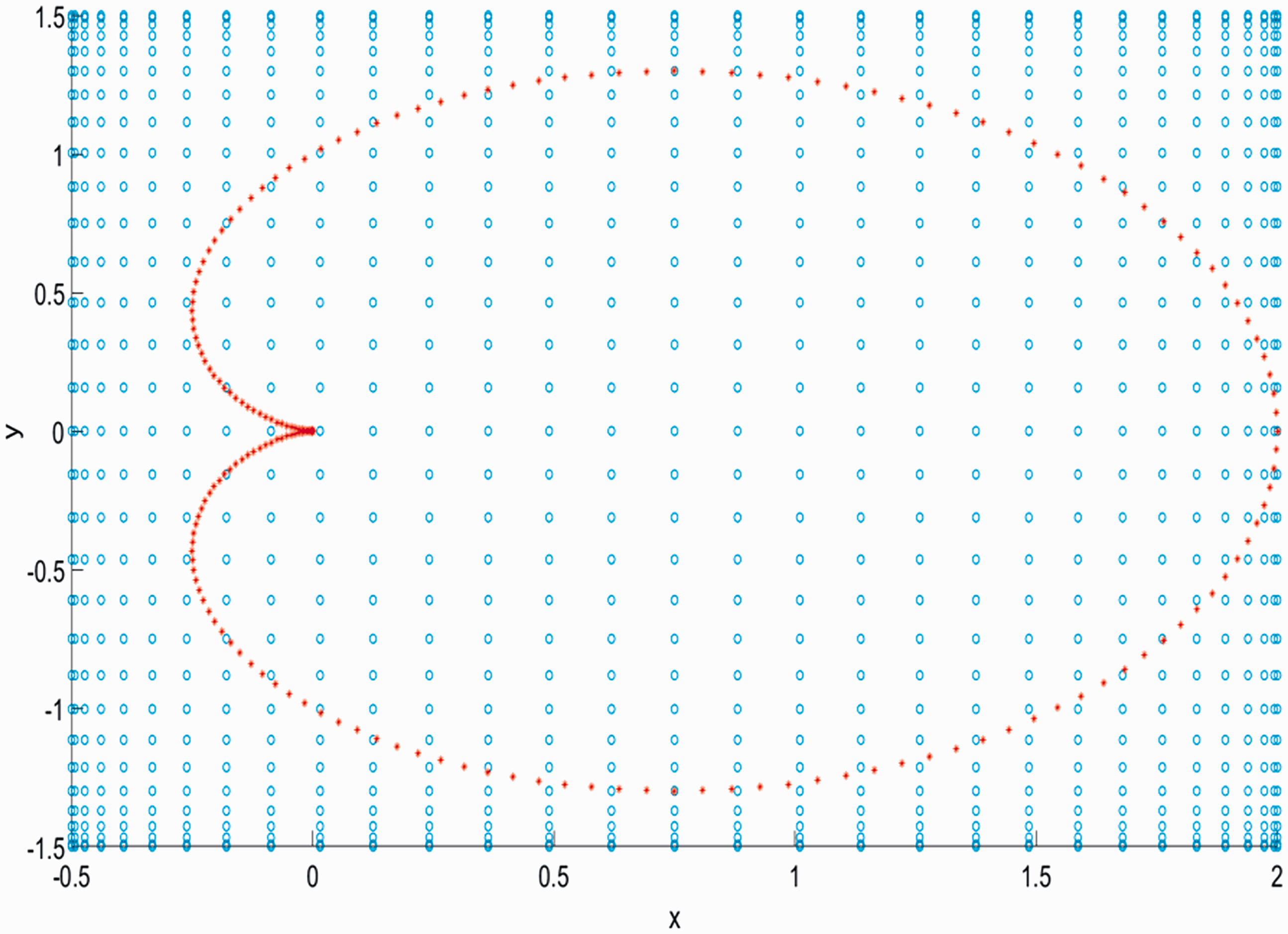
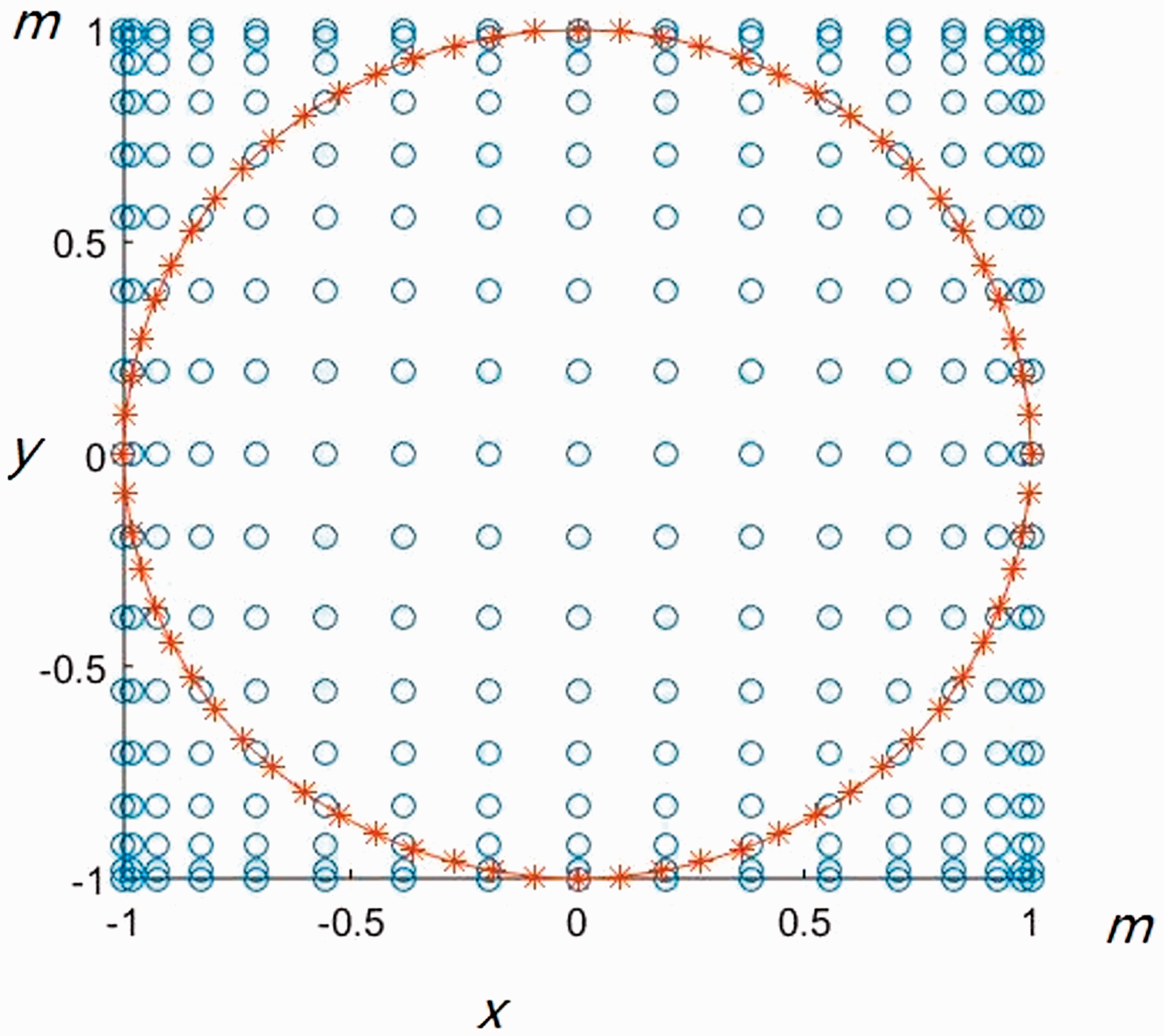
This example considers a circular plate with a clamp support. The domain of the circular plate is $Ω = {(x, y) : x^{2} + y^{2} < 1}$ . To fully embed it into the regular domain, the calculated regular domain is $Ω_{0} = {(x, y) : - 1 < x < 1, - 1 < y < 1}$ . This is depicted in Figure 9. Leissa¹² established that the node number of the embedding boundary must be greater than 2 × min(nx,ny)–1. The node number of the boundary curve is nx + ny. The circular boundary node number 68 is embedded in the 16 × 16 regular domain. This is depicted in Figure 9. The parameters of the plate are as follows: D = 1 and Poisson’s ratio μ = 0.3.

Figure 9.

Regular domain embedding circular boundary domain.

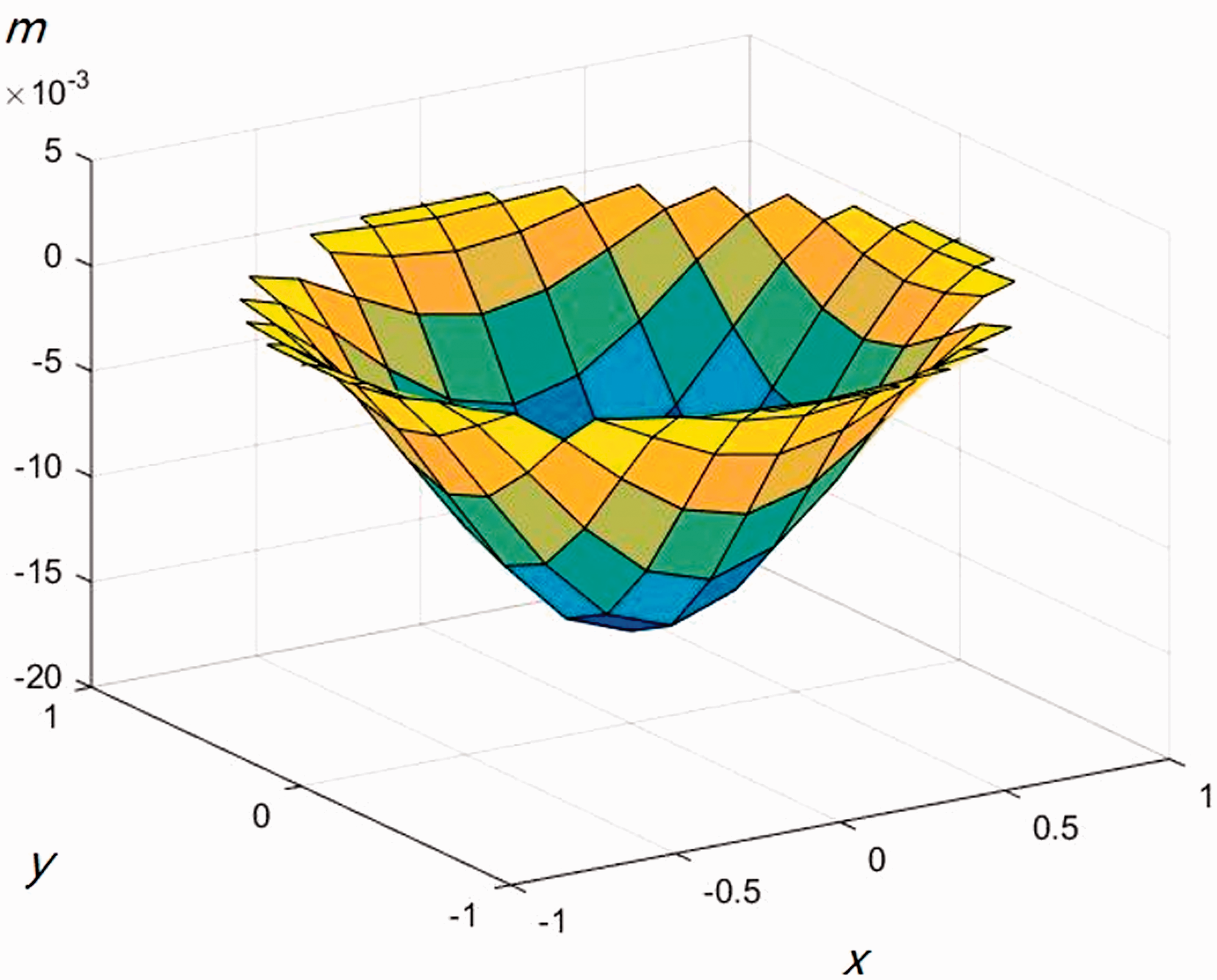
In order to get the initial shape of the plate in the natural vibration motion, the circular plate with clamp support and a uniform lateral load of f = 1 are considered. As this condition and load are applied, the center displacement of the circular plate is $\frac{f a^{4}}{64 D}$ .¹³ Here, the regular domain node number is 11 × 11, and the boundary node number is 22. The center displacement of the circular plate is –0.015625. The result is the same as the analytical solution. The initial shape of the plate is shown in Figure 10.

Figure 10.

Displacement of the circular plate with clamp support and lateral load f = 1 (regular domain 16 × 16).

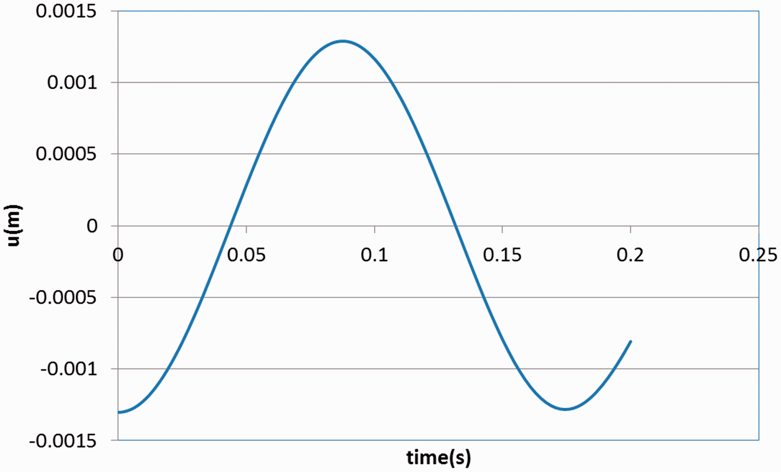
We will use a situation over a time interval of 0 to 0.8 s. Chebyshev points of the first kind are applied to construct a time node series with 30 time nodes. The large deformation of the plate is recorded, and the motion of the center point of the circular plate is shown in Figure 11. From Figure 11, we get natural period of vibration and a first natural frequency of the circular plate, under clamped-supported conditions, as 0.63367 s and 9.915538, respectively. The first natural frequency of the circular plate, under clamped-supported conditions of Leissa¹¹ is 10.2158. The error compared with Leissa¹¹ is approximately 2.9392%.

Figure 11.

Motion of the center of the circular plate over 30 time nodes.

From Figure 11, this can be known that the time nodes are discrete. This cannot get the accuracy result in the discrete time domain, directly. But, this can use the extrapolation difference method to get the high-accuracy result. By using the extrapolation difference method, the natural period of vibration and a first natural frequency of the circular plate, under clamped-supported conditions, are 0.62178 s and 10.10505, respectively. The error compared with Leissa¹¹ is approximately 1.084%.

Clamp-supported elliptical plate

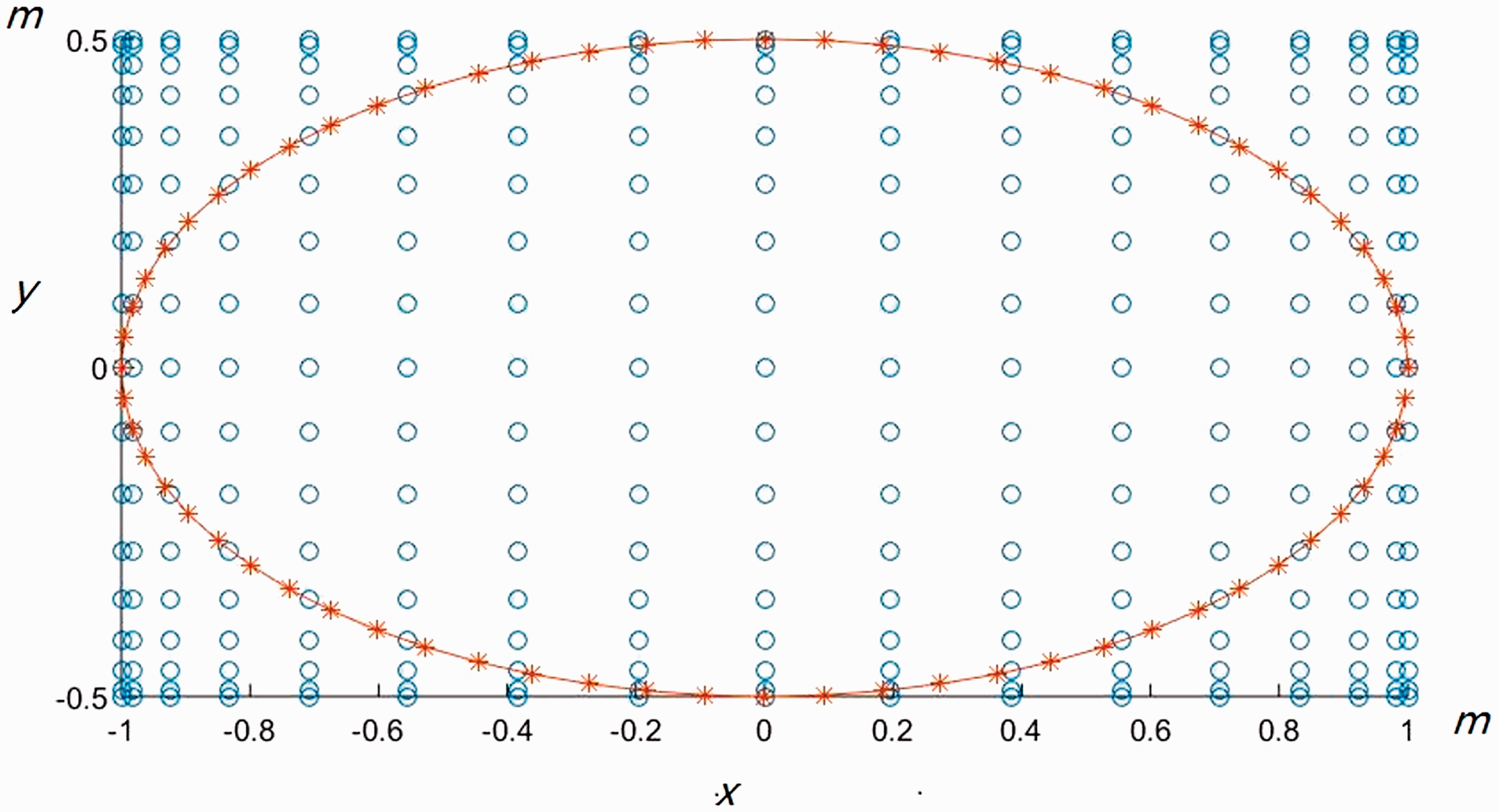
This example considers an elliptical plate with clamp support. The domain of the elliptical plate is $Ω = {(x, y) : \frac{x^{2}}{a^{2}} + \frac{y^{2}}{b^{2}} < 1}$ . To fully embed it into the regular domain, the calculated regular domain is $Ω_{0} = {(x, y) : - a < x < a, - b < y < b}$ . The calculated domain is 16 × 16; a = 1 and b = 0.5. The domain is depicted in Figure 12. The elliptical boundary node number 68 is embedded in the 16 × 16 rectangular domain. The parameters of the plate are D = 1.

Figure 12.

Regular domain embedding elliptical boundary domain.

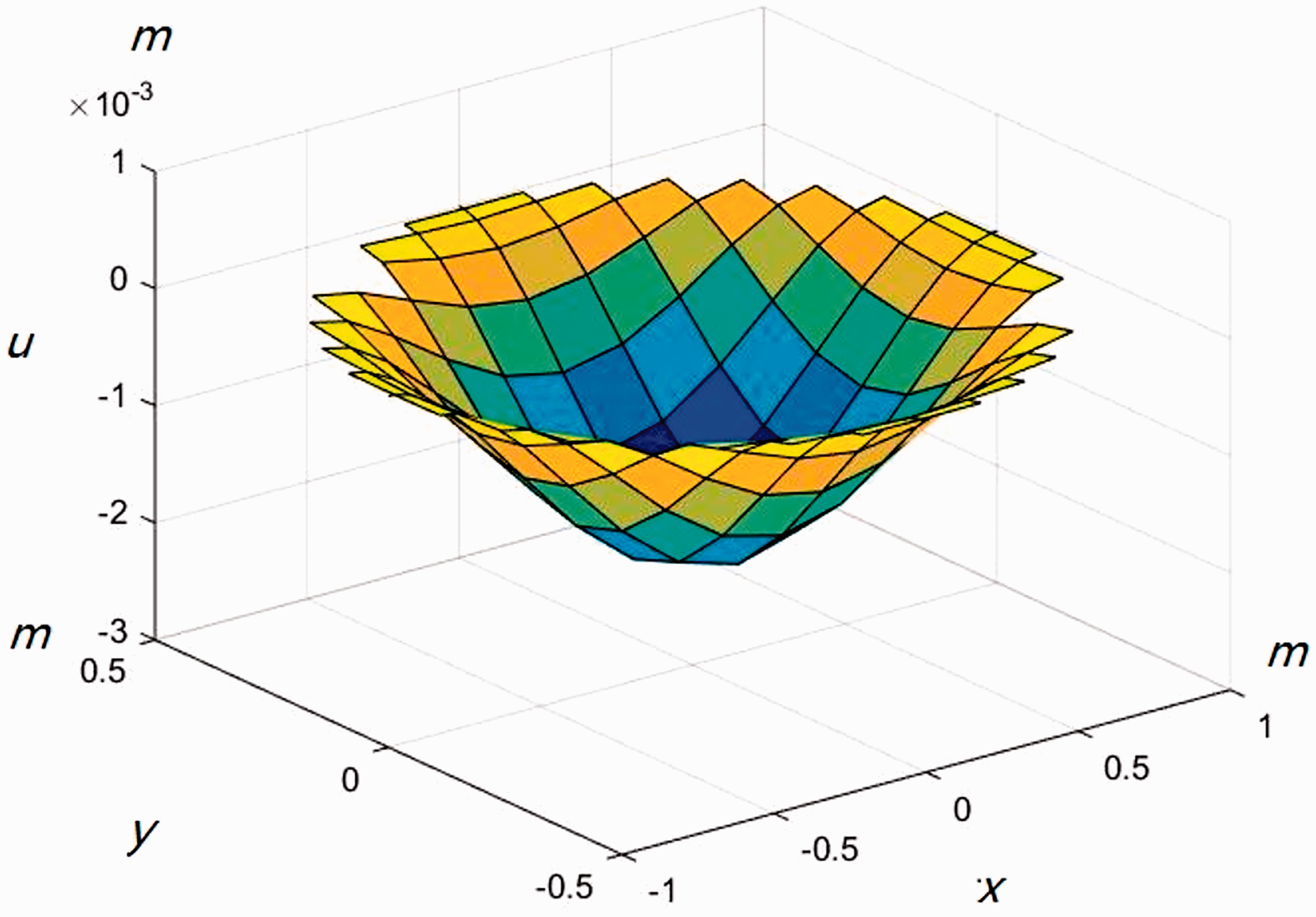
In order to get the initial shape of the plate in the natural vibration motion, the elliptical plate with clamp support and a uniform lateral load of f = 1 are considered. As this condition and load are applied, they yield a center displacement of the elliptical plate, that is, ${(\frac{24}{a^{4}} + \frac{24}{b^{4}} + 16 / (a^{2} b^{2}))}^{- 1}$ = –0.00211864.¹⁴ Now consider the regular domain node number 16 × 16 and the boundary node number 68. The center displacement of the elliptical plate is –0.00211864. The result is the same as the analytical solution. The initial shape of the plate is shown in Figure 13.

Figure 13.

Displacement of the elliptical plate with clamp support and lateral load f = 1 (regular domain 16 × 16).

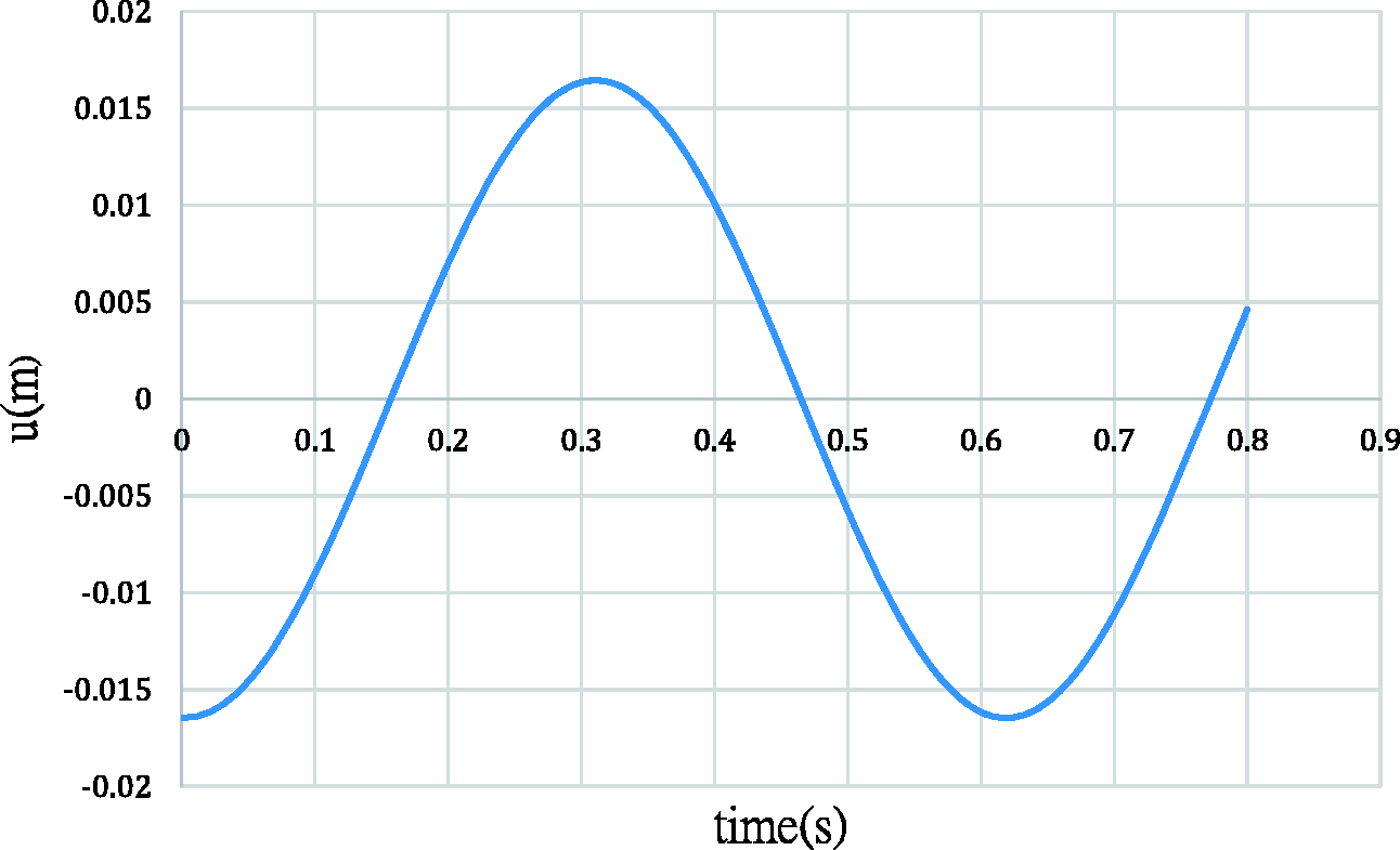
We will use a situation over a time interval of 0 to 0.4 s. Chebyshev points of the first kind are applied to construct a time node series with 50 time nodes. The large deformation of the elliptical plate is recorded, and the motion of the center point of the elliptical plate is shown in Figure 14. From Figure 14, we get natural period of vibration and a first natural frequency of the elliptical plate, under clamped-supported conditions, as 0.23095 s and 27.20587, respectively. The first natural frequency of the elliptical plate, under clamped-supported conditions of Leissa¹¹ is 27.5. The error compared with Leissa¹¹ is approximately 1.07%.

Figure 14.

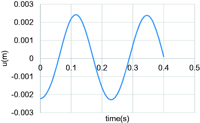
Motion of the center of the elliptical plate with clamp support over 50 time nodes.

Clamp-supported heart-shaped plate

This example considers the heart-shaped plate with clamp support. The domain of the heart-shaped plate is $Ω = {(r, θ) : 1 < 1 + \cos θ, 0 < θ < 2 π}$ . To fully embed it into the regular domain, the calculated regular domain is $Ω_{0} = {(x, y) : a < x < b, c < y < d}$ . The calculated domain is 30 × 30; a = –0.5, b = 2, c=–1.5, and d = 1.5. The domain is depicted in Figure 15. The heart-shaped boundary node number 124 is embedded in the 30 × 30 rectangular domain. The parameters of the plate are D = 1.

Figure 15.

Regular domain embedding elliptical boundary domain.

In order to get the initial shape of the heart-shaped plate in the natural vibration motion, the elliptical plate with clamp support and a uniform lateral load of f = 1 are considered. As this condition and load are applied, they yield a maximum displacement of the heart-shaped plate, that is, –0.030762 by using the ANSYS software. This is shown in Figure 16. Now, consider the regular domain node number 30 × 30 and the boundary node number 124. The center displacement of the heart-shaped plate is –0.031979. The result is very close to the ANSYS result. The initial shape of the plate is shown in Figure 17.

Figure 16.

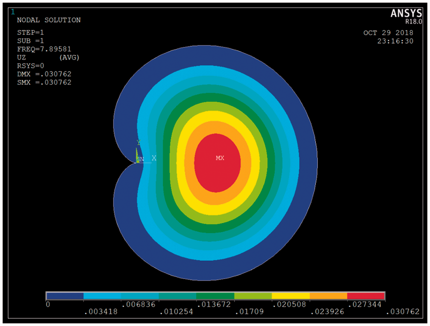
The first natural frequency and mode shape of the heart-shaped plate with the clamp-supported boundary condition in ANSYS software.

Figure 17.

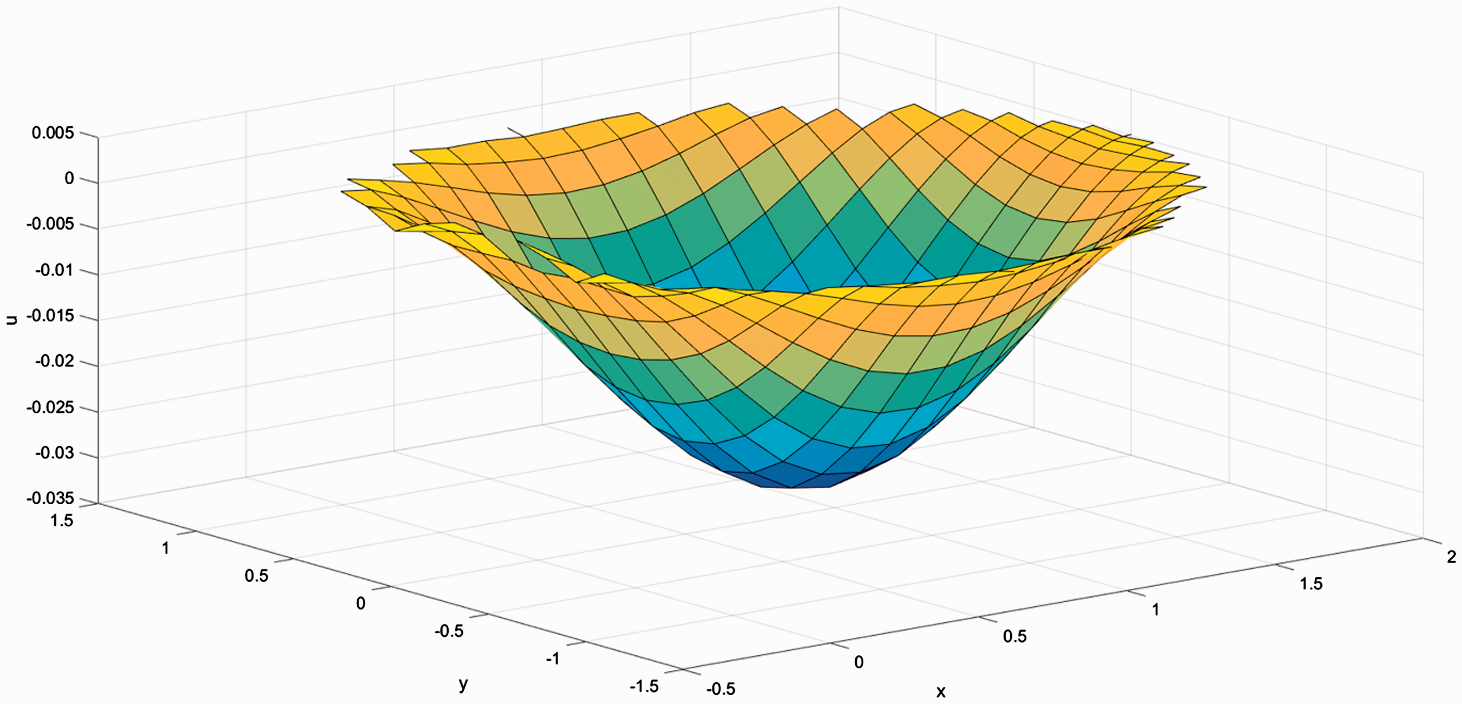
Displacement of the heart-shaped plate with clamp support and lateral load f = 1 (regular domain 30 × 30).

We will use a situation over a time interval of 0 to 0.4 s. Chebyshev points of the first kind are applied to construct a time node series with 10 time nodes. In order to reduce the computing time, the regular domain node number 8 × 8 is considered. We can get the first natural frequency of the heat-shaped plate, under clamped supported conditions, as 5.9997. The first natural frequency of the heat-shaped plate, under clamped-supported conditions, is 7.89581 by using the ANSYS software, as shown in Figure 16. The error compared with the result of the ANSYS is approximately 24.01373%. In order to reduce the analysis error, this also considers a aituation over a time inerval of 0 to 0.4s. The time nodes increases from 10 to 100 time nodes. We get a first natural frequency of the heart-shaped plate, under clamped-supported conditions, from 5.9997 to 7.822044. These errors compared with the result of the ANSYS are from 24.01373% to 0.934245%. This result is shown in Figure 18. From this result, it can be known that the high time node can reduce the error of the first natural frequency by using the Barycentric Lagrange interpolation method.

Figure 18.

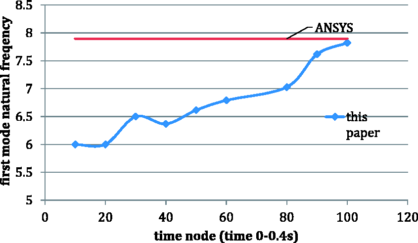
The first natural frequency and mode shape of the heart-shaped plate with the clamp-supported boundary condition under the variable time node (time 0–0.4 s).

Conclusion

This paper uses the Chebyshev function and Barycentric Lagrange interpolation method in conjunction to solve the dynamic motion of a vibrating plate with the regular and irregular domain. In order to get the natural frequency of the plate with the regular and irregular domain, we record the motion of the center point of a plate. From this analysis result, we can give the following conclusions:

This method can accurately calculate the natural frequency of the plate under various boundary conditions.

When considering high geometric node numbers, smaller time node numbers cause a greater numerical error.

The time node numbers determine an accurate solution of the free vibration of a clamped plate.

The embedding boundary curving method can be used to solve the vibration of the plate with an irregular domain.

When the Barycentric Lagrange interpolation method and the extrapolation difference method is applied simultaneously, this can increase the accuracy of the solution of the natural frequency of the plate.

Footnotes

Declaration of conflicting interests

The author(s) declared no potential conflicts of interest with respect to the research, authorship, and/or publication of this article.

Funding

The author(s) received no financial support for the research, authorship, and/or publication of this article.

References

Chen

Wang

High-accuracy barycentric interpolation collocation method – algorithms, program and applications. Beijing: China Science Publishing & Media Ltd, 2012.

Ben

Chorev

Croisille

IP.

A compact difference scheme for the biharmonic equation in planar irregular domains. SIAM J Numer Anal 2009; 49: 3087–3108.

Lin

Chen

Wang

, et al. Method of particular solutions using polynomial basis functions for the simulation of plate bending vibration problems. Appl Math Model 2017; 49: 452–469.

Berrut

Trefethen

NL.

Barycentric Lagrange interpolation. SIAM Rev 2004; 46: 501–517.

Kong

XH.

Chebyshev tau matrix method for Poisson-type equations in irregular domain. J Comput Appl Math 2009; 228: 158–167.

Shao

XH.

Fourier differential quadrature method for irregular thin plate bending problems on Winkler foundation. Eng Anal Bound Elem 2011; 35: 389–394.

Shao

Chen

SQ.

Chebyshev tau meshless method based on the integration–differentiation for biharmonic-type equations on irregular domain. Eng Anal Bound Elem 2012; 36: 1787–1798.

Shao

XH.

Chebyshev tau meshless method based on the highest derivative for fourth order equations. Appl Math Model 2013; 37: 1413–1430.

Shao

XH.

An effective Chebyshev tau meshless domain decomposition method based on the integration–differentiation for solving fourth order equations. Appl Math Model 2015; 39: 2554–2569.

10.

Timoshenko

Woinowsky-Krieger

Theory of plates and shells. 2nd ed. New York: McGraw-Hill, 1989.

11.

Leissa

AW.

Vibration of plates. Washington, DC: U.S. Government Printing Office, 1969.

12.

Wang

ZQ.

High-precision meshless collocation method with barycentric rational interpolation: algorithm, program and engineering application. China: Science Press, 2012 (in Chinese).

13.

Timoshenko

Woinowsky-Krieger

Theory of plates and shells. 2nd ed. New York: McGraw-Hill Book Company, 1959.

14.

Sergei

Brunello

Trefftz spectral method for initial boundary problems. Comput Assisted Mech Eng Sci 1997; 4: 549–565.

Vibration analysis of the plate with the regular and irregular domain by using the Barycentric Lagrange interpolation

Abstract

Keywords

Introduction

Theory

The two-dimensional boundary value problem

The two-dimensional boundary value and one initial value problem

The vibration problem of the plate

Boundary condition of the irregular domain

Clamp-supported condition

Numerical results

Free vibration motion of the plate with the regular domain

Simple support condition

Clamp support condition

Free vibration motion of the plate with an irregular domain

Clamp-supported circular plate

Clamp-supported elliptical plate

Clamp-supported heart-shaped plate

Conclusion

Footnotes

Declaration of conflicting interests

Funding

References