Sage Journals: Discover world-class research

Abstract

Low-frequency noise emitted by elevated viaducts in light rail transit lines has considerable adverse effects on inhabitants living nearby. Reliable prediction of the acoustic field radiating from the viaduct using forward numerical models is challenging because the model parameters that influence viaduct vibration are difficult to obtain. To avoid directly quantifying these parameters, such as wheel–rail combined roughness, an inverse method is presented to reconstruct the acoustic field using modal acoustic transfer vectors and the sound pressures at a small number of measurement points. First, a forward numerical method based on the train–track–bridge interaction analysis is performed to predict the structure-borne noise of a concrete box girder viaduct. Then, the calculated sound pressures are treated as virtual measurement results to illustrate the inverse method procedure. Both QR decomposition and singular value decomposition with Tikhonov regularisation are used in the inverse analysis. Third, the proposed inverse method is validated by comparing the sound pressure levels computed using the inverse method with the results simulated using the forward prediction method. Finally, the reliability of the inverse procedure is further validated through field tests of two U-shaped girder viaducts.

Keywords

Low-frequency noise concrete viaducts sound reconstruction inverse method noise prediction

Introduction

The overall noise level of a railway bridge system is usually larger than that of the ground track system, due to train-induced bridge vibration. Stiebel et al.¹ showed that the total noise levels of railway steel bridges with directly fastened track, steel bridges with ballasted track and concrete bridges with ballasted track could be 12 dB, 6 dB or 3 dB greater than plain track, respectively. Experimental and numerical results showed that concrete viaducts mainly generated low-frequency noise emissions (20–200 Hz),² which were easy to ignore when A-weighted sound pressure level (SPL) was utilised for evaluation. Low-frequency vibration and noise can cause annoyance, physiological disorders and sleep deprivation.^3–5 Moreover, low-frequency noise is difficult to control with traditional sound barriers. Thus, an efficient method is needed to study and attenuate low-frequency bridge noise.

A variety of forward prediction methods have been proposed to simulate bridge noise. First, bridge vibration can be obtained from the dynamic analysis of train–track–bridge interaction in the frequency domain^6,7 or time domain.^2,8 Then, various acoustic models can be applied to simulate sound pressure emitted by the bridge. Lee et al.⁹ simulated the sound radiation from a highway bridge using the Kirchhoff–Helmholtz integral. Oostdijk et al.¹⁰ used the concept of radiation ratio and empirical equations to predict the noise level of a steel-concrete railway bridge. Zhang et al.¹¹ used a hybrid finite element and statistical energy analysis method to simulate the sound pressure emitted from a concrete box girder with a simplified radiation model. A three-dimensional (3D) boundary element method (BEM) can be used to predict sound radiation from complex bridge structures.^2,12 The computation time and storage requirements needed for 3D BEM increase rapidly with the increase of the number of elements. To facilitate the acoustic analysis of bridge structures, a two-and-a-half-dimensional (2.5D) BEM-based procedure was developed in our previous work.¹³ The 2.5D method can be utilised to compute the solution of a 3D model with an invariant section using a spatial Fourier transform of the related 2D solutions.^13–15 However, due to the uncertainty of the model parameters used in forward simulation, predicting the absolute levels of the acoustic field is quite difficult. For instance, the damping and stiffness of the rail fastener and rail pad, and the combined wheel–rail roughness, are difficult to measure directly and accurately during railway operation. For this reason, the predicted results in earlier works^6–12 only agreed with the measured results for some field points and specific frequencies, while for other field points and frequencies, the predicted values achieved less precision.

Laboratory or field measurements can be conducted to obtain noise levels. Ngai et al.¹⁶ studied the noise reduction effect of a concrete viaduct by a laboratory experiment. Li et al.¹⁷ conducted a field test to investigate the sound distribution of a concrete railway box girder. However, abundant microphones are needed to record the whole spatial noise distribution. Moreover, it is difficult to conduct parametric analysis using the experimental method.

To overcome such difficulties, an inverse method was proposed that combined the numerical model and measured data.^18–23 Generally, the unknown structure surface velocity can be computed by combining the measured SPLs and the associated transfer matrix, which relate the sound pressure at the acoustic field to the structure velocity.¹⁹ Then, the forward numerical model can be used to predict the SPLs in the entire space. Schuhmacher et al.²⁰ used inverse BEM to reconstruct the noise of a shaken tire and a rolling tire, and the numbers of the associated measured points were 821 and 977, respectively. Kletschkowski et al.²¹ used 2992 measured sound pressure data to perform an inverse analysis of an aircraft fuselage (4.2 m long and 5.64 m wide) based on a finite element acoustic model. Herrin et al.²² performed an inverse analysis to predict the noise radiation of an engine cover (28 × 19 × 4.7 cm) and a generator set (1.1 × 0.8 × 0.9 m), and the measurement points used were 35 and 100, respectively. Djamaa et al.²³ used a scanning laser vibrometer to measure the velocity of a cylinder with a height of 1.75 m and a diameter of 0.8 m; the measured results of 945 points were then used to localise the sound source inside the cylinder. Zhang et al.²⁴ proposed an inverse direct time domain BEM to reconstruct the transient sound pressure radiating from a simplified car model, and 1155 field points were set in the measurement. Noise reconstruction is an ill-posed inverse problem, and enough measurement points are needed to capture sufficient information for accurate reconstruction of the structure surface velocity. Generally, more measurement points are needed for a structure with a larger surface area. Thus, the inverse method has seldom been applied to reproduce bridge vibration and noise radiation.

Low-frequency noise radiating from the concrete bridge makes a significant contribution to the total noise level in the frequency range below 200 Hz. Thus, only noise radiation from the bridge was considered in this study.²⁵ In this paper, an inverse BEM based on a modal acoustic transfer vector (MATV) is presented to investigate the spatial distribution of bridge noise, and only a small number of field points are needed to enable accurate reconstruction. First, the sound pressure radiating from a concrete box girder bridge is predicted by combining train–track–bridge interaction analysis and 2.5D BEM. The simulated results of a few field points used in the forward prediction method are then treated as virtual measurement data to perform an inverse analysis. QR decomposition with column pivoting and singular value decomposition (SVD) with Tikhonov regularisation are used in the inverse procedure. Next, the precision of the inverse procedure is validated through a comparison of the noise level calculated using the forward prediction model with the reconstructed results. The robustness of the inverse method is also discussed. Finally, the accuracy of the inverse procedure is further validated through field measurements of two U-shaped girder bridges.

Inverse BEM procedure

Acoustic transfer vector-based method

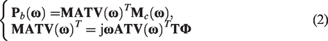
Train-induced vibration and structure-borne noise radiating from the bridge can be treated as a steady process during the train’s passage, and bridge noise can be calculated in the frequency domain.^26,27 An acoustic transfer vector (ATV)-based method can be used to predict bridge noise, as follows²⁸

P_{b} (ω)= A T V {(ω)}^{T} V_{b} (ω)

(1)

where

P_{b} (ω)

is the sound pressure spectra emitted from the bridge;

A T V (ω)

is the transfer function between the sound pressure at selected field points and the surface velocity with a unit normal velocity applied on the element surface;

V_{b} (ω)

is the surface velocity vector;

T

is the matrix transpose operation and

ω

is the angular frequency vector.

The ATVs can be easily obtained using BEM, and the SPLs of the structure can be directly measured. The unknown surface velocities can then be reconstructed through inverse analysis. However, the number of structure surface elements is significantly larger than the number of measurement points.²² Thus, to permit accurate reconstruction, a large number of field points should be selected²⁸ for the measurement. The criteria for the number, location and density of measurement points can be found in Martinus et al.²⁹

MATV-based method

To improve the efficiency of the ATV-based method, an inverse method based on MATVs is presented in this study. MATVs are the transfer functions between the sound pressure at selected field points and modal displacements. The bridge noise can be expressed as³⁰

{\begin{cases} P_{b} (ω)= M A T V {(ω)}^{T} M_{c} (ω), \\ M A T V {(ω)}^{T} = j ω A T V {(ω)}^{T} T Φ \end{cases}

(2)

where

j = \sqrt{- 1}

;

M_{c} (ω)

is the modal coordinate spectra of the structure;

Φ

is the mode shape and

T

is the overall transfer matrix projecting the mode shape displacements in the outward normal direction of the structure surface.

The modal coordinate spectra $M_{c} (ω)$ can be calculated from the dynamic analysis of train-track-bridge when using the forward prediction method.¹³ In contrast, $M_{c} (ω)$ can be directly recovered from inverse analysis, provided the MATVs and measured SPLs are obtained, with no need to develop a train–track–bridge interaction model. Note that the number of structure surface elements (unknown surface velocities $V_{b} (ω)$ in equation (1)) is much larger than the mode numbers (unknown $M_{c} (ω)$ ) used in equation (2), especially for bridges with large surface areas. For instance, for the U-shaped concrete bridge used in Li et al.,² the number of mode shapes needed for forward prediction was only 111, while the acoustic model contained 7692 boundary elements. Thus, many more measurement points should be selected for the ATV-based inverse method than the MATV-based inverse method.

Generally, the measurement points are less than the unknown modal coordinate spectra; rather, the number of rows of $M A T V {(ω)}^{T}$ is less than the number of columns. Thus, the inverse procedure is an underdetermined problem. Regularisation techniques can be used to solve this ill-posed problem. Both QR factorisation with column pivoting³¹ and SVD with Tikhonov regularisation^32,33 were used in this study.

QR factorisation with column pivoting

QR factorisation with column pivoting is useful when $M A T V^{T}$ (m-by-n matrix) is rank deficient, which is given by³¹

M A T V^{T} = Q R S^{T}

(3)

where

Q

is an

m \times m

unitary matrix;

R

is an

m \times n

upper triangular matrix; m and n are the number of measurement points and mode shapes, respectively and

S

is a permutation matrix in which the diagonal elements in

R

are sorted in non-increasing order:

| r_{11} | \geq | r_{22} | \geq \dots \geq | r_{m m} |

The problem is referred to as finding a minimum norm solution of the modal coordinate spectra at each frequency. The minimum norm solution of $M_{c}$ can be obtained as follows³¹

M_{c} = S (\begin{array}{l} R_{11}^{- 1} C_{1} \\ 0 \end{array})

(4)

where

_{R}^{11}

is the submatrix in the first k rows and columns of

R

; k is the rank of

M A T V^{T}

and

C_{1}

contains the first k elements of

C

, where

C = Q^{T} P_{b}

SVD with Tikhonov regularisation

SVD is another tool commonly used to solve ill-posed problems. $M A T V^{T}$ can be written in the SVD form²⁰

M A T V^{T} = U \sum V^{*}

(5)

where

U

is an

m \times m

unitary matrix, which can be written as

U = (u_{1} \dots u_{m})

;

\sum

is a diagonal

m \times n

matrix with n non-negative singular values

(σ_{1} \dots σ_{n})

;

V

is an

n \times n

unitary matrix,

V = (v_{1} \dots v_{n})

and

*

is the complex transpose operation.

When measurement errors occur in $P_{b} (ω)$ in equation (2), the solution of $M_{c}$ can be unstable with a huge norm if all SVD components are used in the inverse analysis.²⁰ To suppress the influence of errors and single out a stable solution, additional constraints are needed. The well-known Tikhonov regularisation is used here to seek a solution $M_{c}$ as the minimiser of the weighted combination of the residual norm $‖ M A T V^{T} M_{c} - P_{b} ‖$ and the introduced side constraint $‖ L M_{c} ‖$ . Thus, the inverse problem can be written as a minimisation problem using Tikhonov regularisation³³

\min_{M_{c}} {_{‖ M A T V^{T} M_{c} - P_{b} ‖}^{2} + λ^{2}_{‖ L M_{c} ‖}^{2}}

(6)

where

λ

is the regularisation parameter, which can be obtained through the L-curve method;^20,33

‖ � ‖

is the Euclidean norm and

L

is the Tikhonov matrix, for which an identity matrix is used in this study (

L = I

Finally, the standard Tikhonov regularised solution can be written as

M_{c} = \sum_{i = 1}^{n} f_{i} \frac{u_{i}^{*} P_{b}}{σ_{i}} v_{i}

(7)

where

f_{i} = \frac{σ_{i}^{2}}{(σ_{i}^{2} + λ^{2})}

is the Wiener filter.

The whole process of the inverse BEM used in this study is shown in Figure 1. Note that the reconstructed sound field should be compared with the measurement to validate the accuracy of the inverse model.

Figure 1.

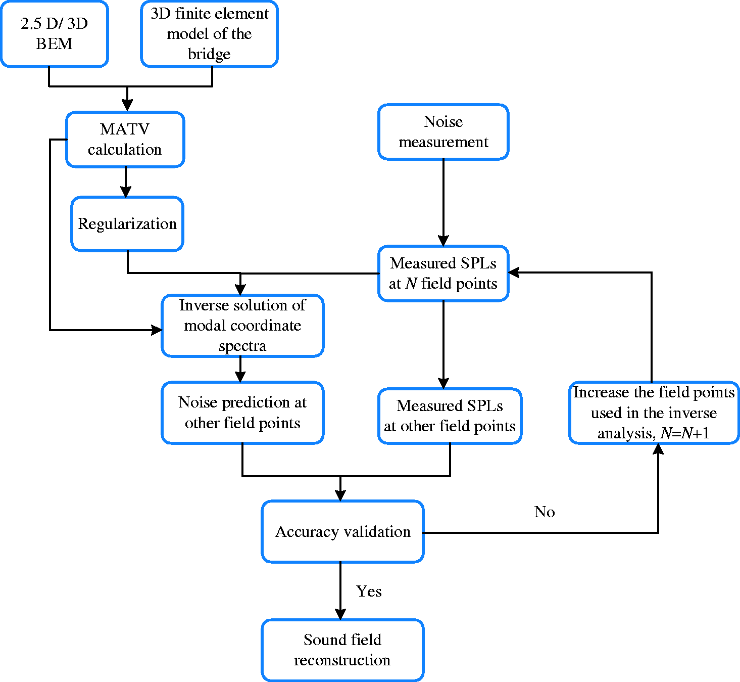
Flow diagram of the inverse BEM procedure.

Numerical and experimental validation

A box girder concrete bridge

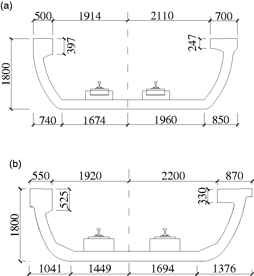
A three-span simple box girder concrete bridge with the standard span length of 30 m (Fig. 2) was selected to investigate the accuracy of the proposed inverse method. First, the train–track–bridge dynamic model and 2.5D BEM-based acoustic model¹³ were used to predict the sound pressure emitted from the box girder bridge. 3D finite elements and multiple rigid bodies were chosen to model the bridge and vehicles, respectively. The stiffness of the rail fastener in the horizontal and vertical directions used in this study was 20 and 60 MN/m, respectively. The damping of the fastener in the horizontal and vertical directions was set at 60 and 80 kN s/m, respectively. The four-axle trains comprised seven vehicles, with detailed model parameters listed in Li et al.² The rail roughness was generated in accordance with the rail limit roughness spectrum given in the ISO 3095 standard³⁴ in the space domain by using a trigonometric series method.² The MATVs of the bridge were calculated using the 2.5D BEM.¹³ The acoustic field point mesh is shown in Figure 3, with a total width of 30 m and height of 15 m.

Figure 2.

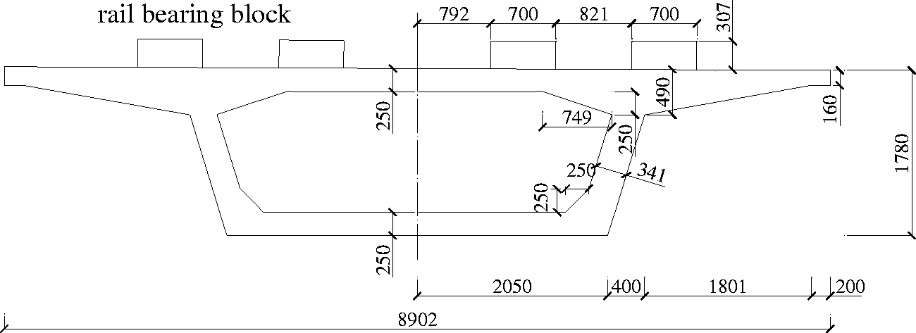
Geometry of the box girder bridge (unit: mm).

Figure 3.

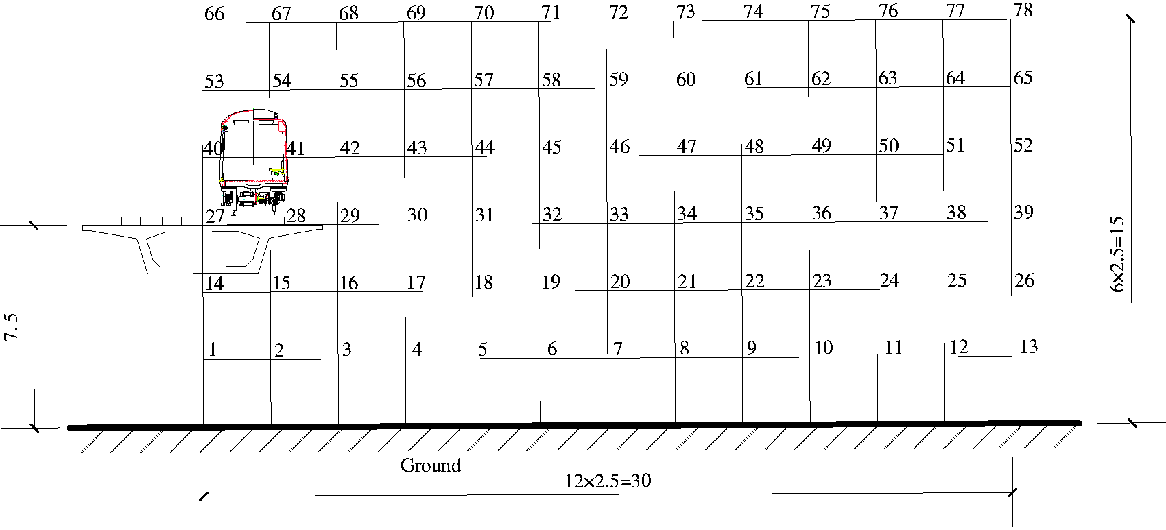
Field point mesh of the box girder bridge (unit: m).

A small number of field points were then selected and treated as virtual measurement points, and the sound pressure spectra $P_{b} (ω)$ of these points obtained from the forward numerical procedure were used to perform an inverse analysis. Both QR factorisation with column pivoting and SVD with Tikhonov regularisation were used. Reproduction of the remaining sound field points was then performed. Table 1 shows the five cases of virtual measurement points used in the inverse analysis. Cases B-1 and B-2 contain four field points in two rows and one column, respectively. Case B-3 contains five field points in one row. Cases B-4 and B-5 contain 10 and 14 field points in multiple rows, respectively. A comparison of the SPLs calculated using the inverse method and forward prediction with the first three cases are shown in Figure 4, which shows that the reconstructed SPLs using QR factorisation agree well with the forward prediction, while SVD with Tikhonov regularisation generally underestimates the SPLs for the first three cases of virtual measurement points. Figure 5 shows the reconstructed results obtained using the virtual measurement points of cases B-4 and B-5. It can be seen that SVD with Tikhonov regularisation can achieve greater accuracy with an increase in virtual measurement points, while the precision of the QR decomposition method is less dependent on the number of virtual measurement points, provided that more than four field points are selected. To further verify the precision of the proposed inverse method, Figures 6 and 7 present the contour maps of the difference between the SPLs computed using forward prediction and inverse analysis with different virtual measurement points. For the structure used in this study, inverse BEM with QR factorisation is more efficient than SVD with Tikhonov regularisation. After much trial and error, it was found that four to five virtual measurement points (cases B-1 to B-3) permitted an accurate reconstruction of the noise radiating from the box girder bridge while using the QR factorisation method, with an error of less than 3.5 dB. However, for the structures used in this study, many more field points (14 field points for case B-5) are needed to accurately reconstruct the sound field when using SVD with Tikhonov regularisation. For other cases with fewer virtual measurement points (cases B-1 to B-4), the SVD with Tikhonov regularisation method significantly underestimates bridge noise, and the error decreases with the increase of virtual measurement points used in the inverse analysis.

Figure 4.

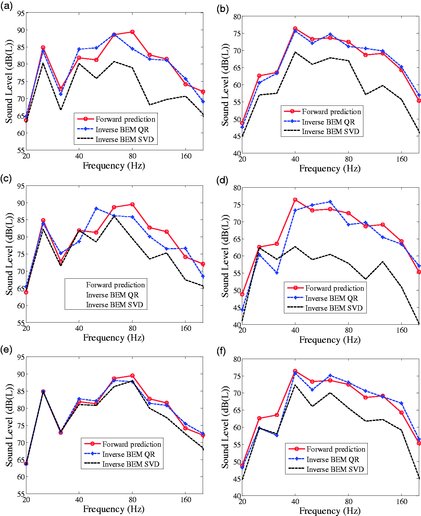
SPLs at different field points: (a) field point 28, case B-1; (b) field point 78, case B-1; (c) field point 28, case B-2; (d) field point 78, case B-2; (e) field point 28, case B-3 and (f) field point 78, case B-3.

Figure 5.

SPLs at different field points: (a) field point 28, case B-4; (b) field point 78, case B-4; (c) field point 28, case B-5 and (d) field point 78, case B-5.

Figure 6.

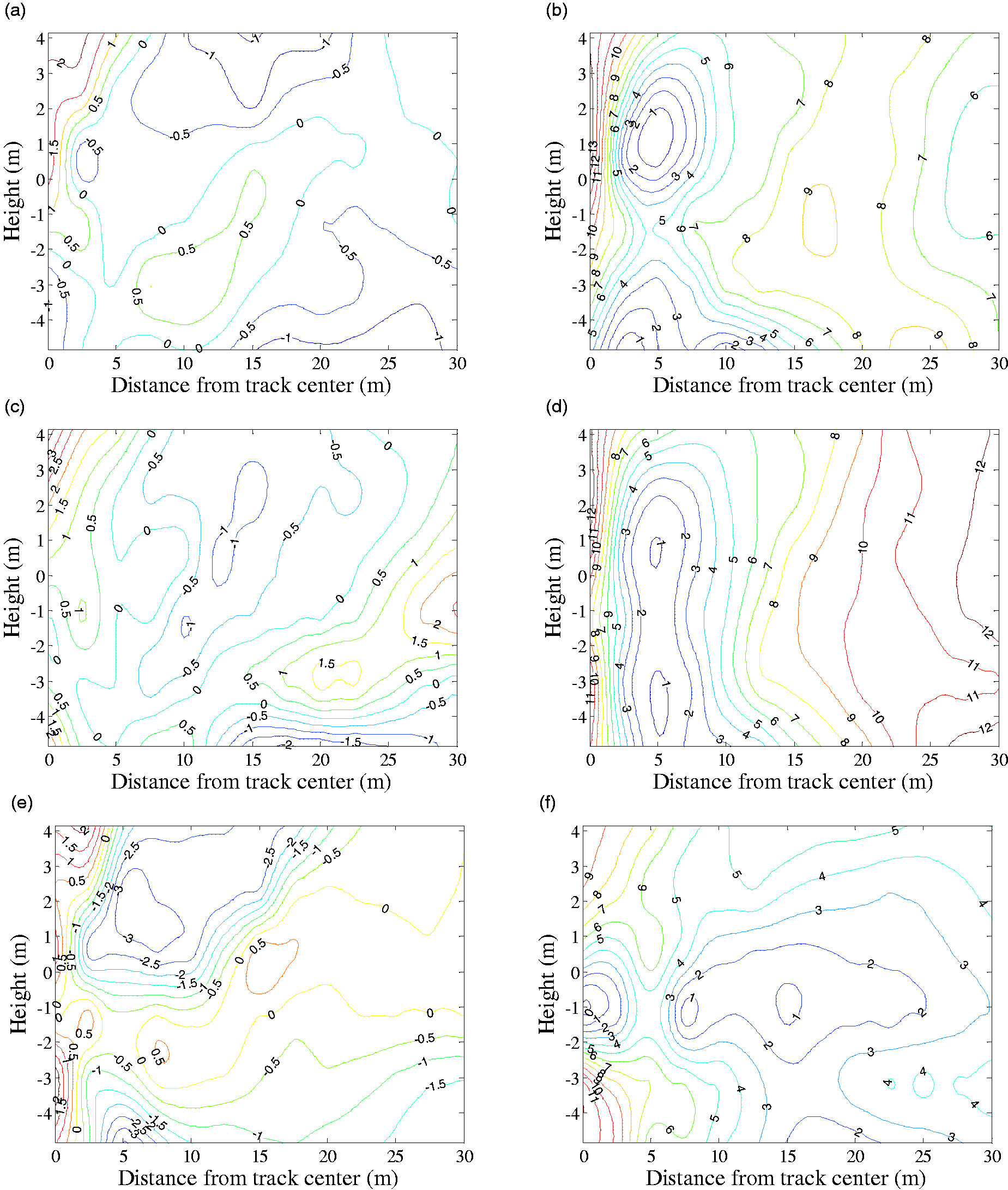
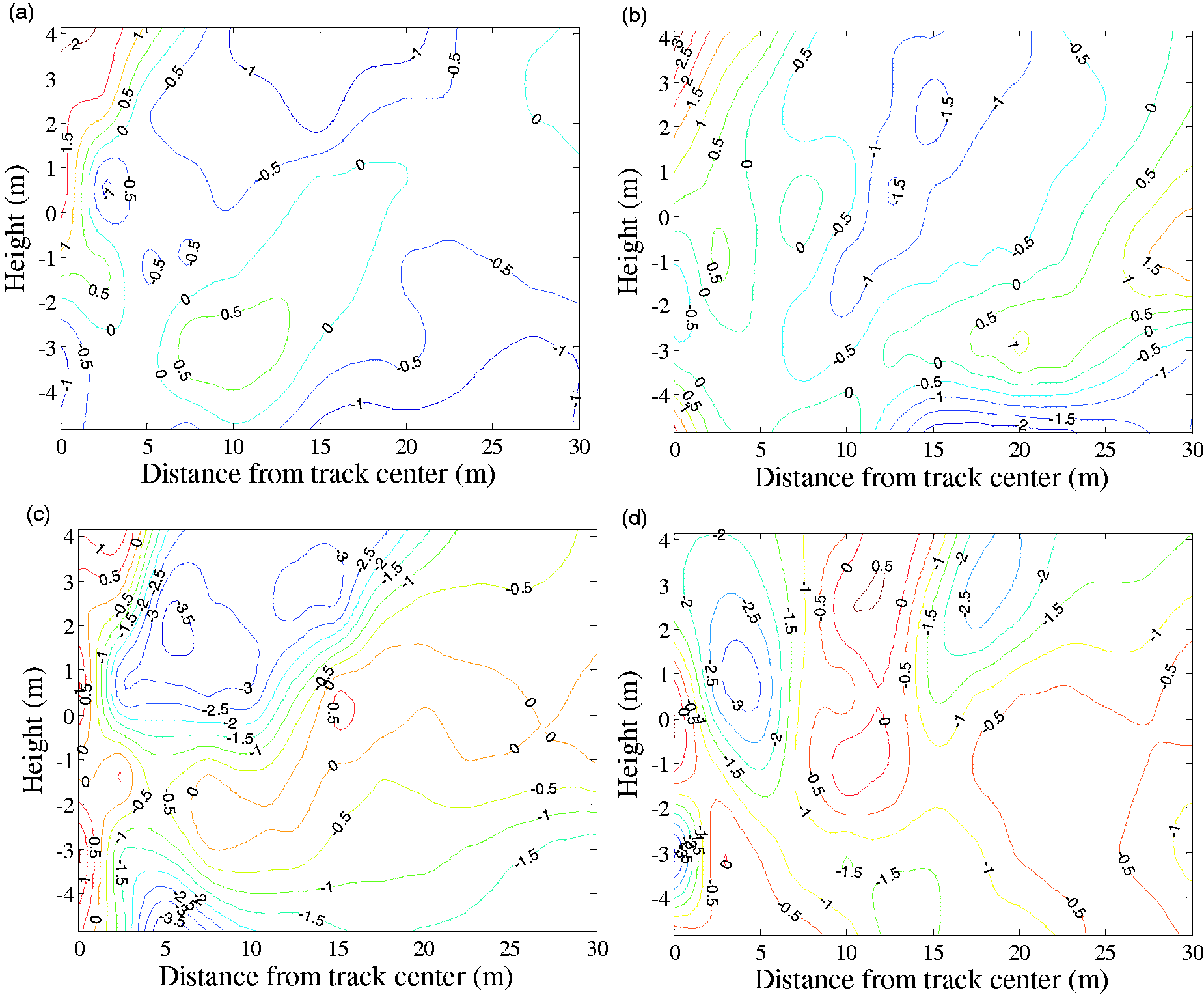
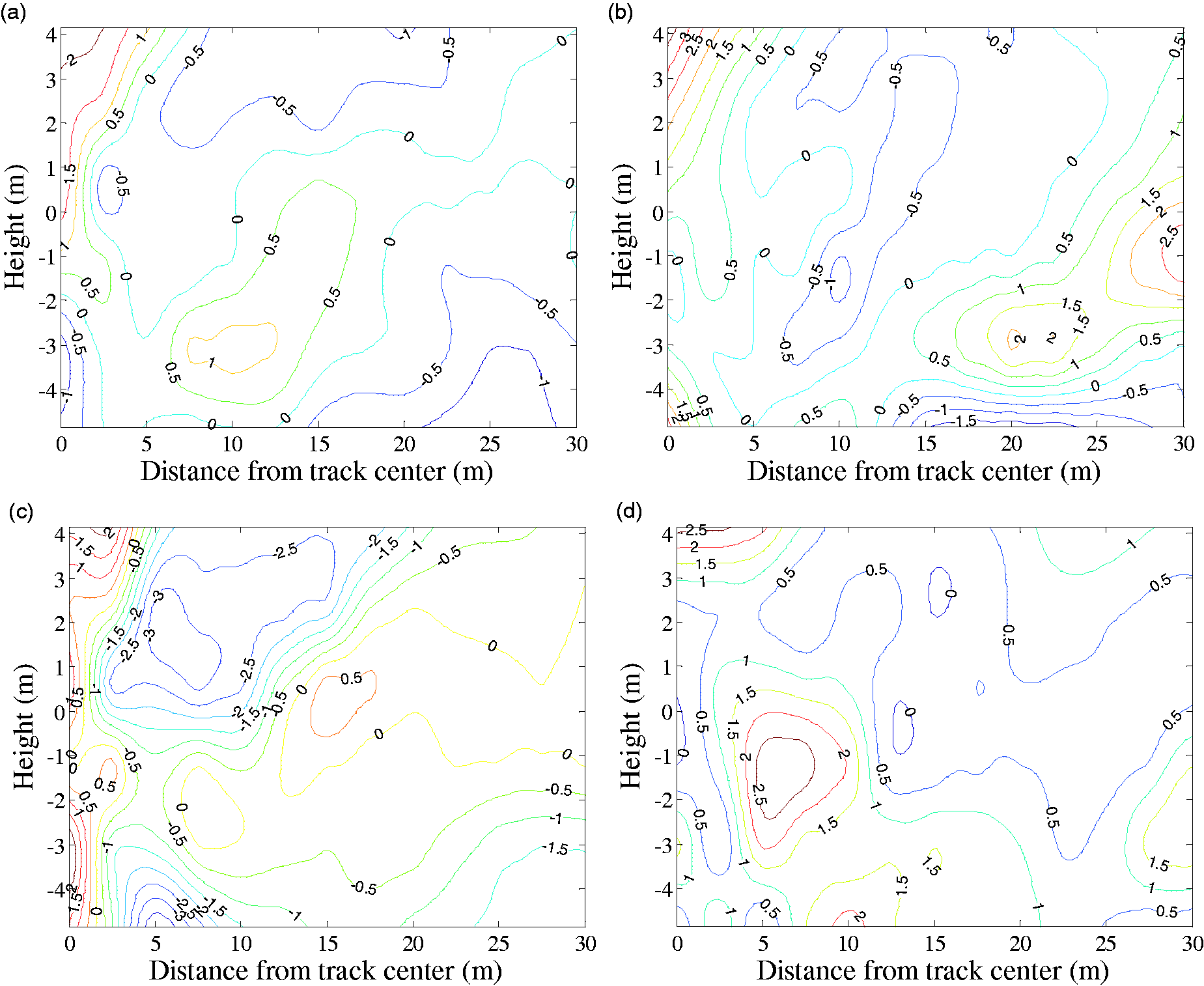
Contour maps of the difference between the forward prediction and the inverse BEM (unit: dB): (a) QR, case B-1; (b) SVD, case B-1; (c) QR, case B-2; (d) SVD, case B-2; (e) QR, case B-3 and (f) SVD, case B-3.

Figure 7.

Contour maps of the difference between the forward prediction and the inverse BEM (unit: dB): (a) QR, case B-4; (b) SVD, case B-4; (c) QR, case B-5 and (d) SVD, case B-5.

Table 1.

Cases of pseudo-measurement positions for the box girder bridge.

Case	Field point number
B-1	2, 5, 42 and 52
B-2	3, 16, 29 and 42
B-3	27, 30, 33, 36 and 39
B-4	1, 3, 12, 15, 23, 27, 32, 37, 45, and 52
B-5	1, 3, 12, 15, 23, 27, 32, 37, 40, 45, 52, 56, 60, and 72

To study the stability of the inverse method, 5 and 15% white Gaussian noise was added to the sound pressure data at the virtual measurement points listed in Table 1. The sound field was then reconstructed. Figures 8 and 9 show the recovered solutions with different cases using QR factorisation and SVD with Tikhonov regularisation, respectively. The added white Gaussian noise has insignificant influence on the reconstructed SPLs at most frequency bands, and only a slightly larger error occurs at some frequency bands with the additional increase of noise. Comparison between Figures 8 and 9 shows that many more field points are needed to lead to good reconstruction while using SVD with Tikhonov regularisation in the presence of Gaussian noise. Furthermore, the QR factorisation method is more sensitive to the added noise, while the SVD method is more stable in the presence of data noise. Figures 10 and 11 give contour maps of the difference between the accurate forward prediction and the reconstructed results with 15% noise using the two methods. Figure 10 shows that reasonably good reconstruction can be achieved in the whole space when using the QR factorisation method, even with 15% white Gaussian noise (maximum error less than 3.5 dB). Figure 11 shows that when sufficient field points are used, the SVD method can also lead to good results in the presence of 15% white Gaussian noise (maximum error less than 2.5 dB).

Figure 8.

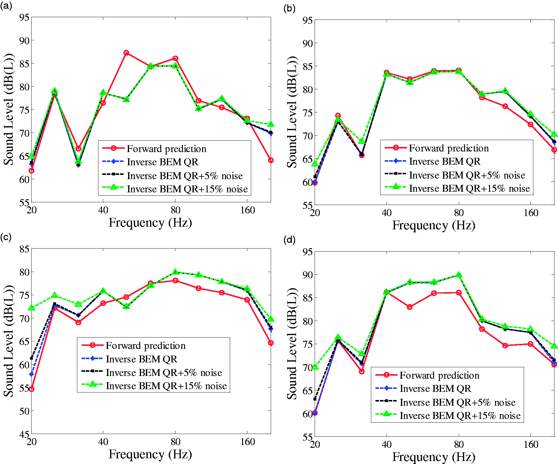
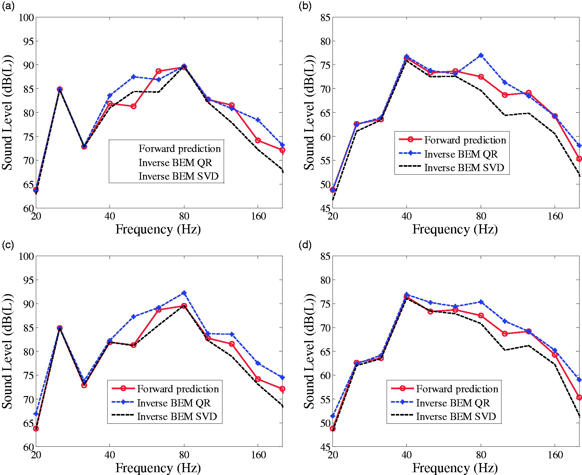
SPLs at different field points (QR): (a) field point 67, case B-1; (b) field point 55, case B-2; (c) field point 5, case B-3 and (d) field point 42, case B-4.

Figure 9.

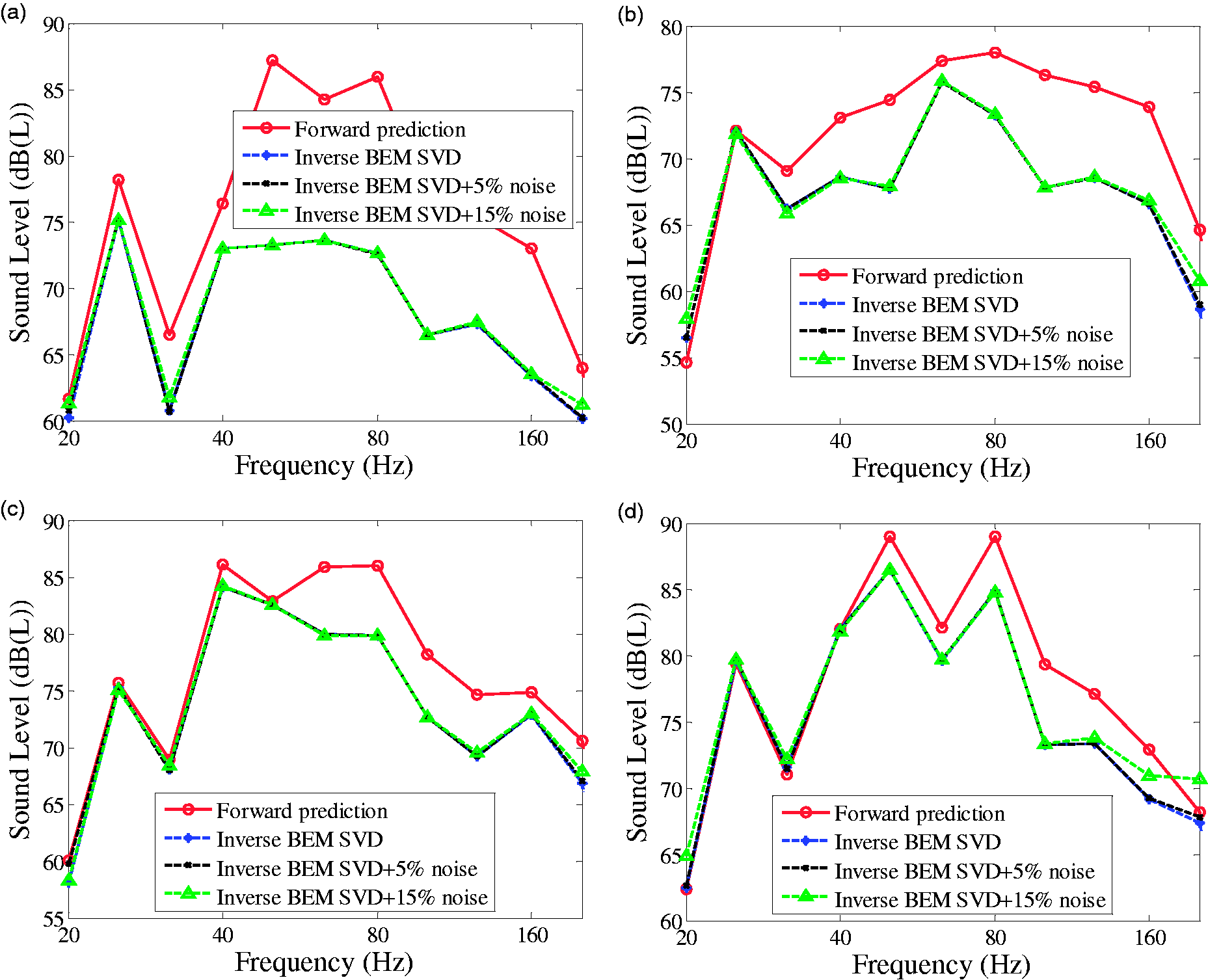
SPLs at different field points (SVD): (a) field point 67, case B-1; (b) field point 5, case B-3; (c) field point 42, case B-4 and (d) field point 66, case B-54.

Figure 10.

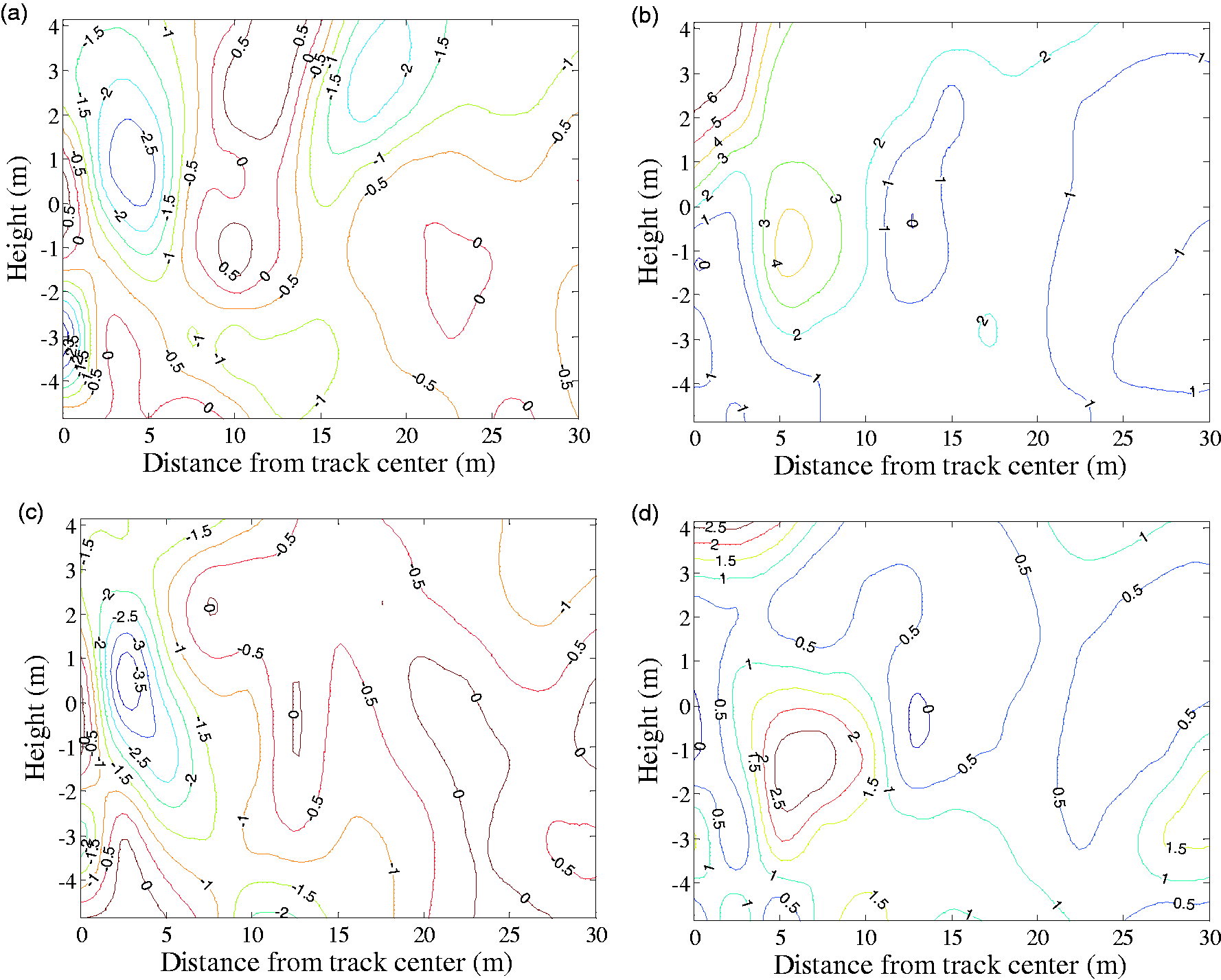
Contour maps of the difference between the forward prediction and the inverse BEM with 15% noise (unit: dB): (a) QR, case B-1; (b) QR, case B-2; (c) QR, case B-3 and (d) QR, case B-4.

Figure 11.

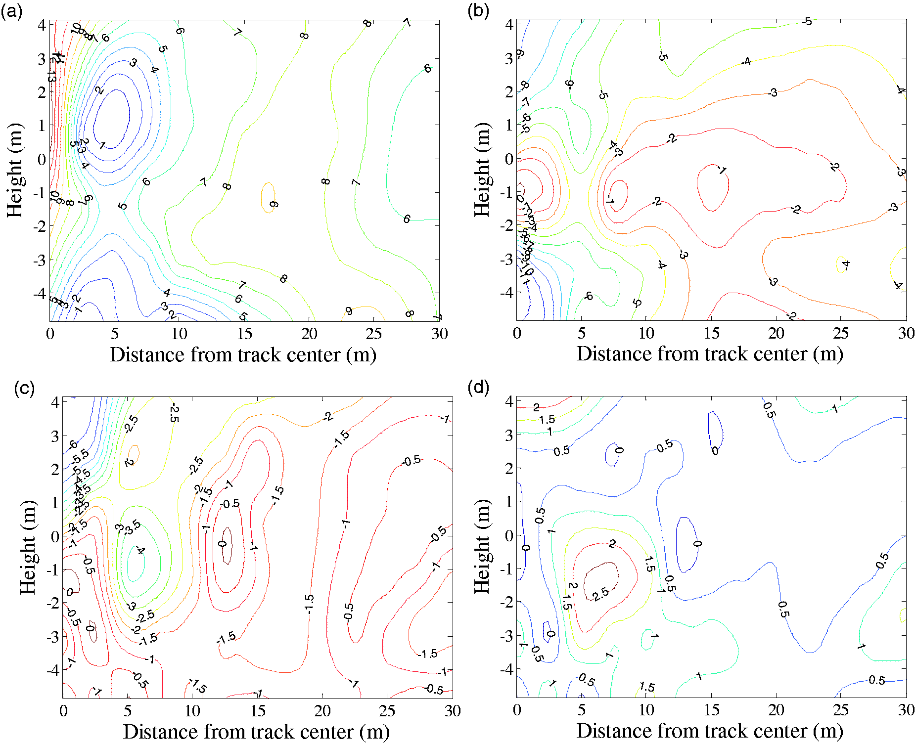
Contour maps of the difference between the forward prediction and the inverse BEM with 15% noise (unit: dB): (a) SVD, case B-1; (b) SVD, case B-3; (c) SVD, case B-4 and (d) SVD, case B-5.

Note that the mode shapes of the finite element model are usually different from those of the real bridge. Thus, the box girder bridge was varied by reducing the elastic modulus of the rail-bearing blocks by 5% to simulate local stiffness degradation and mode shape difference between the measurement and numerical model. The mode shapes of the varied model, which differed from the modes used in the forward prediction, were then used for noise reconstruction. The contour maps of the difference between the predicted and reconstructed results are shown in Figure 12. This reveals that good accuracy can be achieved even if a varied model is used for noise reconstruction. Thus, the proposed inverse BEM is a robust and reliable numerical method.

Figure 12.

Contour maps of the difference between the forward prediction and the inverse BEM with a varied structure (unit: dB): (a) QR, case B-1; (b) QR, case B-2; (c) QR, case B-3 and (d) SVD, case B-5.

Two U-shaped girder concrete bridges

A simple U-shaped concrete girder used in Shanghai metro line 8 (Figure 13(a)) and another U-shaped concrete girder used in Shanghai metro line 16 (Figure 13(b)) were chosen to further study the application and suitability of the inverse procedure. The standard span lengths of the two U-shaped girders are 25 and 30 m, respectively. Field tests were conducted to record the sound pressures radiating from the U-shaped girder induced by passing trains in lines 8 and 16, respectively. Five microphones in the same plane were installed beneath the U-shaped girder at the mid-span of line 8 (Figure 14). Six microphones were installed around the bridge of line 16 (three above the girder and three beneath), as shown in Figure 15. A 3D finite element model and 2.5D boundary element model were developed to obtain the MATVs of the U-shaped girders.¹³ The ground and structure surface were set to be rigid in the acoustic model. The QR factorisation method was used in the following study due to the limited number of measurement points.

Figure 13.

Cross sections of the U-shaped girder bridges (unit: mm): (a) line 8; (b) line 16.

Figure 14.

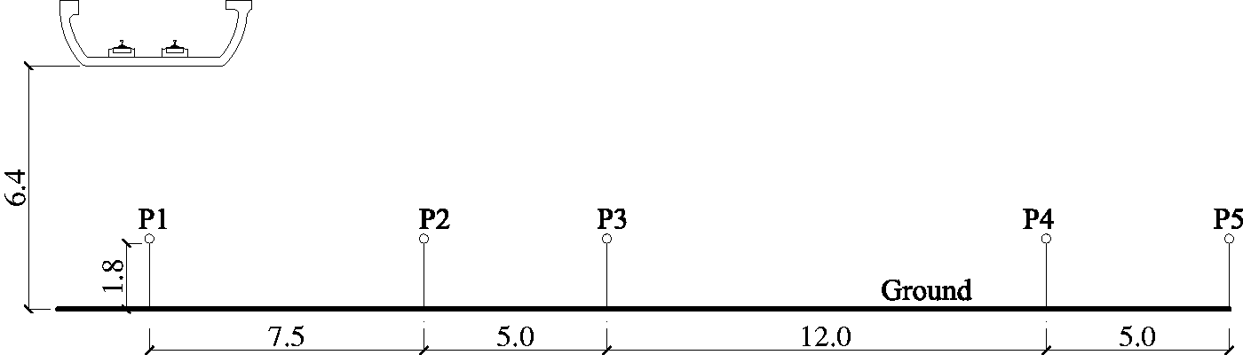
Layout of measurement positions of line 8 (unit: m).

Figure 15.

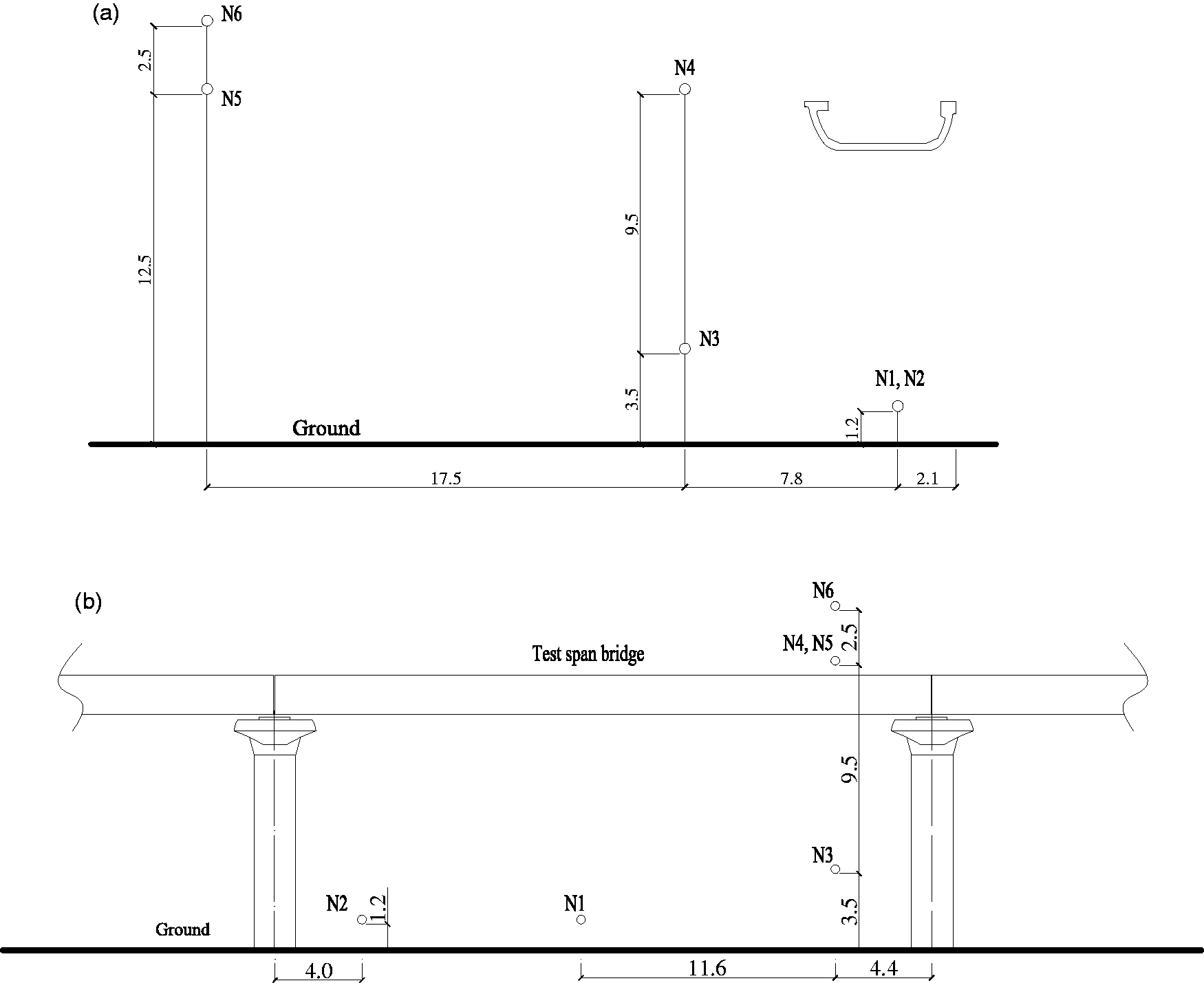
Layout of measurement positions of line 16 (unit: m): (a) section view; (b) elevation view.

The natural frequencies and mode shapes obtained from the finite element model differ from the results of the measurements. Thus, the finite element model should be updated in accordance with the measurements. However, the high-order mode shapes are usually local vibrations, which are difficult to directly identify from measurement. For the field tests conducted in this study, a very limited number of accelerometers were used to record bridge vibrations. Thus, only the first vertical and lateral natural frequencies were identified from measurement. The first-order lateral and vertical natural frequencies of the bridge (line 8) identified were 2.235 and 4.249 Hz, respectively. The finite element model was then tuned by modifying the elasticity modulus and mass of the bridge. The first lateral and vertical natural frequencies of the updated finite element model were 2.238 and 4.360 Hz, respectively.

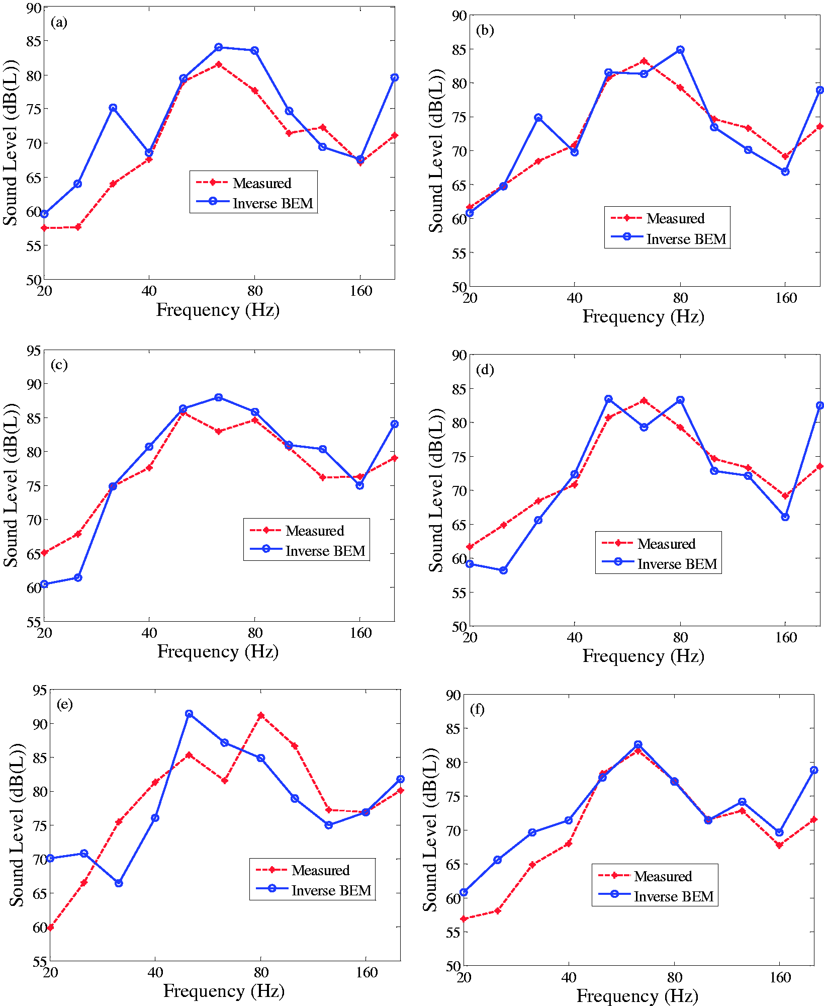
The measured results of four field points in line 8 were first used to reconstruct the acoustic field, and the results of the unused field point obtained using inverse analysis were then compared with the measurement. The cases of field points used in the inverse analysis for line 8 are listed in Table 2. Figures 16 and 17 compare the SPLs between the measurement and inverse BEM, with train speeds of 56 and 76 km/h, respectively. Generally, good agreement was found between the measurement and the reconstructed SPLs at most frequency bands with different train speeds.

Figure 16.

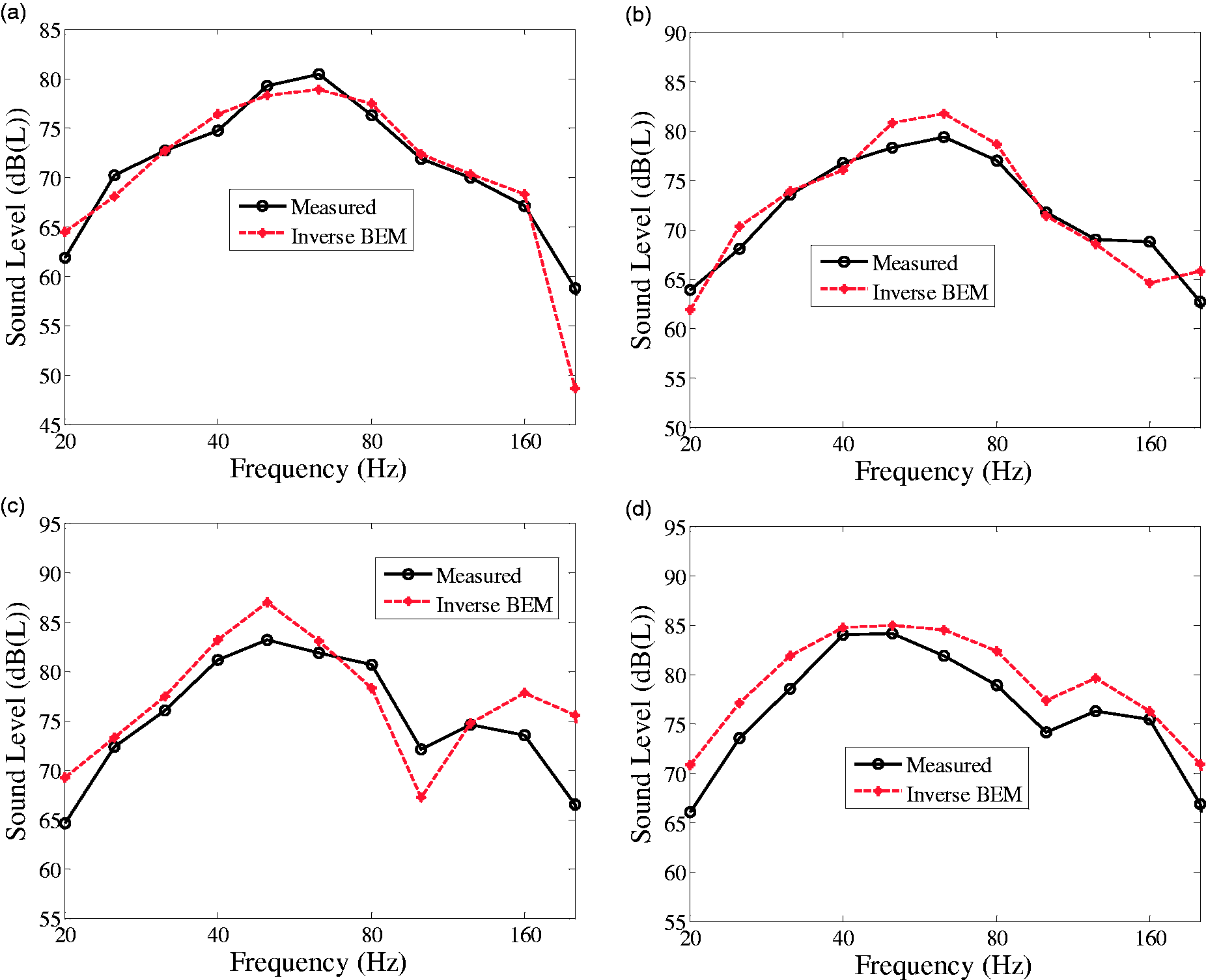
Comparison between measured and inverse BEM SPLs in line 8, train speed 56 km/h: (a) P5, case U8-1; (b) P4, case U8-2; (c) P3, case U8-3 and (d) P2, case U8-4.

Figure 17.

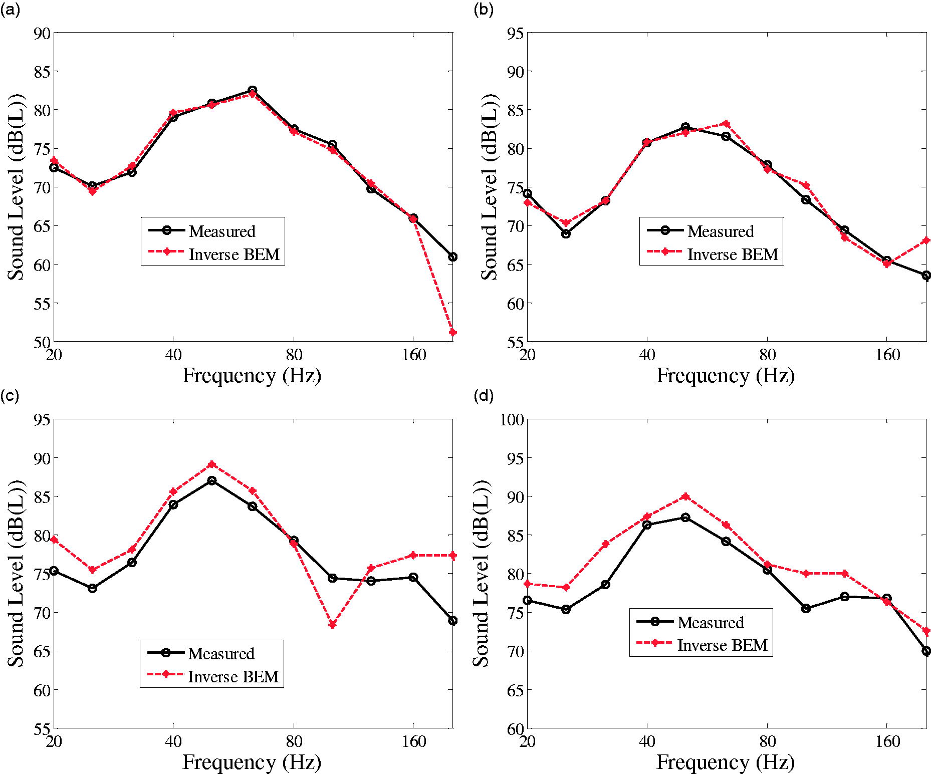
Comparison between measured and inverse BEM SPLs in line 8, train speed 76 km/h: (a) P5, case U8-1; (b) P4, case U8-2; (c) P3, case U8-3 and (d) P2, case U8-4.

Table 2.

Cases of the inverse analysis for the U-shaped girder bridge in line 8.

Case	Field points used for reconstruction
U8-1	P1, P2, P3 and P4
U8-2	P1, P2, P3 and P5
U8-3	P1, P2, P4 and P5
U8-4	P1, P3, P4 and P5

The SPLs of the U-shaped girder bridge in line 8 were simulated using forward prediction in our previous work.¹³ Song et al.¹³ showed that the SPLs obtained using forward prediction were smaller than the measured results, especially for the far field point (P5, about 3 dB error). Figure 18 shows the contour maps of the SPLs obtained using the inverse method proposed in this study and those obtained from forward prediction as presented in Song et al.¹³ The sound pressure distribution of the two pictures is similar. The reconstructed SPLs are slightly larger than the forward prediction, which agrees better with the measurements.

Figure 18.

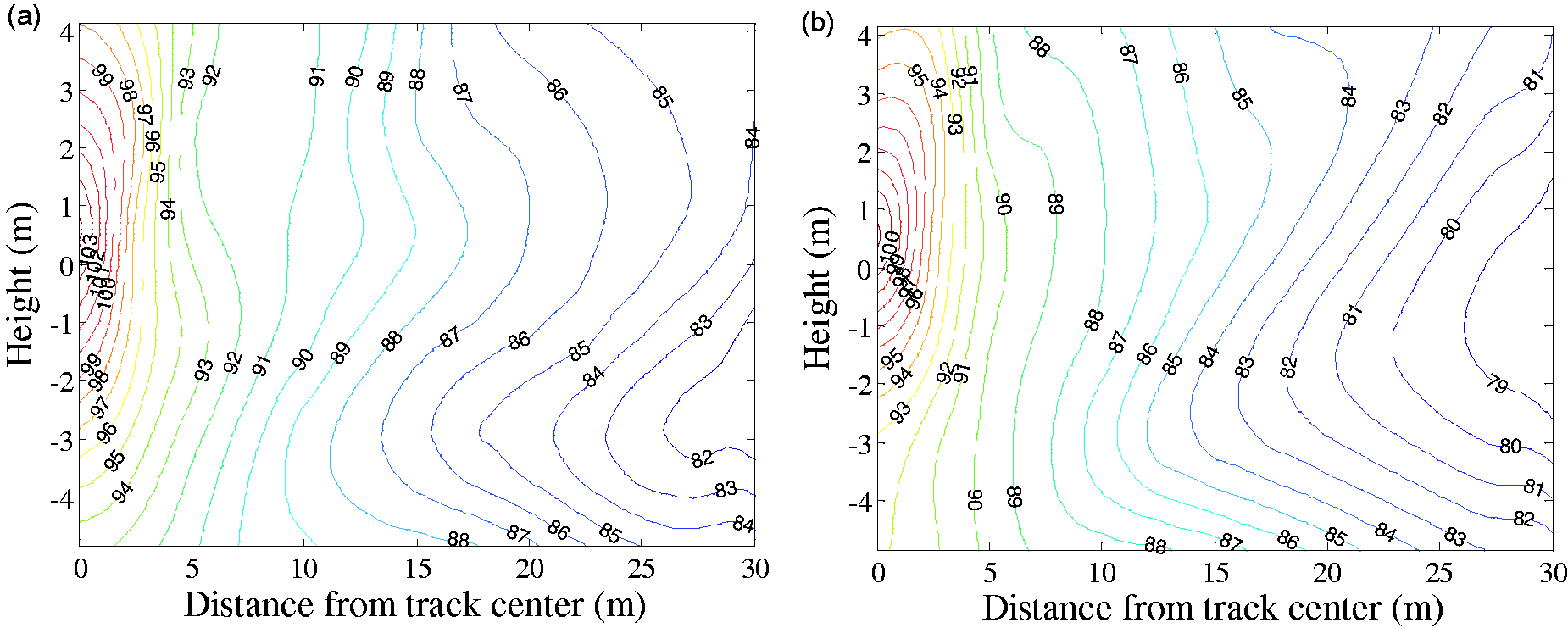
Contour maps of the U-shaped girder bridge in line 8 (unit: dB): (a) inverse method, U8-1; (b) numerical method.¹³

The measured data of four field points in line 16 were also used to reconstruct the corresponding acoustic field, and the results of the remaining two field points were used for validation. Table 3 lists the three cases used in the inverse analysis. Figures 19 and 20 show the SPLs of the remaining two field points in each case obtained from measurement and inverse analysis, with train speeds of 80 and 100 km/h, respectively. It can be seen from the comparison that the reconstructed results agree well with the measured SPLs, provided that no fewer than four field points are used in inverse analysis.

Figure 19.

Comparison between measured and inverse BEM SPLs in line 16, train speed 80 km/h: (a) N5, case U16-1; (b) N6, case U16-1; (c) N4, case U16-2; (d) N6, case U16-2; (e) N3, case U16-3 and (f) N5, case U16-3.

Figure 20.

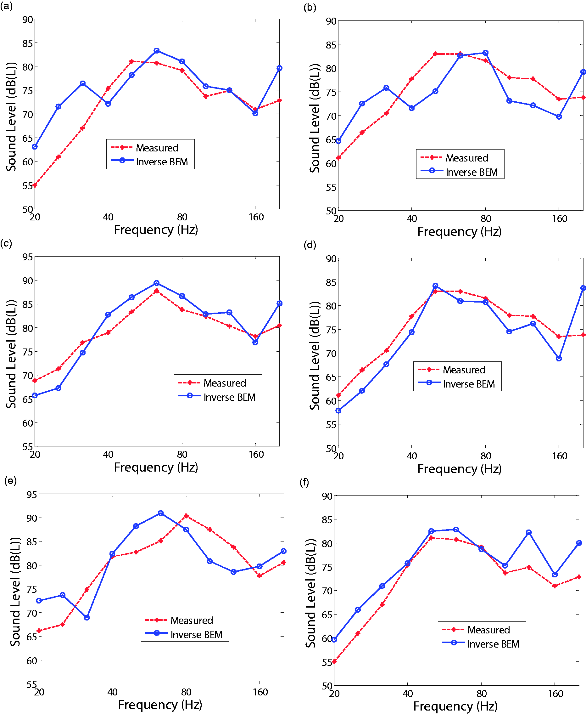
Comparison between measured and inverse BEM SPLs in line 16, train speed 100 km/h: (a) N5, case U16-1; (b) N6, case U16-1; (c) N4, case U16-2; (d) N6, case U16-2; (e) N3, case U16-3 and (f) N5, case U16-3.

Table 3.

Cases of the inverse analysis for the U-shaped girder bridge in line 16.

Case	Field points used for reconstruction
U16-1	N1, N2, N3 and N4
U16-2	N1, N2, N3 and N5
U16-3	N1, N2, N4 and N6

Conclusions

An inverse procedure was presented to reconstruct the acoustic field radiating from bridges by combining the MATVs and the SPLs at a small number of measurement points. First, the sound radiation of a concrete box girder bridge was calculated using a forward prediction method, and the associated numerical results were utilised to validate the accuracy and robustness of the inverse procedure. Field tests of two U-shaped girders were then used for further validation. Three major conclusions can be drawn from this study:

MATV-based inverse analysis needs only a small number of measurement points to enable an accurate reconstruction of the acoustic field radiating from bridges, which reduces the requirement for test equipment.

To perform accurate inverse analysis for the simple bridges used in this study, SVD with Tikhonov regularisation needs many more measurement points than QR factorisation with column pivoting.

Reasonably good reconstruction of the bridge noise can be achieved when four to five field points are used in the inverse analysis with the QR-factorisation method. The inverse method is reliable and robust even with 15% white Gaussian noise added to the sound pressure data.

More field measurements should be conducted to further verify the accuracy and adaptability of the proposed procedure.

Footnotes

Declaration of conflicting interests

The author(s) declared no potential conflicts of interest with respect to the research, authorship, and/or publication of this article.

Funding

The author(s) disclosed receipt of the following financial support for the research, authorship and/or publication of this article: The study was supported by the National Natural Science Foundation of China (No. 51608116), and the Natural Science Foundation of Jiangsu (No. BK20160681).

References

Stiebel

Lölgen

Gerbig

Innovative measures for reducing noise radiation from steel railway bridges. In: Proceedings of the 11th international workshop on railway noise, Uddevalla, Sweden, 9–13 September 2013, pp.173–180. Berlin, Heidelberg: Springer.

DJ.

Concrete bridge-borne low-frequency noise simulation based on vehicle-track-bridge dynamic interaction. J Sound Vib 2012; 331: 2457–2470.

Pawlaczyk-Luszczynska

Dudarewicz

Waszkowska

et al . Annoyance related to low frequency noise in subjective assessment of workers. J Low Freq Noise Vib Active Control 2009; 28: 1–17.

Colaço

Alves Costa

Amado-Mendes

et al . Prediction of vibrations and reradiated noise due to railway traffic: a comprehensive hybrid model based on a finite element method and method of fundamental solutions approach. J Vib Acoust 2017; 139: 061009–061010.

Mortensen

Poulsen

Annoyance of low frequency noise and traffic noise. J Low Freq Noise Vib Active Control 2000; 20: 193–196.

et al . A combined power flow and infinite element approach to the simulation of medium-frequency noise radiated from bridges and rails. J Sound Vib 2016; 365: 134–156.

Thompson

DJ.

Prediction of rail and bridge noise arising from concrete railway viaducts by using a multilayer rail fastener model and a wavenumber domain method. Proc IMechE Part F: J Rail Rapid Transit 2017; 232: 1326–1346.

Zhang

Wang

et al . Vibrational and acoustical performance of concrete box-section bridges subjected to train wheel–rail excitation: field tests and numerical analysis. Noise Control Eng J 2016; 64: 217–229.

Lee

Kim

Jang

WS.

Analysis of sound radiation from the coupling effect of vibrating noise and moving-vehicle noise on bridges. Can J Civil Eng 2005; 32: 881–898.

10.

Oostdijk

Weekenstroo

Vercammen

Noise prediction of a steel-concrete railway bridge using a FEM. In: Euronise 2015, Maastricht, the Netherlands, 31 May–3 June 2015, pp.2053–2058. Maastricht: Euronoise.

11.

Zhang

et al . A hybrid model for the prediction of low-frequency noise emanating from a concrete box-girder railway bridge. Proc IMechE Part F: J Rail Rapid Transit 2016; 230: 1242–1256.

12.

Zhang

Hao

et al . A case study of interior low-frequency noise from box-shaped bridge girders induced by running trains: its mechanism, prediction and countermeasures. J Sound Vib 2016; 367: 129–144.

13.

Song

et al . Structure-borne low-frequency noise from multi-span bridges: a prediction method and spatial distribution. J Sound Vib 2016; 367: 114–128.

14.

Sheng

Jones

CJC

Thompson

DJ.

Ground vibration generated by a harmonic load moving in a circular tunnel in a layered ground. J Low Freq Noise Vib Active Control 2003; 22: 83–96.

15.

Alves Costa

Calçada

Cardoso

AS.

Influence of train dynamic modelling strategy on the prediction of track–ground vibrations induced by railway traffic. Proc IMechE Part F: J Rail Rapid Transit 2012; 226: 434–450.

16.

Ngai

Lee

YY.

The control of structure-borne noise from a viaduct using floating honeycomb panel. JSME Int J Ser C 2006; 49: 494–504.

17.

Zhang

et al . Experimental research on noise emanating from concrete box-girder bridges on intercity railway lines. Proc IMechE Part F: J Rail Rapid Transit 2015; 229: 125–135.

18.

Weber

Kletschkowski

Sachau

Noise source identification in a 2D cavity based on inverse finite element method. J Low Freq Noise Vib Active Control 2010; 29: 147–159.

19.

Chappell

Harris

PJ.

A Burton–Miller inverse boundary element method for near-field acoustic holography. J Acoust Soc Am 2009; 126: 149–157.

20.

Schuhmacher

Hald

Rasmussen

et al . Sound source reconstruction using inverse boundary element calculations. J Acoust Soc Am 2003; 113: 114–127.

21.

Kletschkowski

Weber

Sachau

Identification of noise sources in an aircraft fuselage using an inverse method based on a finite element model. Acta Acust United Acust 2011; 97: 974–983.

22.

Herrin

Liu

Martinus

et al . Prediction of sound pressure in the far field using the inverse boundary element method. Noise Control Eng J 2010; 58: 74–82.

23.

Djamaa

Ouelaa

Pezerat

et al . Sound source localization by an inverse method using the measured dynamic response of a cylinder. Appl Acoust 2015; 88: 22–29.

24.

Zhang

et al . An inverse direct time domain boundary element method for the reconstruction of transient acoustic field. J Vib Acoust 2017; 139: 021013–021018.

25.

Song

DJ.

Investigation of rail noise and bridge noise using a combined 3D dynamic model and 2.5D acoustic model. Appl Acoust 2016; 109: 5–17.

26.

Luo

et al . Experimental study on ground vibration attenuation induced by heavy freight wagons on a railway viaduct. J Low Freq Noise Vib Active Control 2018; 37: 1–15.

27.

Liu

Pei

et al . Structure-borne noise of railway composite bridge: numerical simulation and experimental validation. J Sound Vib 2015; 353: 378–394.

28.

Tournour

Cremers

Guisset

Inverse numerical acoustics based on acoustic transfer vectors. In: 7th international congress on sound and vibration, Garmisch-Partenkirchen, Germany, 4–7 July 2000, pp.2069–2076.

29.

Martinus

Herrin

Seybert

AF.

Selecting measurement locations to minimize reconstruction error using the inverse boundary element method. J Comp Acoust 2007; 15: 531–555.

30.

Citarella

Federico

Cicatiello

Modal acoustic transfer vector approach in a FEM-BEM vibro-acoustic analysis. Eng Anal Bound Elem 2007; 31: 248–258.

31.

Anderson

Bai

Dongarra

Generalized QR factorization and its applications. Linear Algebra Appl 1992; 162–164: 243–271.

32.

Calvetti

Morigi

Reichel

et al . Tikhonov regularization and the L-curve for large discrete ill-posed problems. J Comput Appl Math 2000; 123: 423–446.

33.

Rozier

Lesselier

Inversion of a cylindrical vibrating body in shallow water from aspect-limited data using filtered SVD and the L-curve. Acta Acust United Acust 1996; 82: 717–728.

34.

ISO3095:2013. Railway applications-acoustics-measurement of noise emitted by railbound vehicles. Geneva, Switzerland: International Organization for Standardization, 2013.

Reconstruction of low-frequency bridge noise using an inverse modal acoustic transfer vector method

Abstract

Keywords

Introduction

Inverse BEM procedure

Acoustic transfer vector-based method

MATV-based method

QR factorisation with column pivoting

SVD with Tikhonov regularisation

Numerical and experimental validation

A box girder concrete bridge

Two U-shaped girder concrete bridges

Conclusions

Footnotes

Declaration of conflicting interests

Funding

References