
Abstract
In He’s frequency–amplitude formulation, the relationship between frequency and amplitude of a nonlinear oscillator can be obtained through residuals of two trial solutions. Although a high accurate solution can be obtained, this method has some space to be further improved. Here, we show that the calculation of the residuals can be further simplified without loss of accuracy. Duffing oscillator with high nonlinearity is used as an example to show the solution process and accuracy.
Introduction
Nonlinear problems play an important role not only in all areas of physics but also in many other disciplines, such as electronics, chemistry, biomechanics, physiology, textile engineering, and nanotechnology, because fundamental principles of most phenomena in the world are essentially nonlinear. In general, it is very difficult to solve nonlinear problems accurately. After decades of continuous efforts, some excellent methods appeared in open literature, such as the homotopy perturbation methods,1–11 the variational iteration method,12–17 the parameter expansion method, 18 the max–min approach, 19 the variational approach,20–23 the Hamiltonian approach, 24 the energy balance method, 25 the stability analysis,26–29 and the simple formulae for fast prediction of frequency. 30
To solve nonlinear oscillators, Chinese mathematician Prof. Ji-Huan He proposed a simple but effect frequency–amplitude formulation.31–34 He’s frequency–amplitude formulation was used by many authors with great success.35–39 In this study, we will suggest an alternative form of the residuals for He’s frequency–amplitude formulation and apply it to high-order Duffing oscillator.
He’s frequency–amplitude formulation
To illustrate the basic idea of He’s frequency–amplitude formulation,3,31–34 we first consider an algebraic equation in the form

Letting x1 and x2 be two trial solution of equation (1), we obtain two remainders f (x1) and f (x2), respectively. According to an ancient Chinese method, its approximate solution can be expressed

This formula generally gives us an accurate solution, though the calculation procedure is very easy.
Now we consider a generalized nonlinear oscillator with initial conditions in the following form


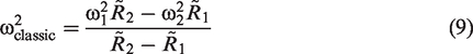
According to classic procedure of He’s frequency–amplitude formulation, the frequency of the nonlinear oscillator equation (3) can be computed approximately by
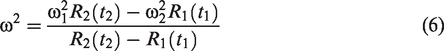
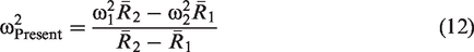
From these equations, the approximate frequency of equation (3) can also be calculated
Modification of He’s frequency–amplitude formulation
In He’s frequency–amplitude formulation equation (9), the function effects on residuals given in equations (7) and (8) are neglected when the phases
Equation (9) can be rewritten as
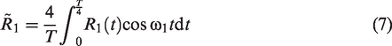
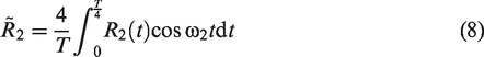
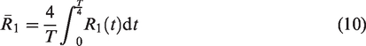
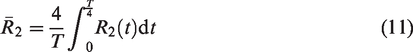
Actually, equations (10) and (11) are, respectively, geometric averages of the residuals of equations (4) and (5) in the internal
Example
To show the effectiveness of our modification, we consider a generalized Duffing oscillator in the form
40

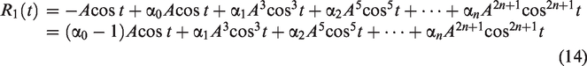
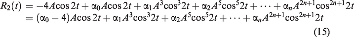
Choosing two trial functions
Classic process
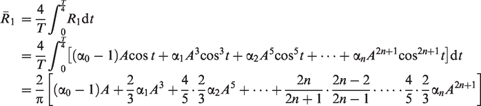
Substituting equations (14) and (15) into equations (7) and (8), respectively, the weighted residuals can be calculated
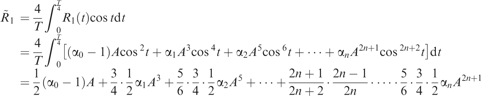
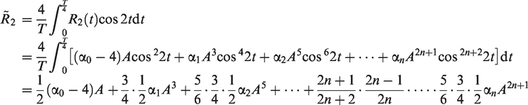
We get the frequency of the nonlinear oscillator, which is
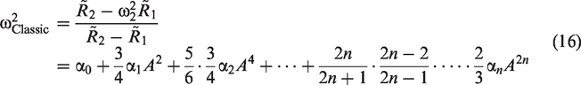
If
if n = 3

Present process
Now we substitute equations (14) and (15) into equations (10) and (11), respectively, the geometric average of the residuals can be expressed as
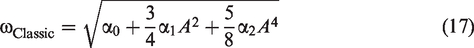
If n = 2, the frequency–amplitude relationship obtained as

if n = 3

Error analysis
For large values of α2 or α3, the relative errors of the approximate frequencies of equations (17), (18), (20), and (21) are, respectively, as follows


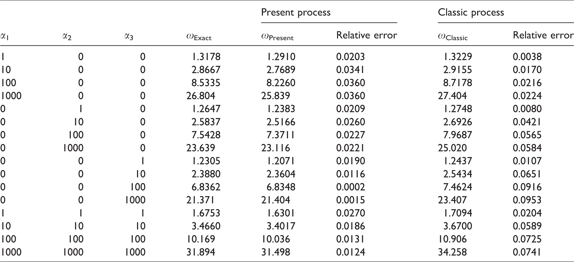
Comparison of the approximate frequencies (ωClassic and ωPresent) obtained by equations (18) and (21) with the exact frequencies ωExact is made in Table 1 for different values of α1, α2, and α3, where the exact frequencies ωExact are determined by equation (37) in the Appendix. All present solutions of ωPresent are in good agreement with the exact ones. Other comparisons between the approximate solutions and the exact ones can also be found in Figures 1 and 2, in which the present solution is overlapping with the exact one for A = α0 =1, α1 = α2 = 0, α3 = 100. From the table and the figures, we could see that the errors of the present solutions ωPresent are decreasing when the values of α2 and α3 increase.
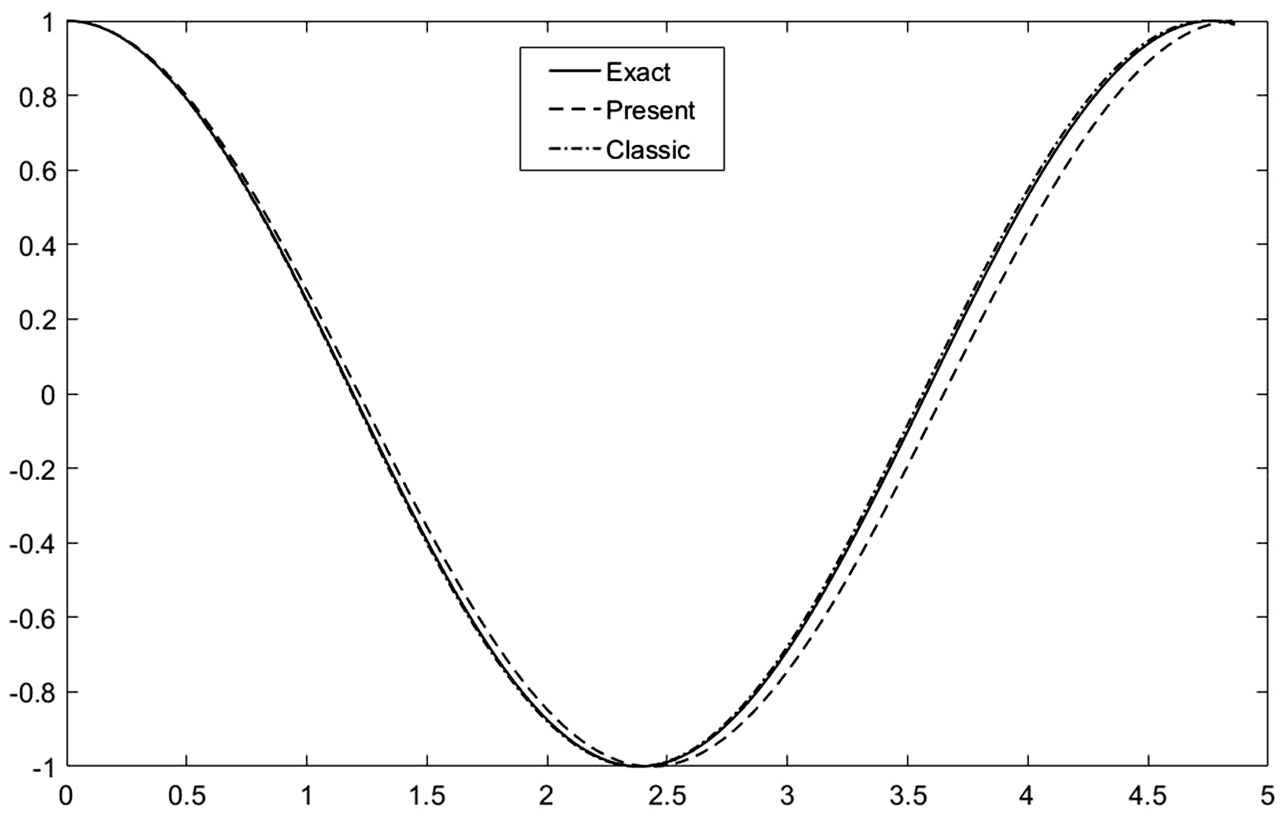
Comparison of present and classic solution with exact one for A = α0 = α1 =1, α2 = α3 = 0, the present solution gives an exact match with the exact one.
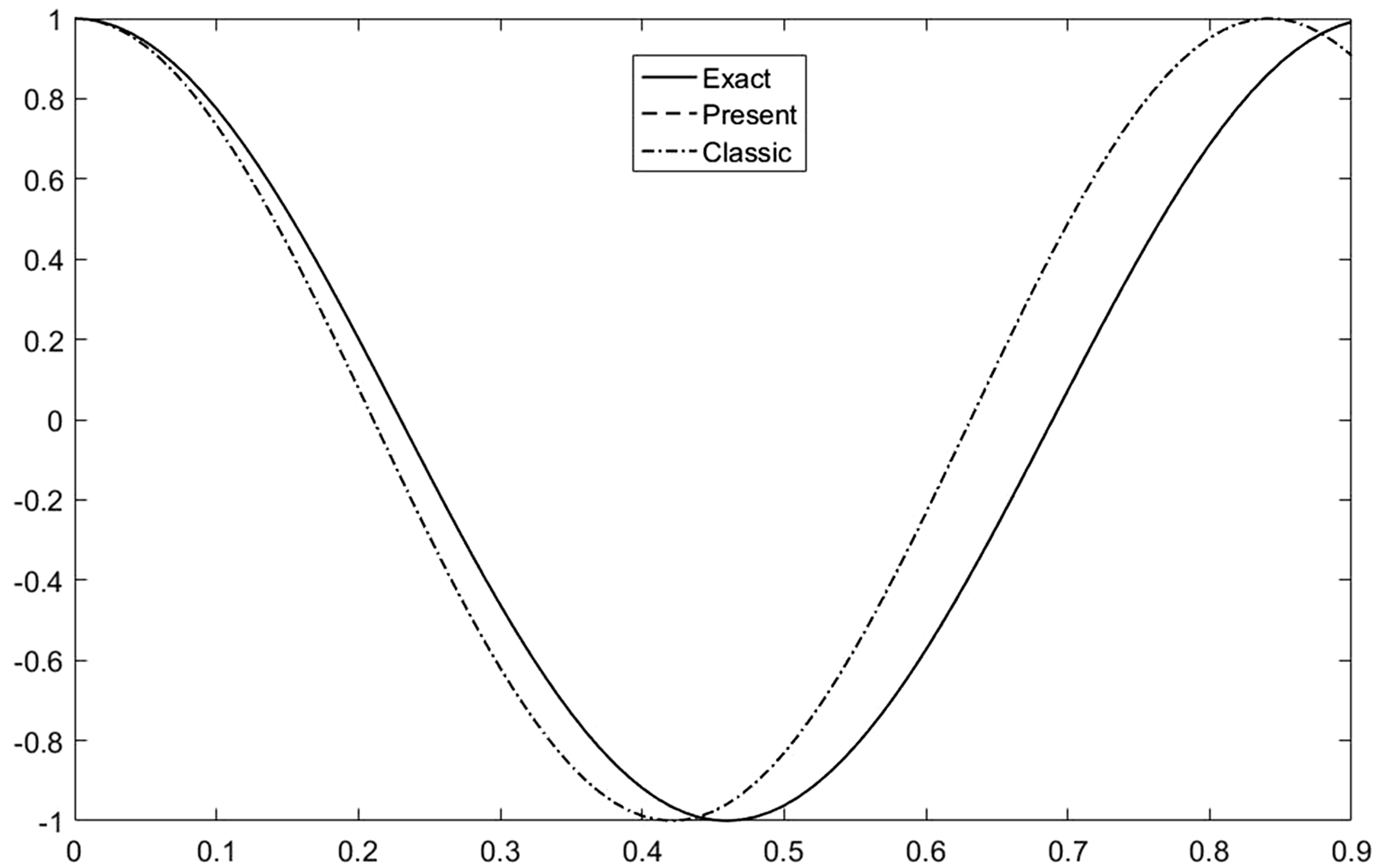
Comparison of present and classic solution with exact one for A = α0 =1, α1 = α2 = 0, α3 = 100, the present solution gives an exact match with the exact one.
Relative errors of solutions from present and classic process (A = α0 = 1).
Conclusion
He’s frequency–amplitude formulation modified with geometric averages of residuals can produce quite accurate solutions, especially for high-order Duffing oscillators.
Footnotes
Declaration of conflicting interests
The author(s) declared no potential conflicts of interest with respect to the research, authorship, and/or publication of this article.
Funding
The author(s) received no financial support for the research, authorship, and/or publication of this article.