Sage Journals: Discover world-class research

Abstract

In this paper an analysis of the nonlinear dynamic behavior and control of an atomic force microscope system is described. Phase plane trajectories, spectrum analysis, bifurcation analysis, the Poincare cross-section, the maximal Lyapunov exponent, and other numerical analysis methods were used to observe and verify the dynamic characteristics and the differential equations for the system. The results showed that at specific excitation frequencies, the system will exhibit nonlinear behavior that may be cyclic, multi-cyclic or acyclic. A Psim circuit simulation using the same parameters showed the same nonlinear behavior, as did laboratory circuit implementations. The results also showed than an understanding and control of the dynamic characteristics would not be an easy task. However, they could be used as a basis for the suppression and control of nonlinear behavior and vibration in atomic force microscope systems. A proportional-derivative system was also used, with particle swarm optimization, to find the control parameters K_p and K_D and a fuzzy controller was used to compare the results. The controller simulation and hardware implementation both effectively inhibited the nonlinear behavior and were most helpful for the control and enhancement of measurement accuracy.

Keywords

Atomic force microscope nonlinear behavior Psim circuit proportional-derivative system particle swarm optimization

Introduction

The atomic force microscope (AFM) is a kind of scanning probe microscope that can image almost any type of specimen surface, including polymers, ceramics, glass, and biological samples. It can operate in a vacuum, gas or liquid environment. Atomic force microscopy is used in many different fields, strength of materials, biotechnology,¹ micro-electro-mechanical systems, and many others. Scanning can be carried out in several different ways: contact mode, non-contact mode,² and tapping mode. The extensive use of AFM has resulted in a substantial amount of research. Many studies of cantilever action and the forces involved have been made and a theory has arisen with respect to nonlinear cantilever behavior.^3,4 Any nonlinear interaction between the probe tip and the sample surface can seriously affect the proper dynamic behavior of the cantilever.

In 1999, Aimé et al. investigated a nonlinear oscillation model with a single degree of freedom using perturbation to calculate the dynamic behavior of the micro-cantilever associated with the van der Waals force. Results showed that linear analysis cannot be used to explain the frequency drift phenomenon, nor why frequency drift becomes greater when there are small changes in the distance between the probe and the sample. The nonlinear behavior of an oscillation model allows observation of the relationship between resonant frequency drift and the distance between the probe and the sample.⁵ Ashhab et al. considered the van der Waals force⁶ and Lennard-Jones potential energy⁷ in a single degree of freedom oscillator model. They analyzed the dynamic behavior of the system using sinusoidal excitation and used the Melnikov method to predict the chaos which is likely to appear when the damping, excitation frequency, and balance of the system are within a certain range. Galerkin truncation is a relatively common method used in the study of nonlinear problems, and in 2003, Rützel et al. used first-order Galerkin truncation to study free cantilever and excitation vibration parameters in Lennard-Jones potential energy.⁸ Burnham et al.'s study^9,10 showed that the dynamic behavior of an AFM system micro-cantilever will become chaotic under certain specific conditions.

To enhance the measurement accuracy of the AFM, dynamic analysis was used to study the nonlinear behavior of the probe where chaotic phenomena appeared in the presence of nonlinear force. To counter the impact of irregular chaotic oscillation on measurement resolution, proportional-derivative (PD) and fuzzy control^11–13 were used for comparison and suppression. Particle swarm optimization (PSO)¹⁴ and the genetic algorithm (GA)^15,16 were used to search for the parameters K_p and K_D to be used for control and stabilization of the AFM operation. The inhibitory effect of the controllers was compared to increase the reliability of the algorithms and parameters. Psim circuit simulation was used to verify the nonlinear dynamic characteristics in a mathematical model of an AFM system and was also the basis for implementation of the model as an actual physical circuit. This study provides a thorough understanding of the nonlinear behavior of an AFM system using PD and fuzzy control for the inhibition of irregular system behavior.

Dynamic analysis

The theoretical analysis of AFM

This section describes the AFM differential equation (1) proposed by Rützel et al.⁸ When the Lennard-Jones potential formula is used to calculate the van der Waals force between the probe tip and the surface atoms of the sample, it is assumed that the Bernoulli-Euler beam theory is applicable, the impact of the axial force on the boom is negligible, and the cantilever and sample material is Si–Si (111)^17–19

\begin{array}{l} ρ A \ddot{u} (x, t) + E I (u^{''''} (x, t) + w^{*''''} (x)) \\ = (- \frac{A_{1} R}{180 {(Z - w * (L) - u (L, t) - Y \sin Ω t)}^{8}} + \frac{A_{1} R}{6 {(Z - w * (L) - u (L, t) - Y \sin Ω t)}^{2}}) \times δ (x - L) + ρ A Ω^{2} Y \sin Ω t \end{array}

(1)

Figure 1 shows several stages of deformation of the AFM cantilever and its relationship with the sample. Figure 1(a) shows the first state in the equation where the cantilever is stationary and in equilibrium. At this time the distance from the probe tip to the sample surface is Z, as shown in the figure. The second state, seen in Figure 1(b) illustrates the interaction of the applied force between the probe tip atoms and the sample surface atoms. 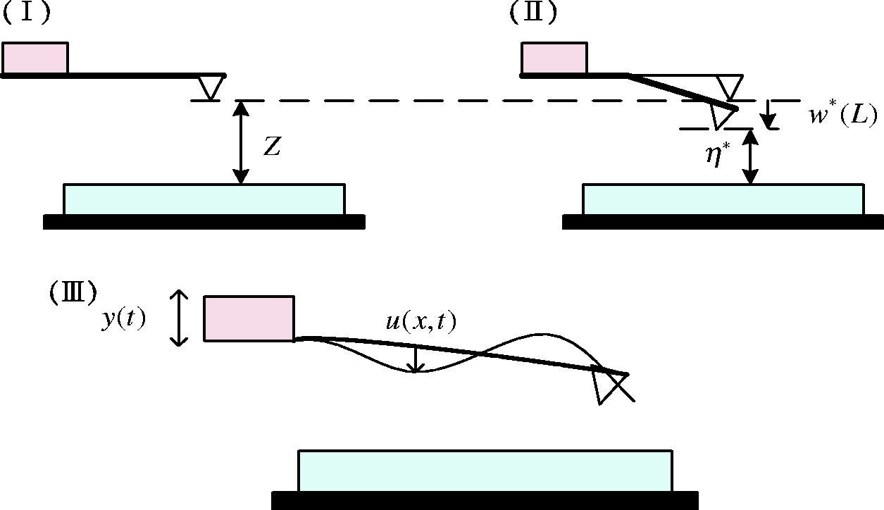Here the cantilever shows a deflection of $w^{*} (L)$ and the gap between the probe and sample at equilibrium is $η^{*} = Z - w^{*} (L)$ . In the last state, as shown in Figure 1(c), the cantilever has a deflection of $u (x, t)$ caused by piezoelectric element harmonic motion $y (t) = Y \sin Ω t$ .

Figure 1.

Atomic force microscope cantilever deformation in the tapping mode.

The equation (1) is made dimensionless and simplified,⁸ to give the dimensionless mathematical model shown below

{\dot{X}}_{1} = X_{2}

(2)

{\dot{X}}_{2} = - S_{1} X_{2} - X_{1} + S_{2} + \frac{S_{3}}{{(1 - X_{1} - S_{6} \sin (Ω τ))}^{8}} + \frac{S_{4}}{{(1 - X_{1} - S_{6} \sin (Ω τ))}^{2}} + S_{5} Ω^{2} S_{6} \sin (Ω τ)

(3)

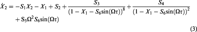
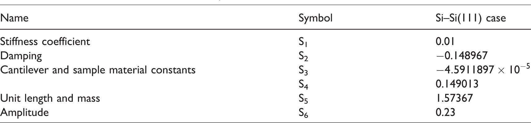
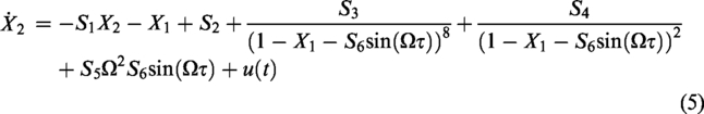
In these equations, X₁ represents the displacement of the probe tip. The fourth and fifth terms in equation (3) are van der Waals force calculated by the dimensionless Lennard-Jones potential formula. The last term is the cantilever harmonic motion, and Ω is the exciting frequency explored by dynamic analysis in this study, the other parameters are shown in Table 1.

Table 1.

Coefficients of the dimensionless equation.

Name	Symbol	Si–Si(111) case
Stiffness coefficient	S₁	0.01
Damping	S₂	−0.148967
Cantilever and sample material constants	S₃	$- 4 .5911897 \times 10^{- 5}$
Cantilever and sample material constants	S₄	0.149013
Unit length and mass	S₅	1.57367
Amplitude	S₆	0.23

Analysis of nonlinear behavior

Parameter definitions

This section focuses on the observation and exploration of nonlinear behavior generated by the system at excitation frequency Ω under different parameters. The relevant parameter values S₁∼S₆,¹⁰ are set as shown in Table 1, the dimensionless equations (2) and (3) are then used with Matlab/Simulink to simulate an AFM system. The differential equations are solved using the Runge-Kutta method. The solution involves the use of five kinds of numerical analysis to verify consistency of the dynamic behavior of the system.

Phase plane trajectories

Figure 2 shows traces of the phase plane trajectories when the probe displacement and speed are Ω = 0.46, 1.0, 2.0, and 3.0. The trajectories for Ω = 0.46, and 2.0, shown in Figure 2(a) and (c), are quite confusing and irregular and the dynamic behavior is clearly aperiodic. However, for Ω = 1.0 and 3.0, the trajectory is relatively stable and regular, as can be seen in Figure 2(b) and (d), and motion is periodic.

Figure 2.

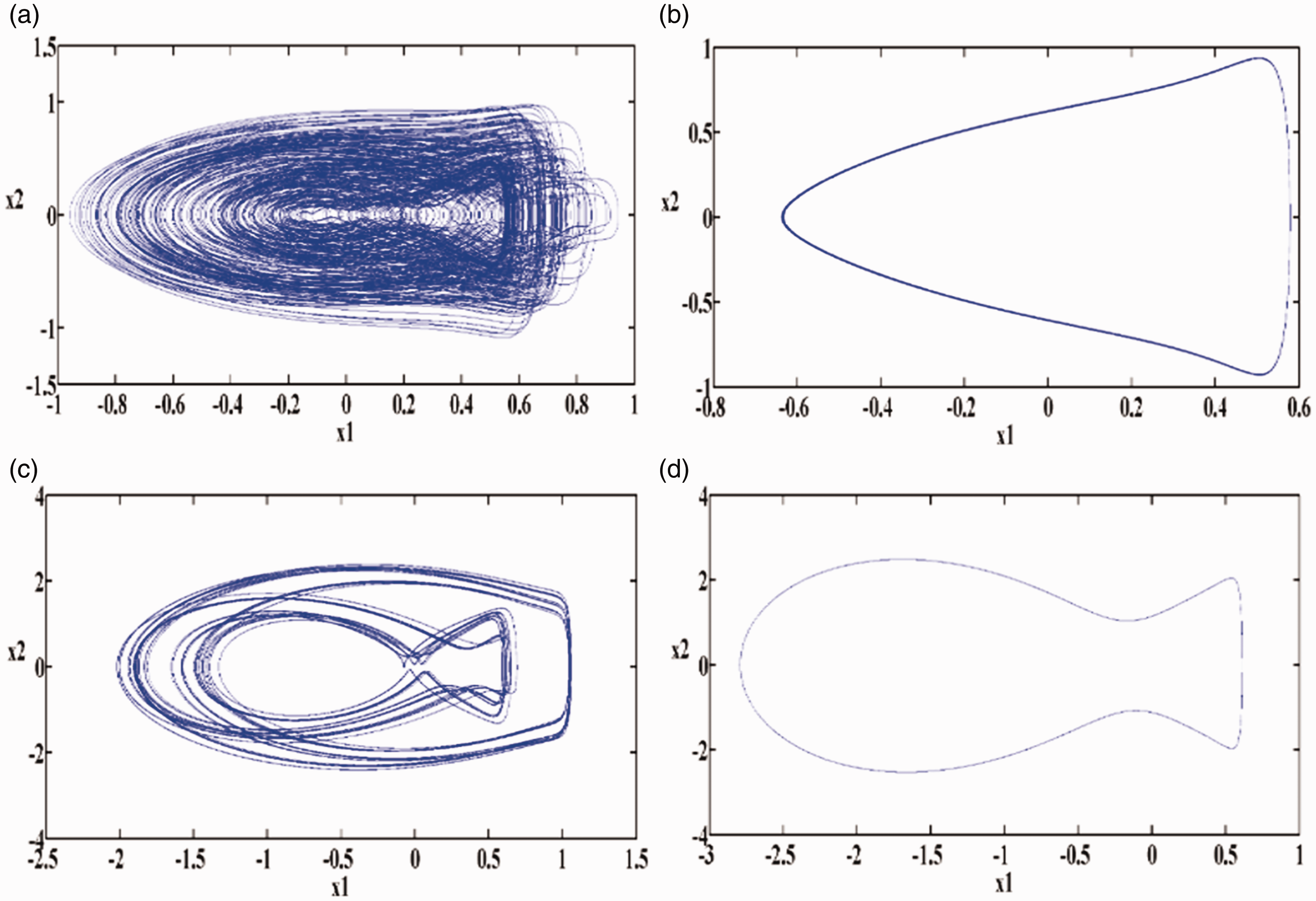
Phase plane trajectory patterns: (a) Ω = 0.46, (b) Ω = 1.0, (c) Ω = 2.0, and (d) Ω = 3.0.

Spectrum analysis

This section presents the findings from the spectrum analyses of probe displacement X₁ and speed signals X₂. For Ω = 1.0 and 3.0, the spectrum analysis trace shown in Figure 3(b) and (d) shows a velocity and displacement response in which the main frequency appears regularly. The apparent motion of the cycle and the normalized spectrum frequency for Ω = 1.0 has a period of 1T. The Ω = 3.0 spectrum has a period of 3T. For Ω = 0.46 and 2.0, the spectrum is distributed, continuous, and acyclical, as shown in Figure 3(a) and (c).

Figure 3.

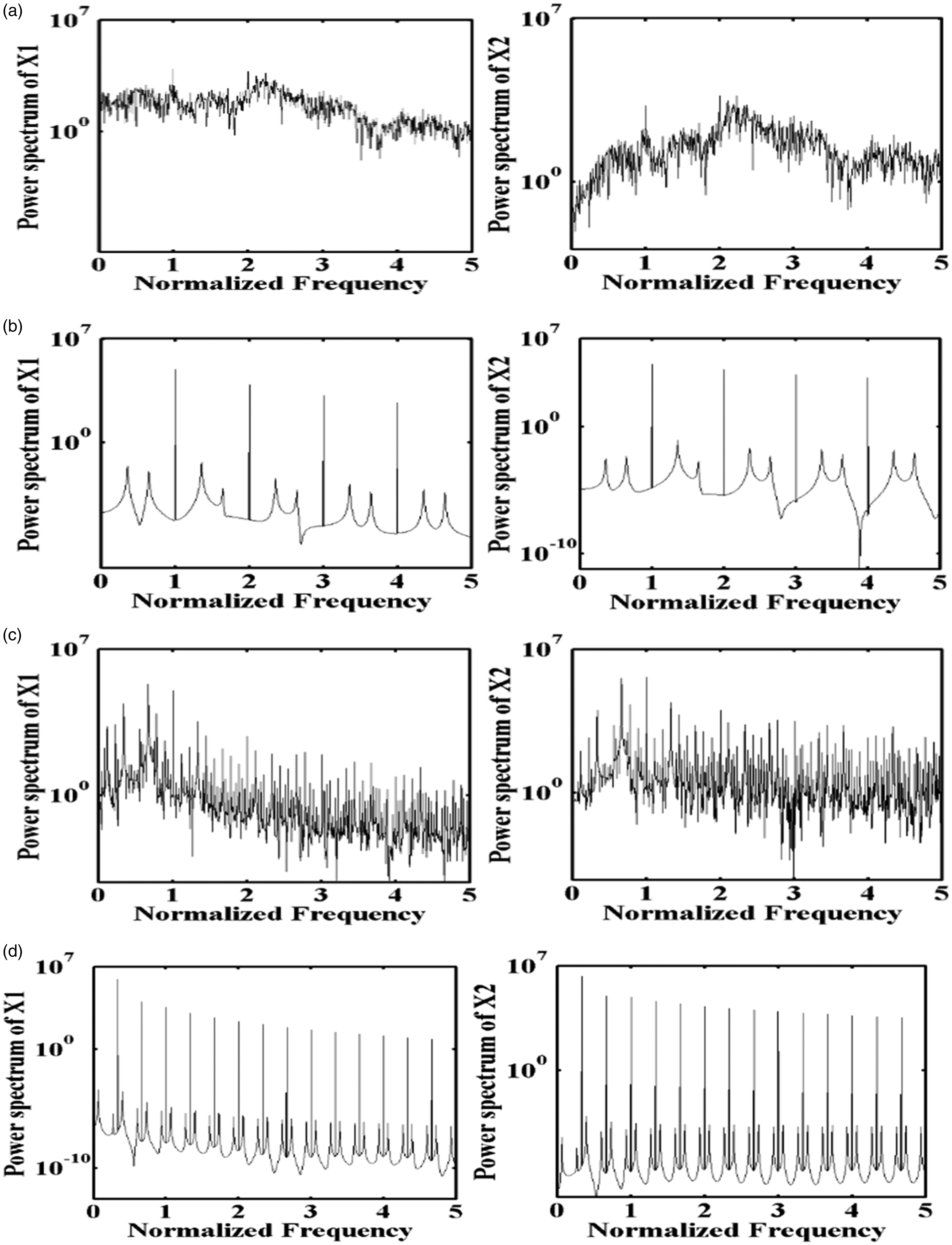
Spectrum analysis of probe tip displacement for (a) Ω = 0.46, (b) Ω = 1.0, (c) Ω = 2.0, and (d) Ω = 3.0.

Bifurcation analysis

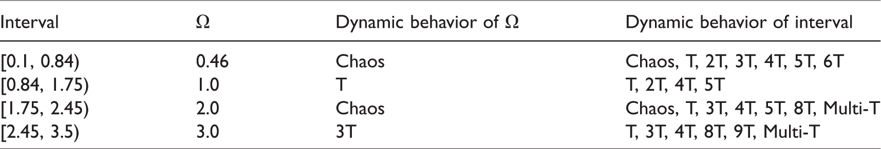
Figure 4 shows a bifurcation diagram of the probe tip displacement and probe tip speed. Observation of the changes in dynamic behavior of the excitation frequency Ω shows two bifurcation diagrams having the same motion behavior, such as T, 2T, 3T, multi-cyclical and non-cyclical behavior. To facilitate subsequent analysis, each motion behavior section was compiled in Table 2 and the dynamic behavior was divided into four regions. The intervals of aperiodic behavior are 0.1 ≦ Ω > 0.84, 1.75 ≦ Ω > 2.45, The rest of the intervals are relatively stable and considered cyclical.

Figure 4.

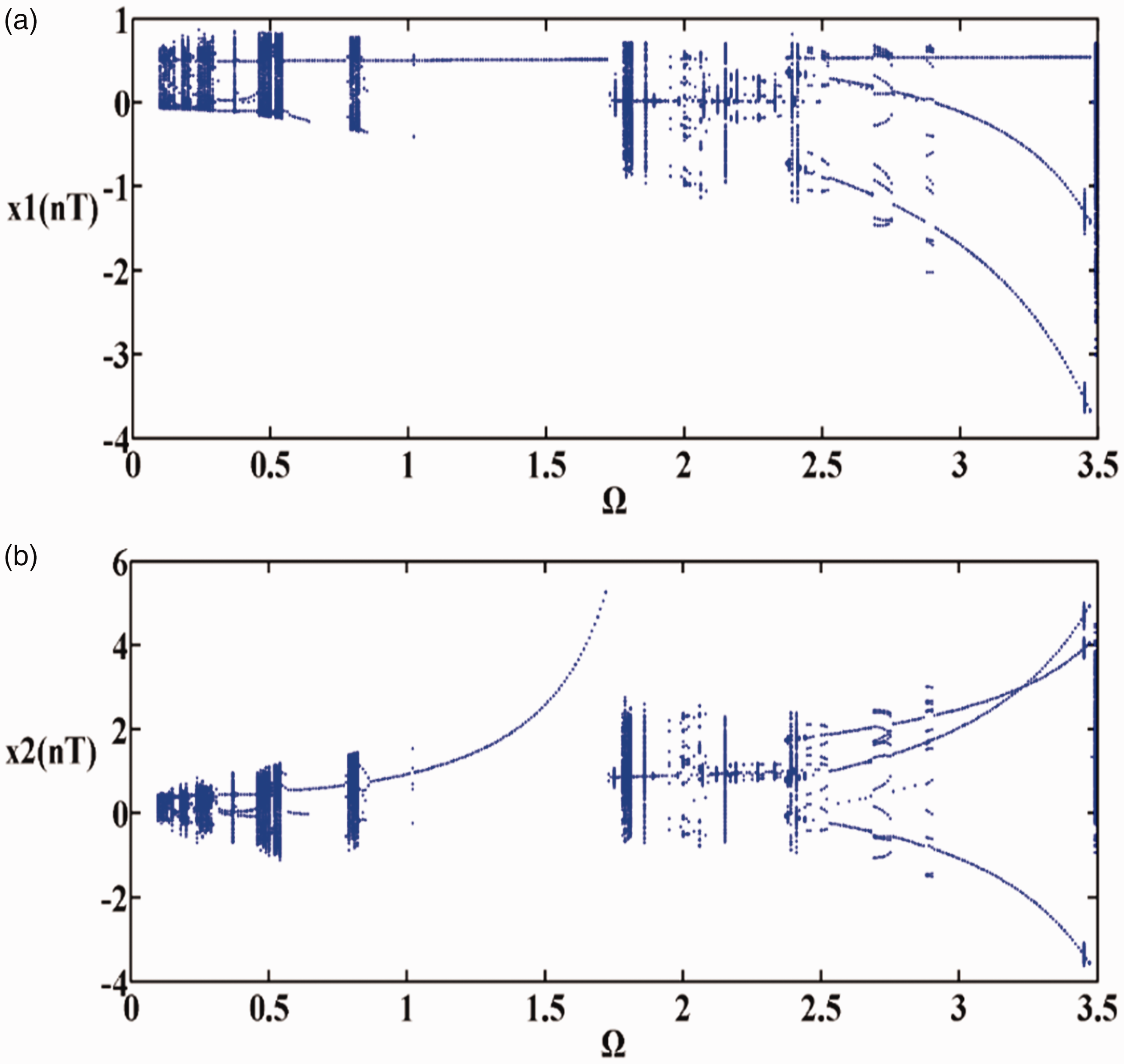
Bifurcation diagrams: (a) probe tip displacement; (b) probe tip speed.

Table 2.

Dynamic interval behavior analysis.

Interval	Ω	Dynamic behavior of Ω	Dynamic behavior of interval
[0.1, 0.84)	0.46	Chaos	Chaos, T, 2T, 3T, 4T, 5T, 6T
[0.84, 1.75)	1.0	T	T, 2T, 4T, 5T
[1.75, 2.45)	2.0	Chaos	Chaos, T, 3T, 4T, 5T, 8T, Multi-T
[2.45, 3.5)	3.0	3T	T, 3T, 4T, 8T, 9T, Multi-T

Any one point can be chosen as representative of any one of the four intervals and used as the main object of the analysis. An examination of the preceding phase plane trajectories and spectral analysis results show Ω = 0.46, 1.0, 2.0, and 3.0 to be in compliance with the findings for chaotic behavior and 1T and 3T as cyclic behavior in bifurcation analysis. After this we used the Poincaré cross-section and the maximal Lyapunov exponent to determine if the dynamic behavior was consistent with the bifurcation results.

Different intervals can be seen and are set out in Table 2. The interval 0.84 ≦ Ω > 1.75, a cyclic 1T motion state, is the most stable.

Poincaré section analysis

The dynamic behavior at Ω = 1.0 is as shown in Figure 5(b). Only one point can be seen in this figure, which also corresponds to a bifurcation. So it can be determined that the dynamic behavior of Ω = 1.0 is the 1T period, and so on. Figure 5(d) coincides with period 3T Ω = 3.0. However, at Ω = 0.46 and Ω = 2.0, the dispersion point shows unstable aperiodic behavior, see Figure 5(a) and (c).

Figure 5.

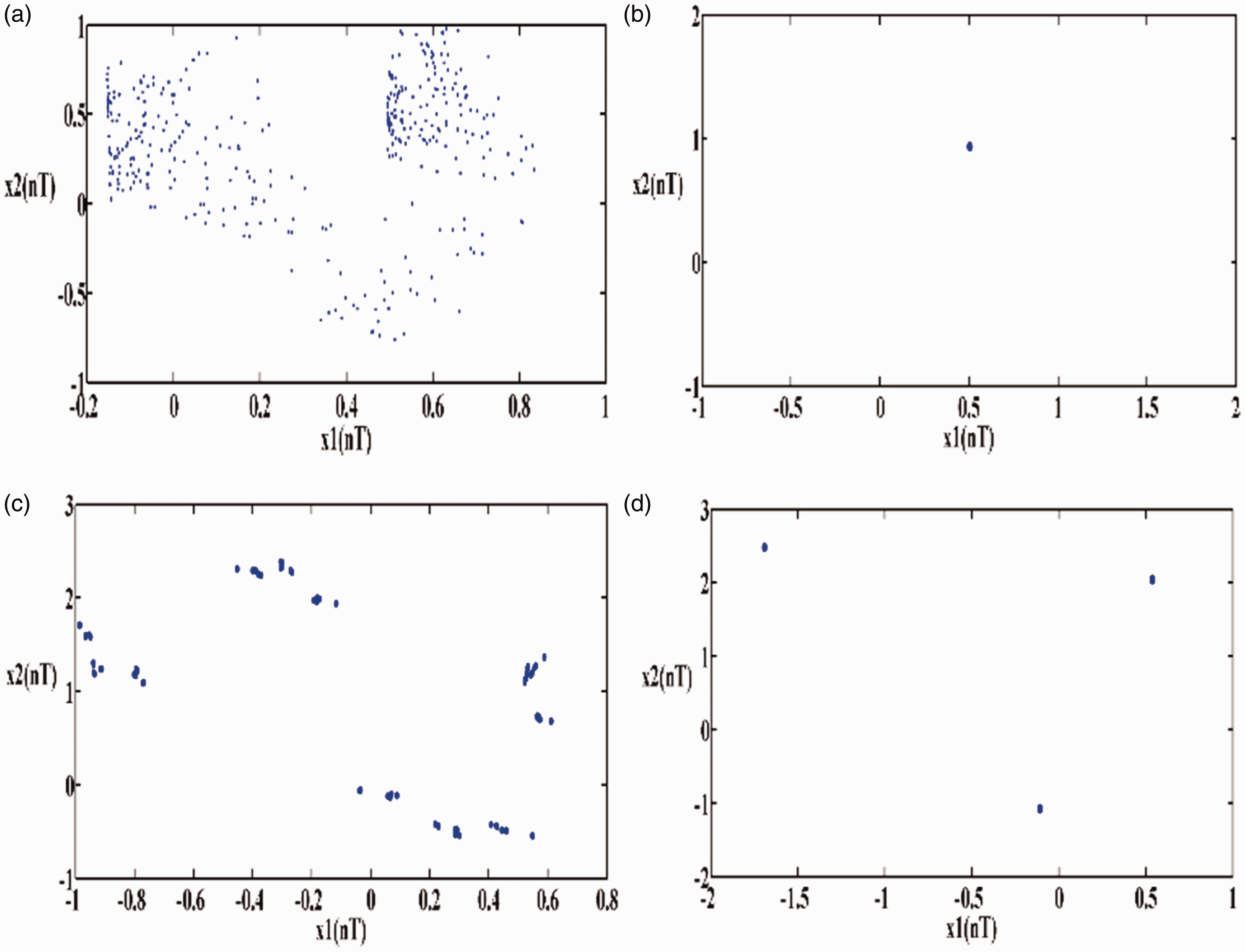
Changes in a sectional view of the probe tip when (a) Ω = 0.46, (b) Ω = 1.0, (c) Ω = 2.0, and (d) Ω = 3.0.

The maximal Lyapunov exponent

The Lyapunov exponent is the most efficient tool for the identification of chaotic behavior. In a quantification system, two infinitely close trajectories in a time series will either converge or diverge at an exponential rate.²⁰ The existence of chaos in a system can be determined by the use of the maximal Lyapunov exponent. When the exponent is less than zero, two adjacent trajectories will eventually merge into a line and a stable system state is indicated by zero. When the exponent is greater than zero, no matter how small the initial interval between two trajectories, this is an indication that as time progresses behavior will become unpredictable at an exponential rate. This is chaotic behavior.

It is clear that for Ω = 0.46, 1.0, 2.0, 3.0, when the exponent is greater than zero, we can be sure that the dynamic behavior will be chaotic, as shown in Figure 6(a) and (c). However, when the stable exponent value is less than, or close to zero, the dynamic behavior will be non-chaotic, as shown in Figure 6(b) and (d).

Figure 6.

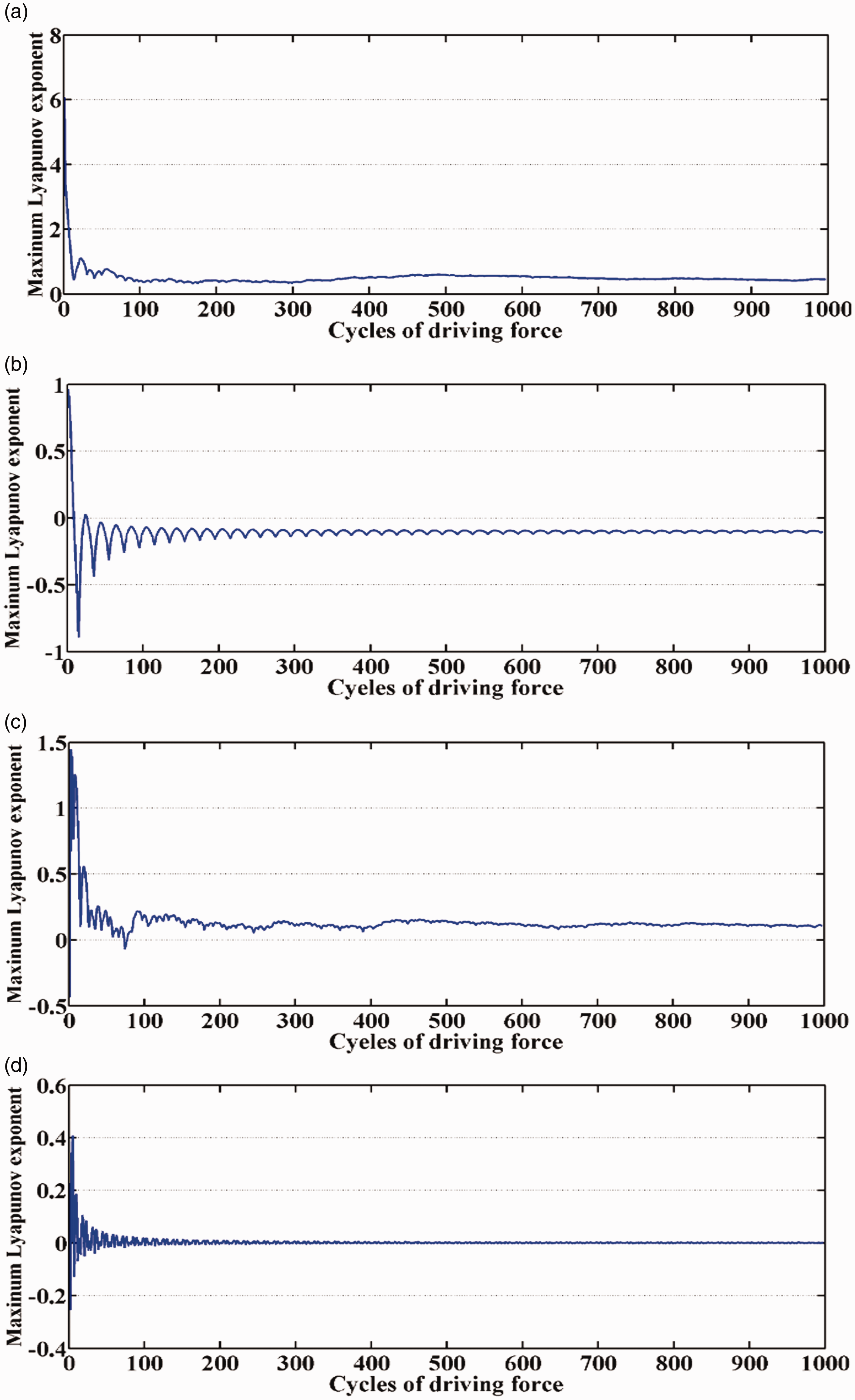
Changes in probe tip maximal Lyapunov exponent for (a) Ω = 0.46, (b) Ω = 1.0, (c) Ω = 2.0, and (d) Ω = 3.0.

Chaos suppression controller

This section describes PD controller design and the fuzzy controller comparison process. Based on dynamic analysis of chaos phenomena in “Dynamic analysis” section, we take excitation frequency Ω = 0.46 as the object for chaos suppression because manual determination of the best controller parameters is quite time-consuming. This section includes an explanation of how PSO and the GA can be used to find, compare, and optimize control parameters K_p and K_D. The PSO and GA fitness function is the integral-absolute-error (IAE) for the system dynamic error e(t), which converges on a minimum value as a parameter search performance index, and allows the AFM system output response y(t) to suppress irregular behavior, as shown in the block diagram in Figure 7.

Figure 7.

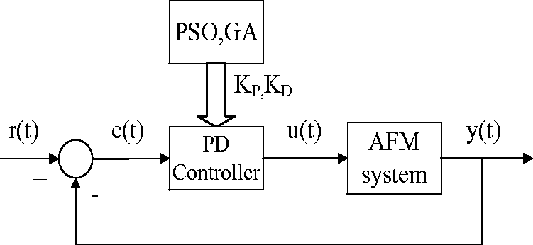
A PSO block diagram for finding the optimal PD control parameters. AFM: atomic force microscope; GA: genetic algorithm; PD: proportional-derivative; PSO: particle swarm optimization.

System mathematical model with PD controller

First, to suppress AFM system chaos, we set the input reference term $r(t)$ as the constant term zero, so that the output response y(t) of the system could be inhibitory. As the system dynamic error approaches zero, the control term u(t) is added to equation (5) to obtain the following

{\dot{X}}_{1} = X_{2}

(4)

\begin{matrix} {\dot{X}}_{2} = - S_{1} X_{2} - X_{1} + S_{2} + \frac{S_{3}}{{(1 - X_{1} - S_{6} \sin (Ω τ))}^{8}} \\ + \frac{S_{4}}{{(1 - X_{1} - S_{6} \sin (Ω τ))}^{2}} + S_{5} Ω^{2} S_{6} \sin (Ω τ) + u (t) \end{matrix}

(5)

To ensure the dynamic error $[e_{1}, e_{2}]$ is close to zero, the system output term y(t) is subtracted from the input reference term r(t), as shown in equation (6). The dynamic error is obtained from the PD control term u(t), as in equation (9), where the formula to meet the condition is as follows

\lim_{t \to \infty} | | r_{i} (t) - y_{i} (t) | | = \lim_{t \to \infty} | | e_{i} (t) | | \to 0, i = 1, 2

(6)

To meet the conditions and find the dynamic error, substitute $e (t) = (r_{1} (t) - y_{1} (t), r_{2} (t) - y_{2} (t)) = (e_{1}, e_{2})$ into equations (7) and (8), then the following equation can be derived

{\dot{e}}_{1} = e_{2}

(7)

\begin{matrix} {\dot{e}}_{2} = - S_{1} e_{2} - e_{1} + S_{2} + \frac{S_{3}}{{(1 - X_{1} - Z \sin (Ω τ))}^{8}} \\ + \frac{S_{4}}{{(1 - X_{1} - Z \sin (Ω τ))}^{2}} + Z Ω^{2} S_{5} \sin (Ω τ) + u (t) \end{matrix}

(8)

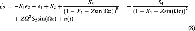
Wherein the control term u(t) is as follows

u (t) = K_{P} e_{1} + K_{D} e_{2}

(9)

System response characteristic assessment

The system is searched for optimal parameters using PSO and GA. There is a need for a fitness function to compare the merits and drawbacks of the parameter, so the fitness function used as the basis for assessing the parameters is the IAE of the dynamic error e₁. The equation is as follows

I A E = \int_{0}^{\infty} | e_{1} (t) | d t

(10)

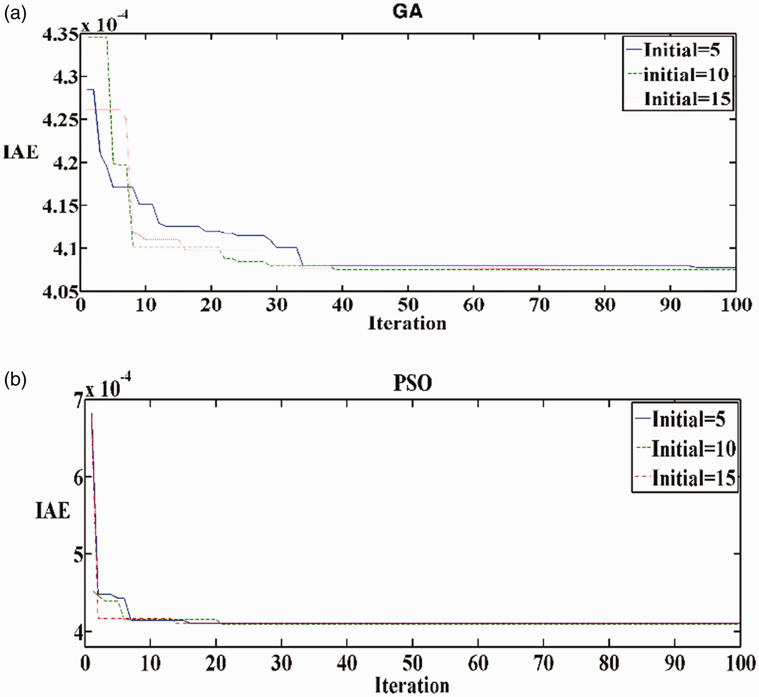
A comparison of the IAE of the two algorithms shows that PSO will converge to stability after 20 to 30 iterations, while GA needs about 40 iterations, or even more, to reach stability. To save time the follow-up parameter searches were mostly done using PSO.

PSO and GA optimization parameters search

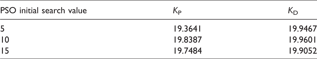
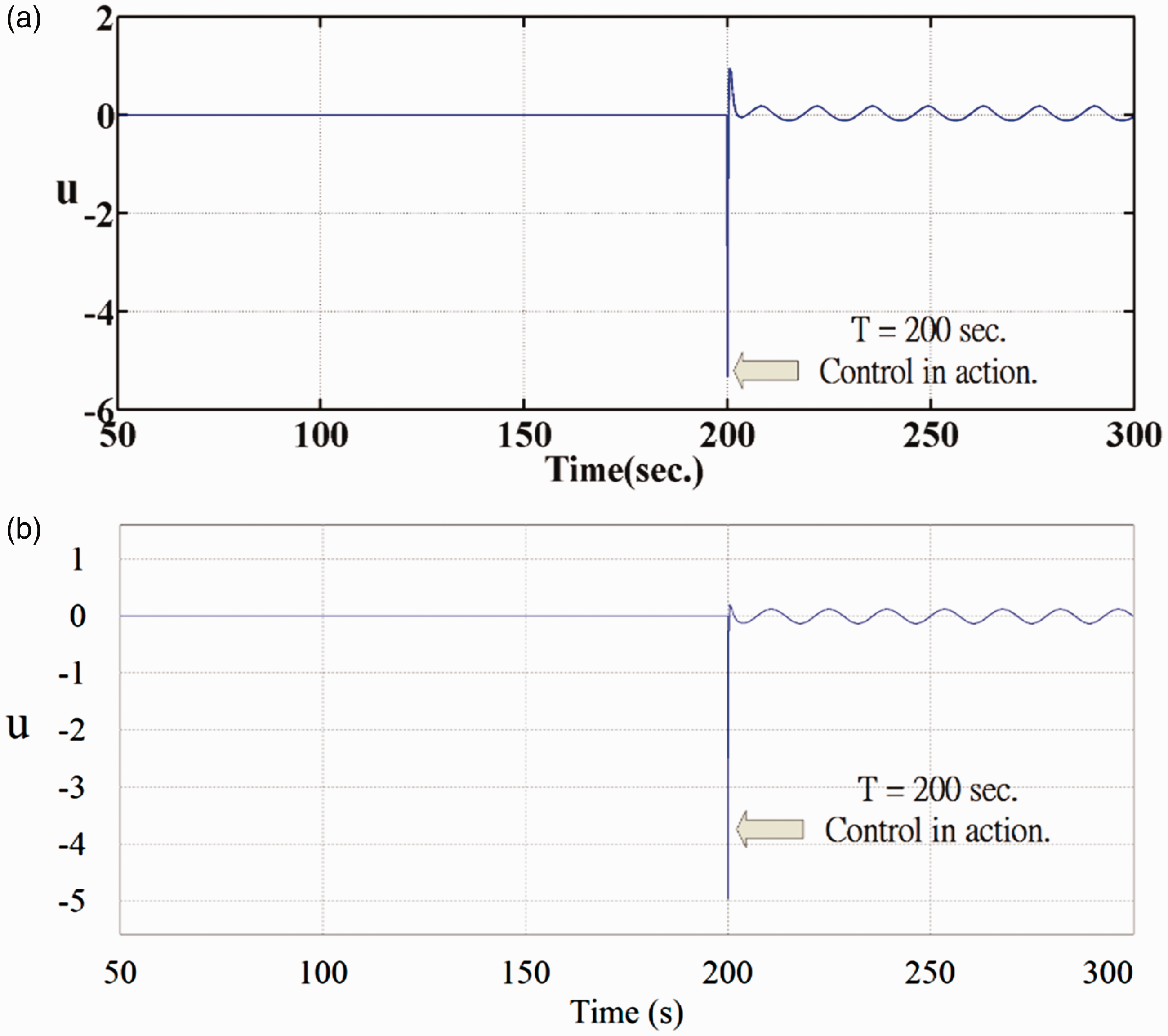
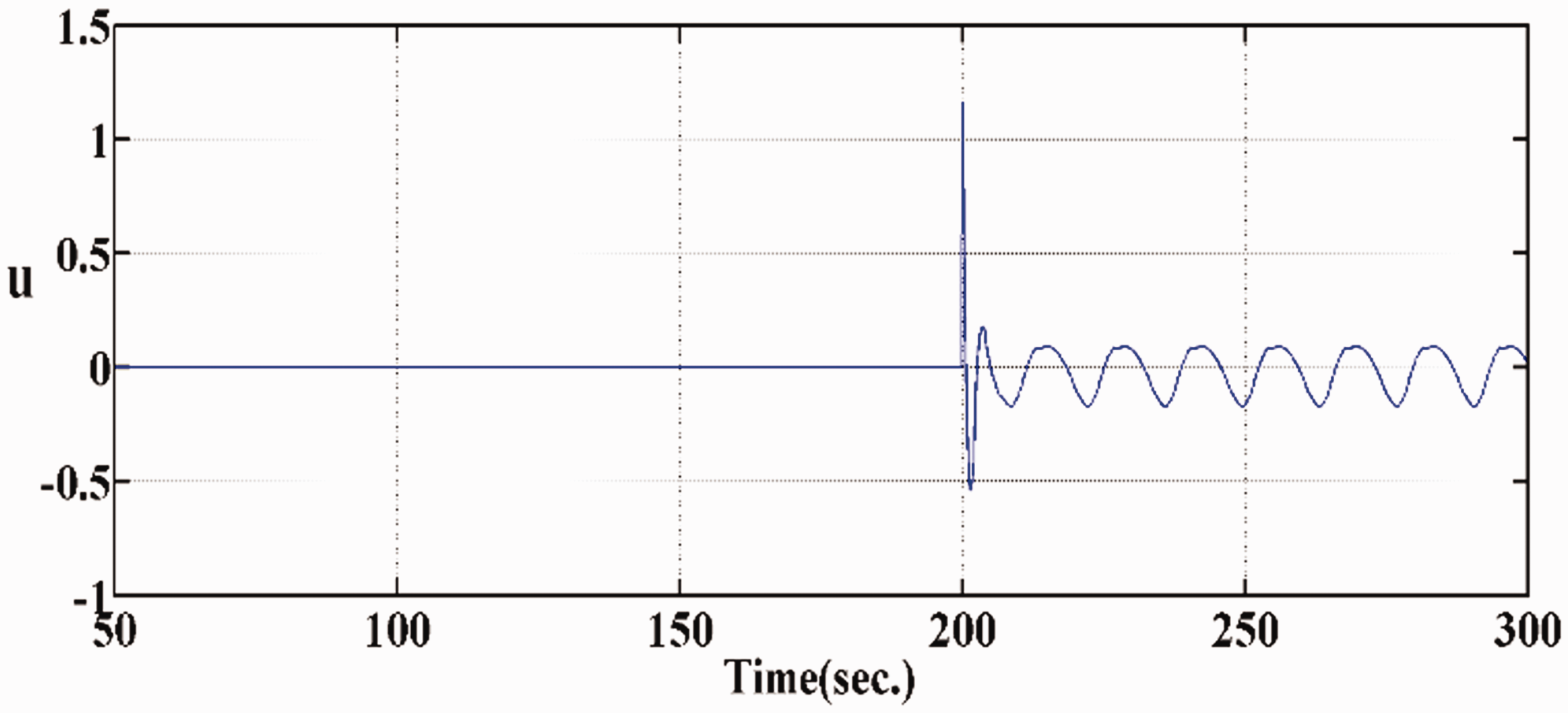
To realize an actual circuit use ±12 V as an actual limit to prevent errors at implementation, then consider the control term u(t) as being limited to 10 or less. To avoid saturation of the hardware circuit, we substituted parameters K_p=19.3641 and K_D=19.9467 obtained from Table 3 into the control term resulting from PD control u(t), as shown in Figure 8.

Table 3.

PSO and GA parameters search results.

PSO initial search value	K_P	K_D
5	19.3641	19.9467
10	19.8387	19.9601
15	19.7484	19.9052

Figure 8.

(a) Matlab/Simulink; (b) Psim circuit simulation control term u time response.

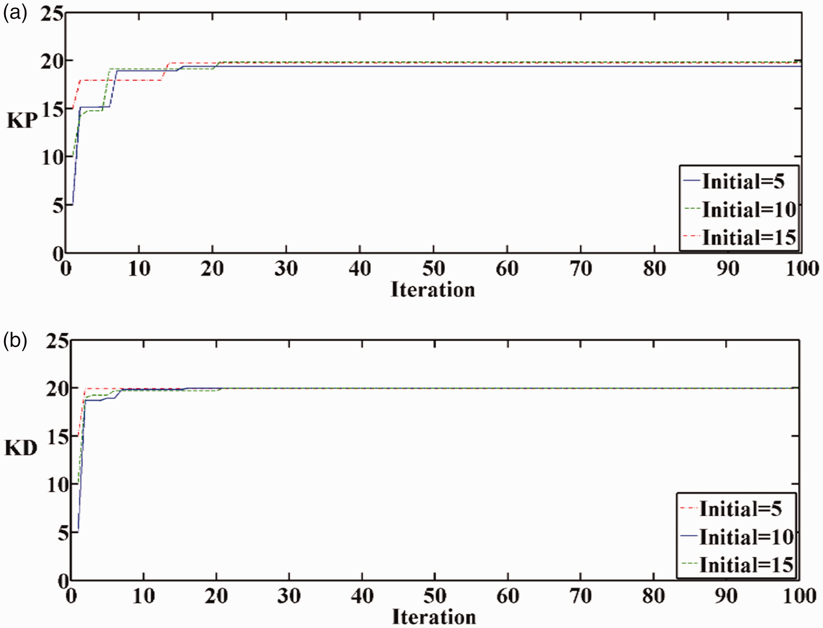
The search range for parameters K_p and K_D is limited to 0 to 20, and the initial values for the search for parameters K_p and K_D were set to 5, 10, and 15, this proved the robustness of PSO searches as shown in Figure 9(a) and (b). It was found that the best convergence for PSO occurred between 20 and 30 iterations. This corresponds to the IAE of the fitness function in Figure 10(b), which shows consistent results.

Figure 9.

(a) Search parameter K_p iteration trace; (b) search parameter K_D iteration trace.

Figure 10.

Comparison of the IAE fitness function (a) GA and (b) PSO. GA: genetic algorithm; IAE: integral-absolute-error; PSO: particle swarm optimization.

The results showed that even if the initial values are different, those obtained for the AFM system optimal control parameters are very close to each other as can be seen in Table 3.

PD control simulation and experimental results

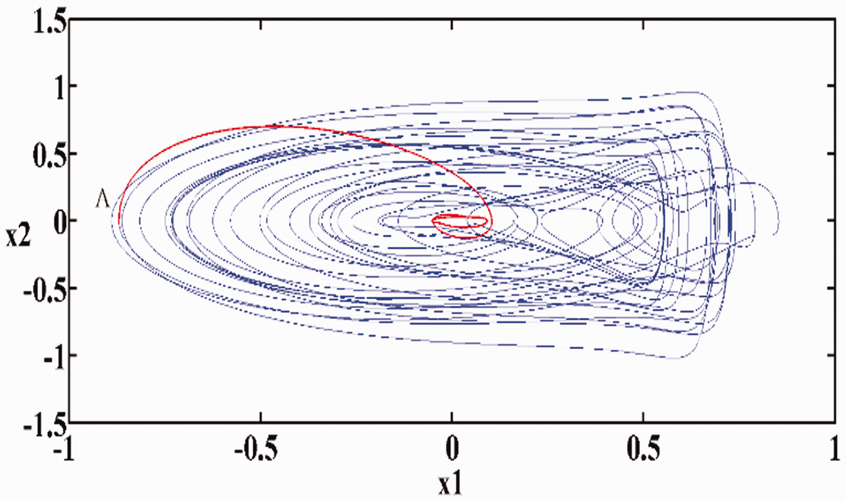
In this section, the excitation frequency Ω = 0.46 which gives chaotic behavior was chosen as the objective for control. The corresponding chaotic phase plane trajectories are as shown in Figure 2(a). Psim circuit simulation software was used to design an AFM system differential circuit and the Ω = 0.46 chaotic phase flat trajectory is shown in Figure 11(a). The Psim simulation results are consistent with those of the previous dynamic analysis and have the same irregular chaotic trajectory. After control was added at time A on the system phase plane trajectory, the trajectory converged to a point very near zero. This clearly shows that stability was achieved by suppression of chaotic motion as can be seen in the phase plane trajectory trace. Control results are shown on the phase plane trajectory of the system in Figure 11.

Figure 11.

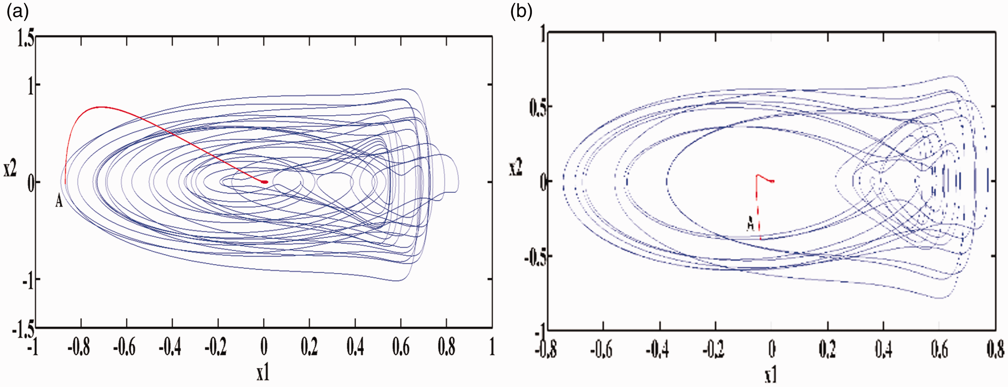
(a) Matlab/Simulink; (b) phase plane trajectories after PD control was added to the Psim circuit simulation.

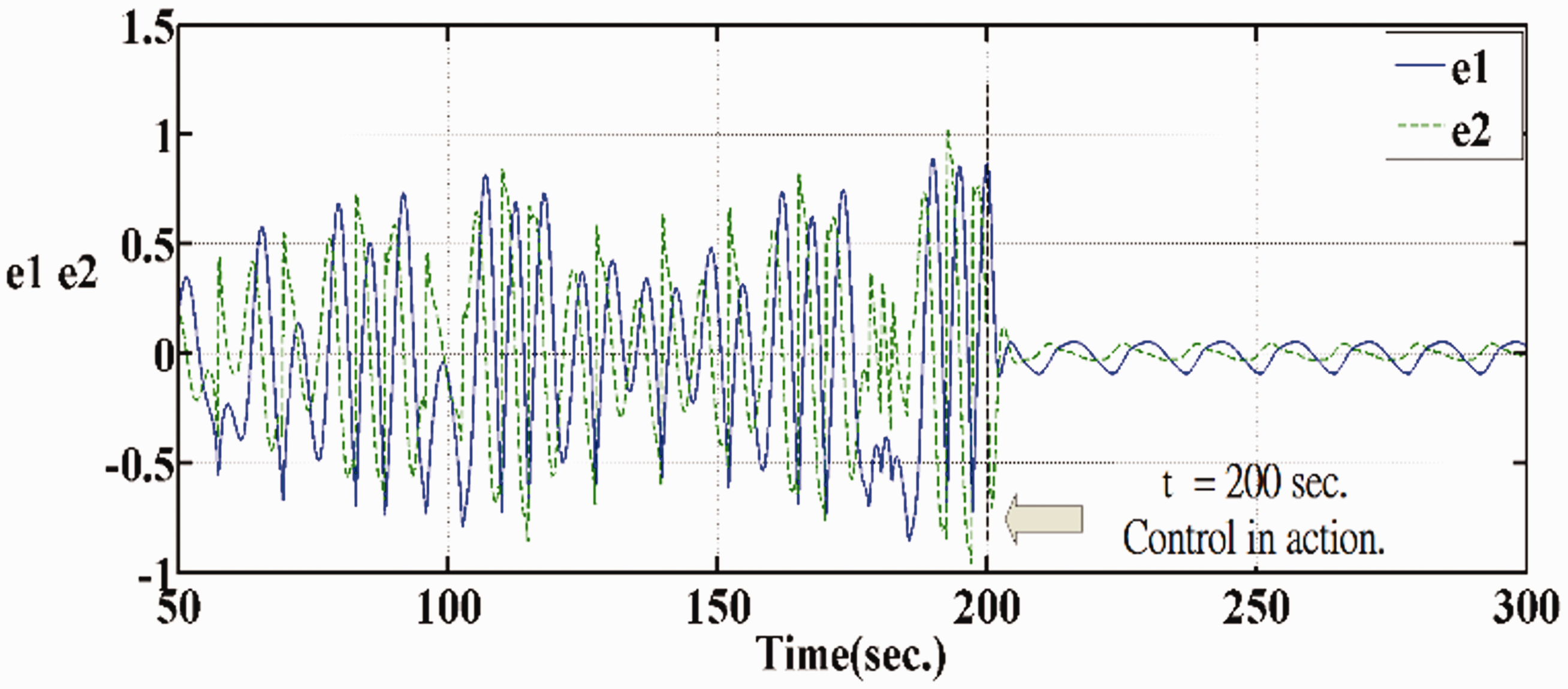
The effect of control can also be observed in the suppression of dynamic errors e₁ and e₂ in a time response diagram. Figure 12 shows a 300-s long trace of an AFM simulation with chaotic behavior where the value of dynamic errors e₁ and e₂ fluctuate widely. After 200 s of simulation of chaotic behavior, PD control was started and by second 205 the fluctuations had been suppressed and the system was stable. The effect of control can be clearly seen in Figure 12.

Figure 12.

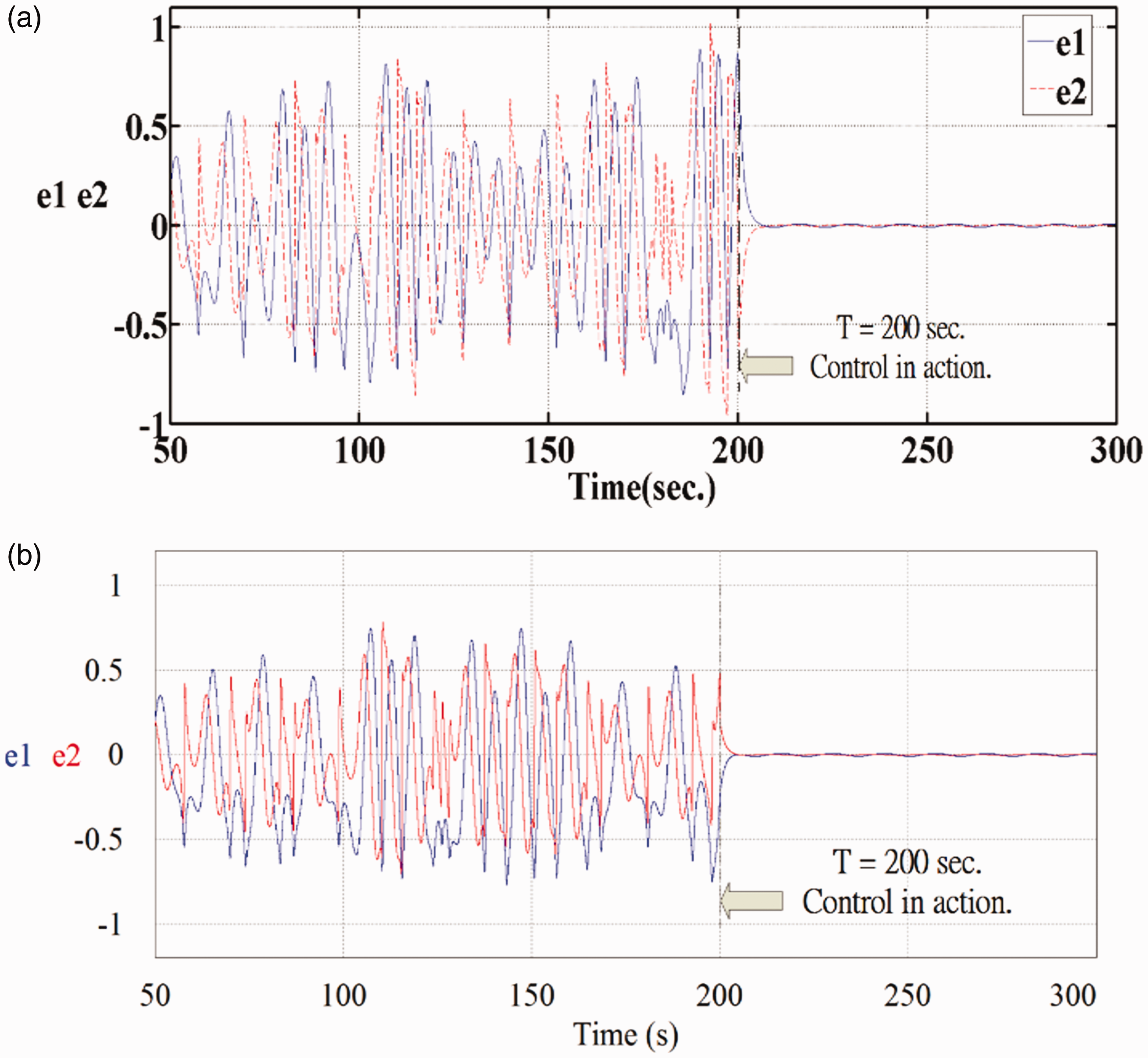
(a) Matlab/Simulink. (b) Time response trace for Psim circuit simulation showing suppression of dynamic errors e₁ and e₂ by PD control.

Fuzzy controller design

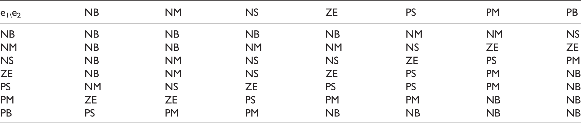
Matlab/Simulink was used to add fuzzy control to an AFM system simulation. The membership function of e₁ and e₂ was confined to a range between −20 and 20. Table 4 shows the fuzzy control rules which are: negative big (NB), negative medium (NM), negative small (NS), zero (ZE), positive small (PS), positive medium (PM), and positive big (PB).

Table 4.

Fuzzy control rules.

e_1\e₂	NB	NM	NS	ZE	PS	PM	PB
NB	NB	NB	NB	NB	NM	NM	NS
NM	NB	NB	NM	NM	NS	ZE	ZE
NS	NB	NM	NS	NS	ZE	PS	PM
ZE	NB	NM	NS	ZE	PS	PM	NB
PS	NM	NS	ZE	PS	PS	PM	NB
PM	ZE	ZE	PS	PM	PM	NB	NB
PB	PS	PM	PM	NB	NB	NB	NB

The chaotic behavior at Ω = 0.46 was taken as the object of control and the phase plane trajectory after control has been added is shown in Figure 13. Control is added at time A, the irregular trajectory is suppressed and the trace settles at a point near zero.

Figure 13.

Phase plane trajectories after the addition of fuzzy control.

The dynamic errors e₁ and e₂ on the time response diagram show the effect of control. Control starts at second 200 and by second 210 stability has been achieved, see Figure 14.

Figure 14.

Dynamic errors e₁ and e₂ time response graph with fuzzy control added.

A comparison of fuzzy control with PD shows PD to have better control, but it has a higher surge, as shown in Figure 15.

Figure 15.

Fuzzy control term u time response graph.

AFM system circuit design

We chose circuit simulation excitation frequencies of Ω = 1.0 and Ω = 0.46 to include systems with both periodic and aperiodic behavior. The phase plane trajectory diagram of a Psim simulation of an AFM system is shown in Figure 16(a) and (b). The phenomena are consistent with the dynamic analyses dealt with in “Dynamic analysis” section and it can be clearly seen that different excitation frequencies affect the dynamic behavior of the AFM probe.

Figure 16.

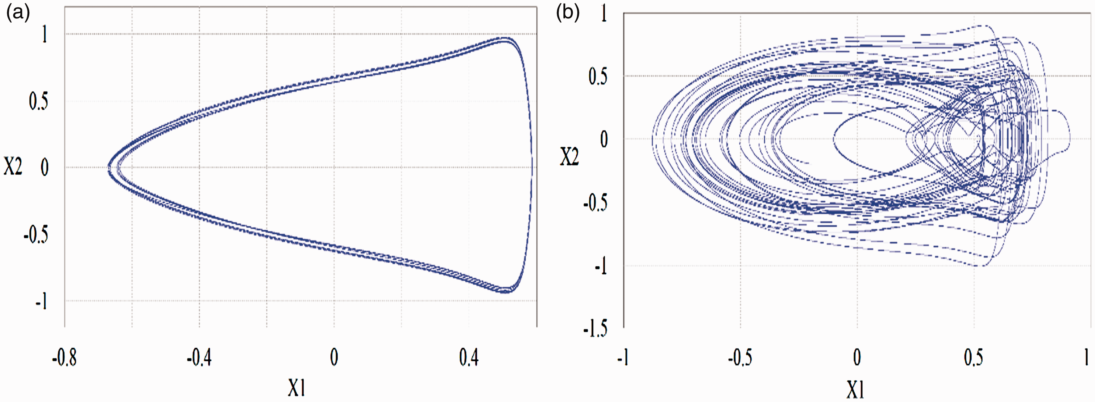
Phase plane trajectory diagrams of the Psim simulation of probe tip (a) Ω = 1.0; (b) Ω = 0.46.

Hardware circuit realization

Observations of the phase plane trajectories generated by an actual hardware circuit, displayed on an oscilloscope, showed similar behavior. Oscilloscope channel 1 was probe displacement X₁ and channel 2 was speed X₂ (the oscilloscope was in XY mode). Figure 17(a) and (b) is phase plane trajectories traces at the excitation frequencies Ω = 1.0 and Ω = 0.46. These trajectories, showing both periodic and aperiodic behavior, are consistent with the dynamic analysis results.

Figure 17.

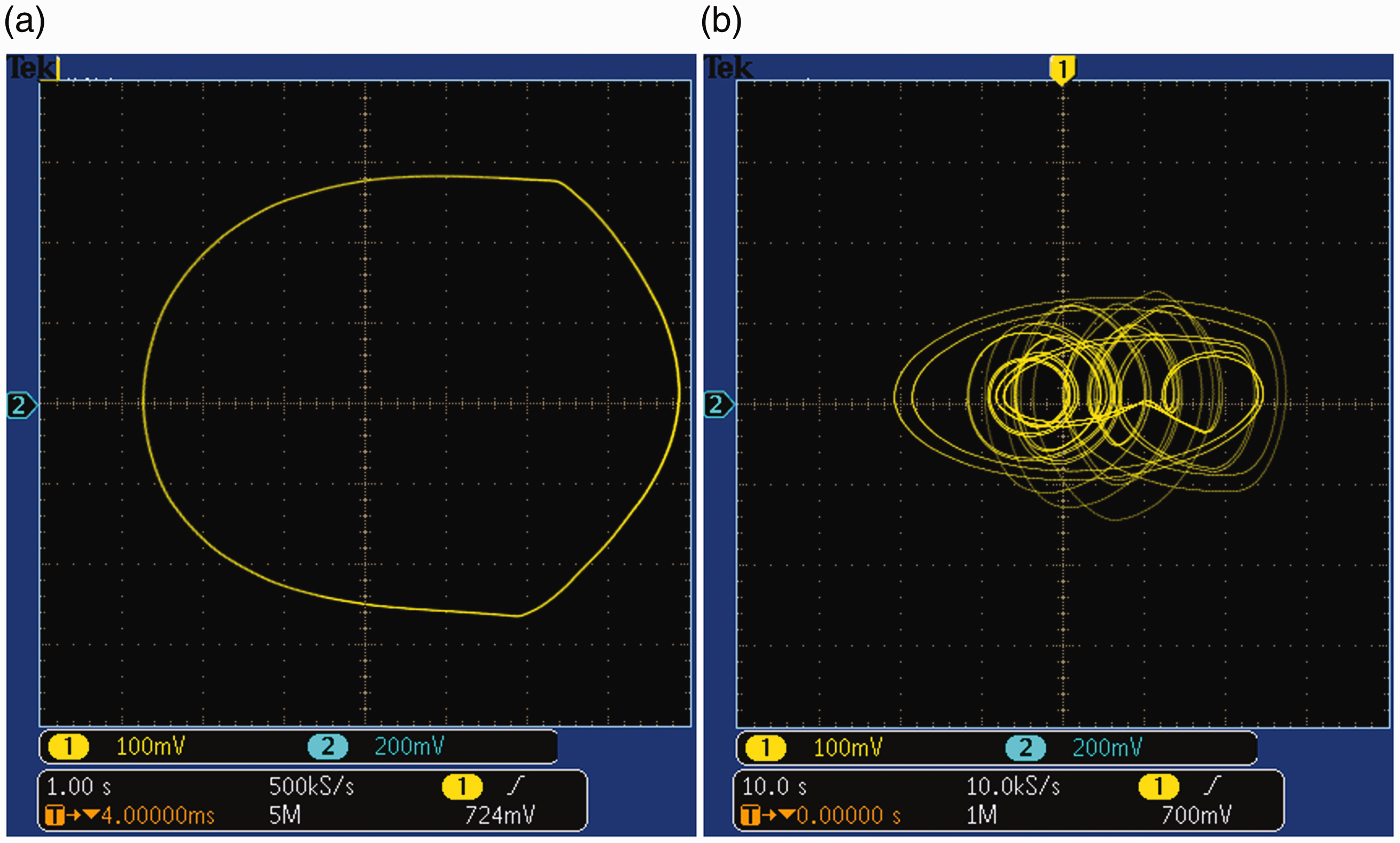
(a) Ω = 1.0; (b) Ω = 0.46 are oscilloscope traces of phase plane trajectories diagrams (X₁ and X₂) generated by the hardware circuit.

Spectrum analysis and maximal Lyapunov exponent analysis were carried out on data captured by the oscilloscope for use in dynamic analysis. By validation of these tools, it can be shown that the phenomena generated by hardware circuits are in line with what we call periodic and aperiodic behavior, as shown in Figures 18 and 19. The results obtained from the two different analysis tools are consistent and explain why differences in excitation frequency can cause chaotic behavior in an AFM system.

Figure 18.

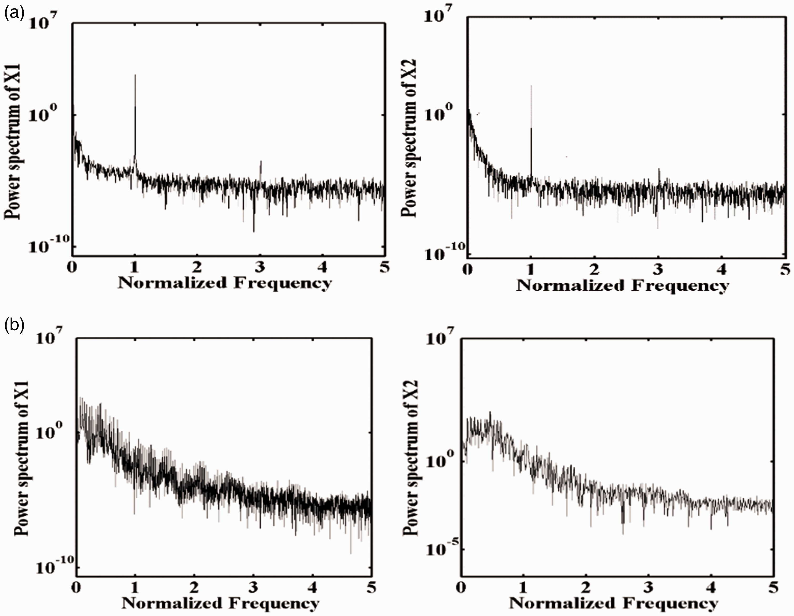
(a) Ω = 1.0 and (b) Ω = 0.46 are the spectral analysis diagrams for the hardware circuit X₁ and X₂.

Figure 19.

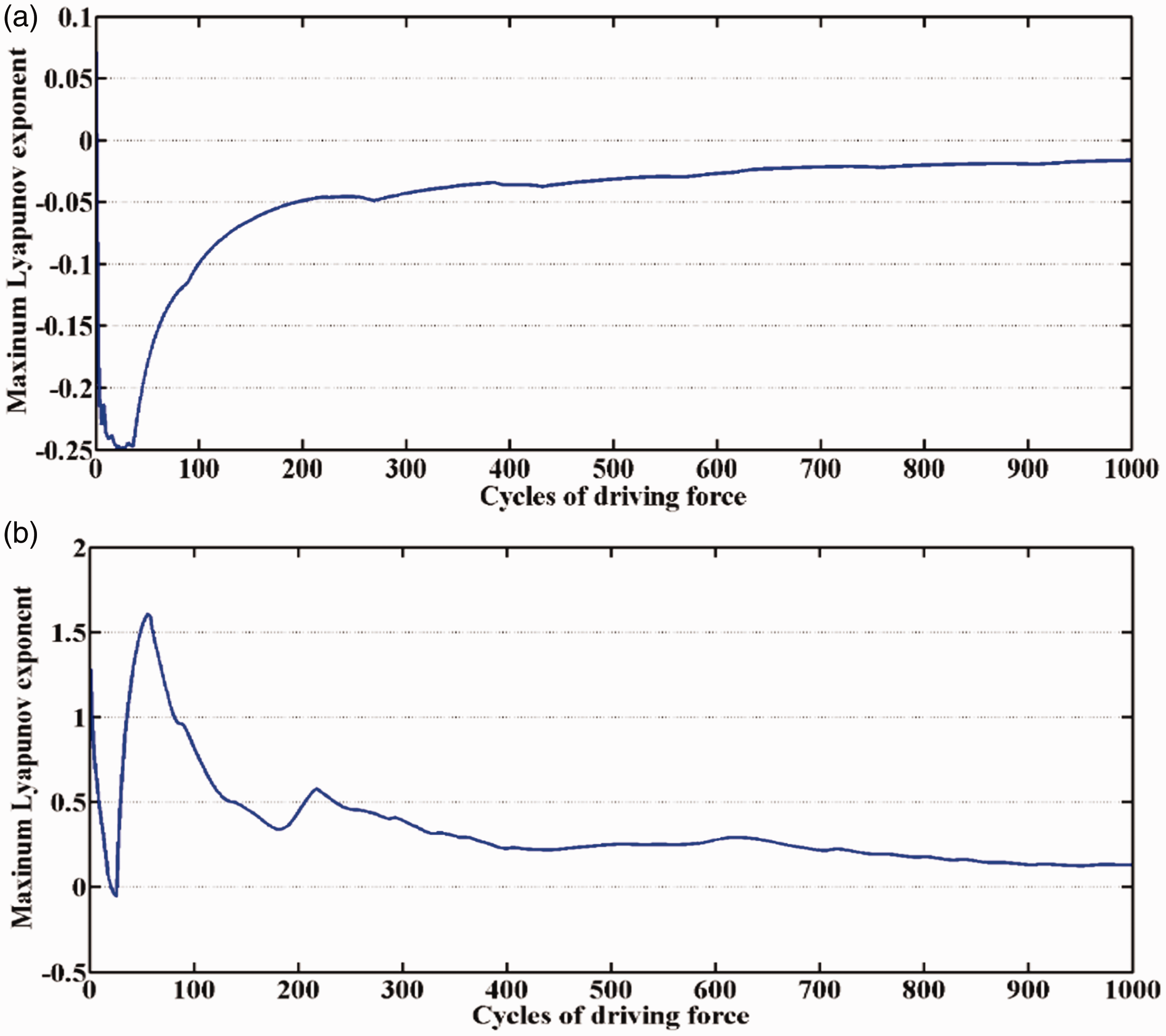
The maximal Lyapunov exponent for the hardware circuit X₁ and X₂. (a) Ω = 1.0 (b) Ω = 0.46.

Experimental results for the hardware circuit with added PD control

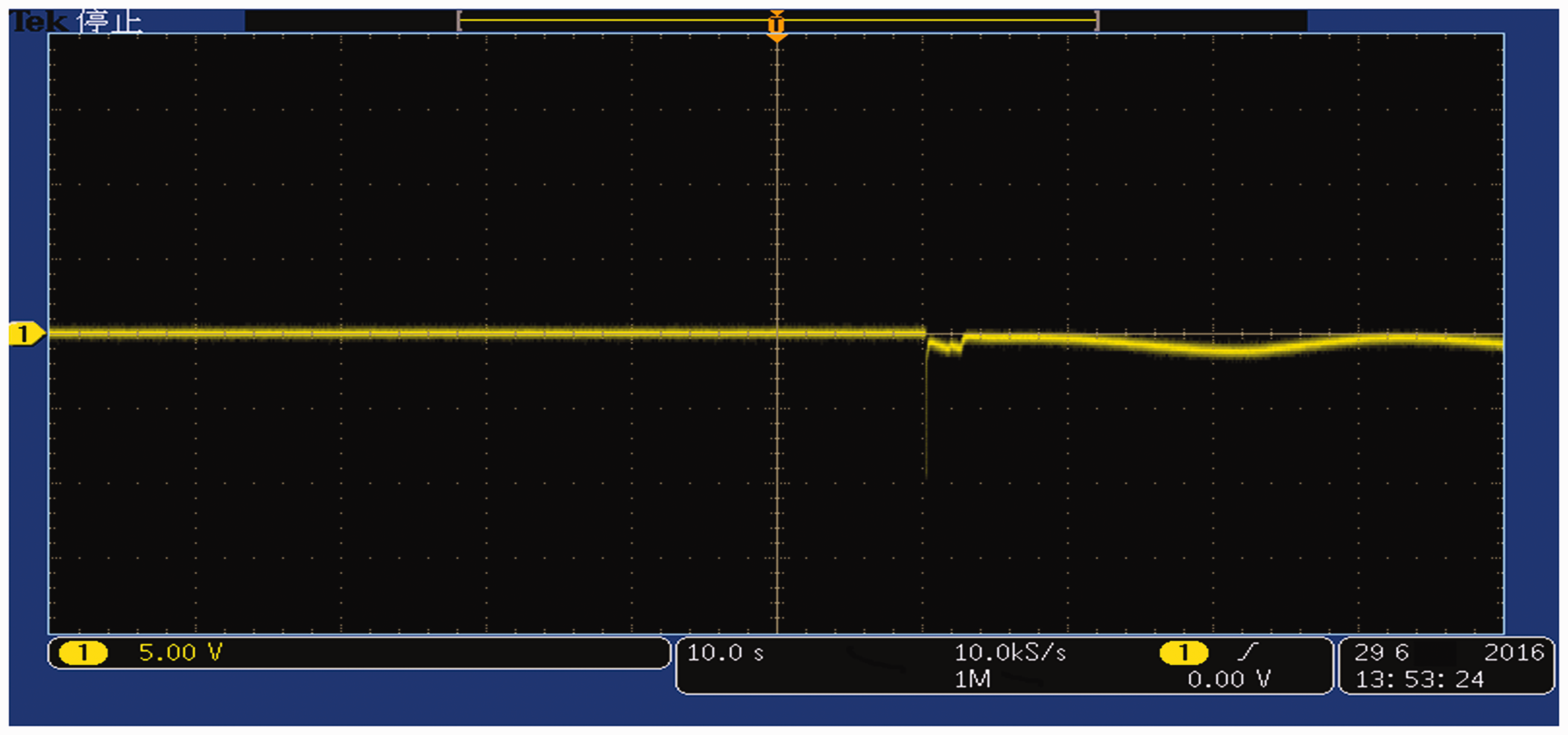
The validation of these tools shows that with the same parameters an AFM hardware circuit will exhibit the same chaotic behavior as a simulation. Therefore, to suppress chaotic behavior in the circuit, we add a hardware PD controller. The control parameters K_p and K_D are fine-tuned by precision variable resistors in the circuit in accordance with controller design and the parameter search results in the previous section. The effects of control can be observed in the dynamic error e₁ and e₂ time response curve, shown in Figure 20. Channel 1 and channel 2 are dynamic errors e₁ and e₂, respectively. Control can be added at any time after the waveform reaches a steady state. The waveforms e₁ and e₂ become stable at 0 V within about 5 s.

Figure 20.

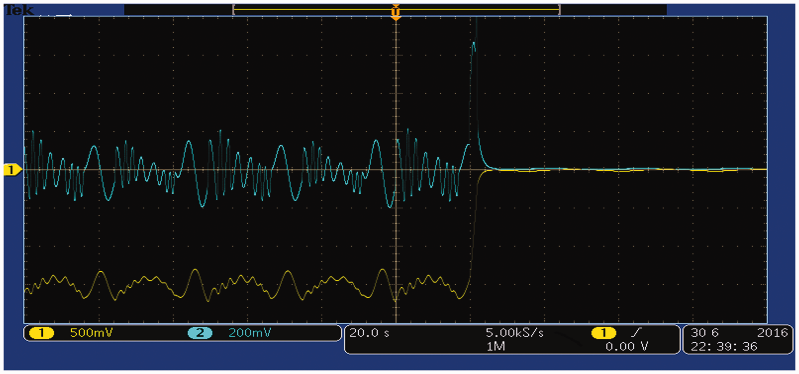
The time response curve after PD control has been added.

It was mentioned earlier that the control term u might cause operating voltage saturation if the control parameters K_p and K_D were excessive. Using K_p=19.3641 and K_D=19.6467 control was added at any time, resulting in the control u time response waveform shown in Figure 21. At the instant when control was added a surge voltage of about −10 V was observed, which was within the expected range.

Figure 21.

Hardware circuit PD control u time response curve.

Hardware circuit experimental results after the addition of fuzzy control

The computer terminal binding Matlab/Simulink to the real-time interface (RTI) was used in the design of the fuzzy controller. The hardware circuit waveform signal from the AFM system was transferred by the ADC via a CLP1104 signal connector to a computer terminal that used dSPACE control. The effects of control were observed on an oscilloscope, see Figure 22. Channels 1 and 2 show waveform traces of the dynamic errors e₁ and e₂, respectively. The waveforms stabilized at around 0 V within about 10 s after control was applied, as shown in Figure 22(a).

Figure 22.

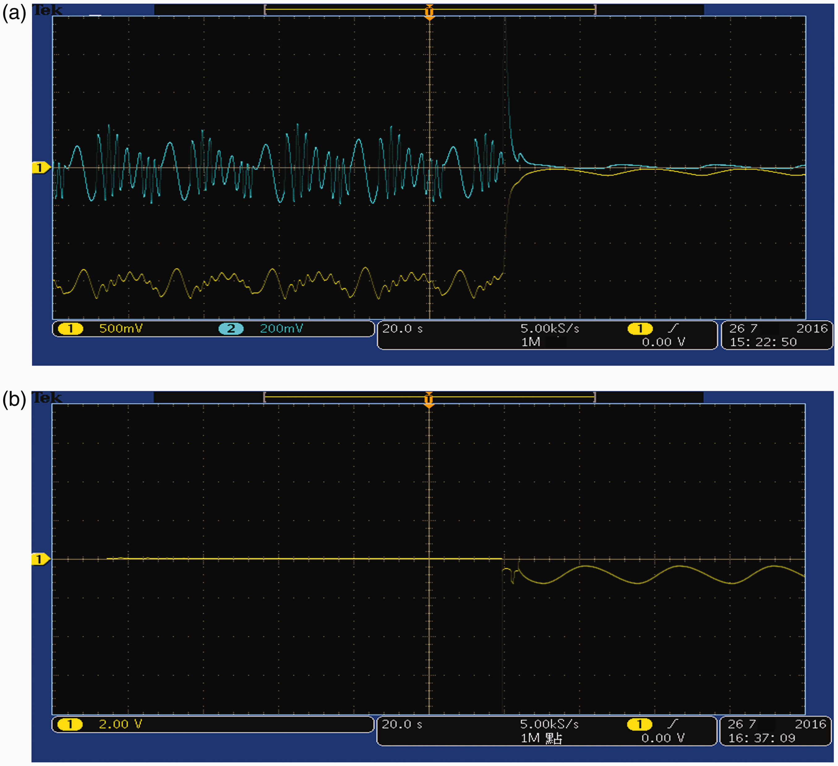
(a) e₁ and e₂ time response graph after fuzzy control is added to the hardware circuit; (b) fuzzy control u time response graph.

The fuzzy controller had a voltage surge of about −4 V which was smaller than that of the PD controller. After stabilization the waveform amplitude variations were not only larger, but also stable at around 0 V, as shown in Figure 22(b).

Conclusions

In this study the nonlinear behavior of an AFM caused by changes in excitation frequency was investigated. Numerical analysis showed that the tools used for analysis gave consistent results and changes of excitation frequency have significant effect on behavior of the system. The nonlinear behavior of the system caused by different excitation frequency was set out in a table that clearly shows the difference between periodic and aperiodic behavior. The results can be used as a guideline or future reference to determine AFM system adjustment parameters and to improve system measurement accuracy especially where the chaotic motion occurs in two specific intervals.

To control the chaos efficiently, a chaos suppression controller was developed and PSO and the GA were used to find, compare, and optimize the control parameters. The PSO and GA fitness function was the IAE, converging on a minimum value, used as a parameter search performance index. This allowed the AFM system to successfully suppress irregular chaotic behavior.

The Psim circuit simulation results were applied to verify the numerical analysis results. It was found that these two results were identical and correct. This confirmed that the chaotic behavior in the hardware system was the same as in the simulation. The PD and fuzzy control were both implemented in an AFM system and the results were compared. It was found that the control established by both Matlab/Simulink and Psim circuit simulations could inhibit chaotic behavior efficiently. Verification of the results of numerical analysis and Psim circuit simulation was made in actual physical AFM hardware circuitry where both periodic and aperiodic phenomena were observed. The hardware implementation of PD and fuzzy control not only readily suppressed irregular trajectory traces but also confirmed the validity of the PSO parameter search procedure. The hardware circuit design and controller proposed in this paper efficiently suppressed chaotic behavior and can be applied to real AFM systems.

Footnotes

The author(s) declared no potential conflicts of interest with respect to the research, authorship, and/or publication of this article.

Funding

The author(s) disclosed receipt of the following financial support for the research, authorship, and/or publication of this article: the Ministry of Science and Technology of the ROC, under projects No. 106-2221-E-167-012-MY2, 106-2218-E-167-001 & 106-2622-E-167-010-CC3.

References

Roy

Chen

Cong

, et al. A semi-automated positioning system for contact-mode atomic force microscopy (AFM). IEEE Trans Autom Sci Eng 2013; 10: 462.

Pishkenari

Mahboobi

Meghdari

Hybrid finite-element method-molecular dynamics approach for modelling of non-contact atomic force microscopy imaging. IET Micro Nano Lett 2011; 6: 412.

Rabe

Janser

Arnold

Vibrations of free and surface-coupled atomic force microscope cantilevers: theory and experiment. Rev Sci Instrum 1996; 67: 3281.

Sader

JE.

Frequency response of cantilever beams immersed in viscous fluids with applications to the atomic force microscope. J Appl Phys 1998; 84: 64.

Aimé

Couturier

Boisgard

, et al. Relationship between the non linear dynamic behaviour of an oscillating tip-microlever system and the contrast at the atomic scale. Appl Surf Sci 1999; 140: 333.

Ashhab

Salapaka

Dahleh

, et al. Dynamical analysis and control of microcantilevers. Automatica 1999; 35: 1663.

Ashhab

Salapaka

Dahleh

, et al. Melnikov-based dynamical analysis of icrocantilevers in scanning probe microscopy. Nonlinear Dyn 1999; 20: 197.

Rützel

Lee

Raman

Nonlinear dynamics of atomic-force-microscope probes driven in Lennard–Jones potentials. Philos Trans R Soc London Ser A 2003; 459: 1925.

Burnham

Colton

Pollock

HM.

Interpretation of force curves in force microscopy. Nanotechnology 1993; 4: 64.

10.

Burnham

Kulik

Gremaud

, et al. Nanosubharmonics: the dynamics of small nonlinear contacts. Phys Rev Lett 1995; 74: 5092.

11.

Oveisi

Gudarzi

Adaptive sliding mode vibration control of a nonlinear smart beam: a comparison with self-tuning ziegler-nichols PID controller. J Low Freq Noise Vib Active Control 2013; 32: 41.

12.

Sun

, et al. Active vibration control of a conical shell using piezoelectric ceramics. J Low Freq Noise Vib Active Control 2017; 36: 366.

13.

Wang

YJ.

Constant force feedback controller design using PID-like fuzzy technique for tapping mode atomic force microscopes. Intell Control Autom 2013; 4: 17.

14.

Lee

GZ.

A particle swarm optimization approach for optimum design of PID controller in AVR system. IEEE Trans Energy Convers 2004; 19: 384.

15.

Juang

Huang

Liu

WK.

PID control using presearched genetic algorithms for a mimo system. IEEE Trans Syst Man Cybern Part C 2008; 38: 716.

16.

Alam

Tokhi

MO.

Design of a command shaper for vibration control of flexible systems: a genetic algorithm optimisation approach. J Low Freq Noise Vib Active Control 2007; 26: 295.

17.

Pfeiffer

Loppacher

Wattinger

, et al. Using higher flexural modes in non-contact force microscopy. Appl Surf Sci 2000; 157: 337.

18.

Israelachvili

JN.

Intermolecular and surface forces. 2nd ed. 1991. San Diego, United States: Elsevier Science Publishing Co Inc.

19.

Basso

Giarré

Dahleh

, et al. Complex dynamics in a harmonically excited Lennard-Jones oscillator: microcantilever–sample interaction in scanning probe microscopes. J Dyn Sys Meas Control 1998; 122: 240.

20.

Jafari

Kable

Hagan

Forward and converse Lyapunov theorems for discrete dynamical systems. IEEE Trans Autom Control 2014; 59: 2496.

e_1\e₂	NB	NM	NS	ZE	PS	PM	PB
NB	NB	NB	NB	NB	NM	NM	NS
NM	NB	NB	NM	NM	NS	ZE	ZE
NS	NB	NM	NS	NS	ZE	PS	PM
ZE	NB	NM	NS	ZE	PS	PM	NB
PS	NM	NS	ZE	PS	PS	PM	NB
PM	ZE	ZE	PS	PM	PM	NB	NB
PB	PS	PM	PM	NB	NB	NB	NB

e_1\e₂	NB	NM	NS	ZE	PS	PM	PB
NB	NB	NB	NB	NB	NM	NM	NS
NM	NB	NB	NM	NM	NS	ZE	ZE
NS	NB	NM	NS	NS	ZE	PS	PM
ZE	NB	NM	NS	ZE	PS	PM	NB
PS	NM	NS	ZE	PS	PS	PM	NB
PM	ZE	ZE	PS	PM	PM	NB	NB
PB	PS	PM	PM	NB	NB	NB	NB

Nonlinear behavior analysis and control of the atomic force microscope and circuit implementation

Abstract

Keywords

Introduction

Dynamic analysis

The theoretical analysis of AFM

Analysis of nonlinear behavior

Parameter definitions

Phase plane trajectories

Spectrum analysis

Bifurcation analysis

Poincaré section analysis

The maximal Lyapunov exponent

Chaos suppression controller

System mathematical model with PD controller

System response characteristic assessment

PSO and GA optimization parameters search

PD control simulation and experimental results

Fuzzy controller design

AFM system circuit design

Hardware circuit realization

Experimental results for the hardware circuit with added PD control

Hardware circuit experimental results after the addition of fuzzy control

Conclusions

Footnotes

Funding

References

e_1\e₂	NB	NM	NS	ZE	PS	PM	PB
NB	NB	NB	NB	NB	NM	NM	NS
NM	NB	NB	NM	NM	NS	ZE	ZE
NS	NB	NM	NS	NS	ZE	PS	PM
ZE	NB	NM	NS	ZE	PS	PM	NB
PS	NM	NS	ZE	PS	PS	PM	NB
PM	ZE	ZE	PS	PM	PM	NB	NB
PB	PS	PM	PM	NB	NB	NB	NB