Sage Journals: Discover world-class research

Abstract

In this paper, the stability analysis of double Hopf bifurcation is carried out based on the time delay coupled active control system by using the related theory of bifurcation analysis. We got the stability switching region of the system with respect to time delay. The time delay and coupling strength are selected as the bifurcation parameters, then the normal form of the coupled time delay active control system is obtained by using the multi-scale method, and the dynamic behavior near the bifurcation point is obtained. So the parameter region of the stable periodic solution and the stable quasi-periodic solution are obtained. The analytical solution of the system is then solved by using the multi-frequency homotopy analysis method (MFHAM) to verify the existence of the unstable periodic solution. Finally, numerical simulation is executed to verify the theoretical results.

Keywords

Double Hopf bifurcation coupled system multiple-scale method time delay multi-frequency homotopy analysis method

Introduction

Many problems in the field of engineering can be expressed by nonlinear dynamic system,^1–3 and bifurcation plays an important role in the system. Bifurcation will cause instability of the system, resulting in complex dynamics. And the vibration active control technology is a part of the engineering field and plays a vital role in the engineering structure. It is an effective method to reduce the structural vibration response to resist the earthquake. It has been used in various applications since the active control has been proposed, such as automotive vibration, vehicle noise control, structural control of buildings and bridges, particle board gluing process, and vibration control of thin film antenna spacecraft. In practice, it is mainly to study how to reduce the harmful vibration of the controlled object. Hysteresis occurs inevitably in the control process, so it is necessary to consider the time delay in the study. Due to the addition of time delay, the system generates more complex dynamics. It is more accurate to describe the actual situation. There are circumstances in reality that require consideration of not only time delay but also coupling factors, resulting in time-delay coupled systems, whose subsystems interact with each other to produce more complex dynamical behaviors, such as amplitude death, periodic motion, quasi-periodic motion, and chaos.

With the gradual maturity of the technology, more and more scholars have investigated the double Hopf bifurcation of dynamical system.^4–6 In terms of the dynamics of active control, Peng et al.⁷ established an active control system with time delay and applied the center manifold method to obtain the dynamics near the codimension-one bifurcation point. Ding et al.⁸ analyzed the double Hopf bifurcation of active control system with time delay by multiple time scales. Thus, the dynamic behavior near the codimension-two bifurcation point is obtained. Sun et al.⁹ researched time delay active control system provides a reference for structural vibration control. In terms of time delay systems, the author in References^10,11 analyzed stability and Hopf bifurcation of neural network systems. Yan et al.¹² studied the Lotka–Volterra predator model, and properties of periodic solutions of the double Hopf bifurcation are discussed with the double time delay as the bifurcation parameter. Liu et al.¹³ performed a double Hopf bifurcation analysis of a diffuse predator model with strong Allee effects and double time delays using center manifold and normal formal theory. Ge et al.¹⁴ used an analytic method to study the double Hopf bifurcation of nonlinear differential equations with double time delays. Song et al.¹⁵ studied the dynamical classification near the double Hopf bifurcation point in a predator–prey system with Holling type II functional response. For coupled systems, more and more attention has been paid to the effect of time delay on the system. Qian et al.¹⁶ performed a double Hopf bifurcation analysis on a time delay coupled van der Pol system using the multi-scale method to obtain the dynamical behavior near the resonance point. Ge et al.¹⁷ performed a weakly resonant double Hopf analysis of an inertial four-neuron model using the perturbation-incremental scheme. Zhou et al.¹⁸ studied the double Hopf bifurcation for coupled van der Pol-Rayleigh system with time delay by normal form and center manifold theory.

The homotopy analysis method (HAM) is one of the analytic methods proposed by Liao¹⁹ in 1992, which is an effective method to study the analytic solutions of periodic solutions. You et al.²⁰ applied HAM to the Duffing system with time delay displacement feedback to give the periodic solution of the system. Jafarian et al.²¹ solved a set of coupled Ramani equations modeled by nonlinear partial differential equations, and the results show that the HAM solution is in a good agreement with the exact solution, demonstrating the validity of the HAM. Zhou²² solved the non-vibration characteristics of the functional gradient fluid pipeline under generalized conditions using HAM, and a series of conclusions can be obtained based on the analysis of the expressions, which has important reference value for pipeline transportation. Song et al.²³ obtained approximate solutions of the Duffing and van der Pol-Duffing oscillators by the residue regulating homotopy method, which has better convergence rate and performance stability. Li et al.²⁴ studied the strongly nonlinear vibration of a cantilever beam system with concentrated mass by HAM. Li et al.²⁵ obtained the explicit solutions to vertical and horizontal displacements of a cantilever beam by an improved homotopy analysis method. Li et al.²⁶ obtained the numerical solution of nonlinear ordinary differential thermoelectric coupling equation by using HAM. Multi-frequency homotopy analysis method (MFHAM), as an improvement of the homotopy analysis method, is also an effective method to study the analytic solutions of periodic solutions. Zou et al.²⁷ proposed an improved method of homotopy analysis method, that is, MFHAM, which is employed to analytically solve the free vibration solutions and the general solutions. Fu et al.²⁸ obtained the periodic solutions of the coupled Duffing system by using MFHAM. Qiang et al.²⁹ studied a two-degree-of-freedom coupled Duffing system with time delay by MFHAM. Now, we consider adding the coupling factor to the active control system with delayed feedback and study the role of time delay and coupling factors in the system. The stability switching of time delay coupled active control system is investigated, and the dynamic behavior near the double Hopf bifurcation point is discussed. Then the results show that the time delay and coupling factors can play important roles in the active control of vibration as long as the appropriate parameters are selected. We can choose appropriate parameters to keep system in a stable state and avoid harmful vibration. Therefore, the study of time delay coupled active control system is meaningful.

The structure of this paper is as follows: In section 2, the mathematical model of the time delay coupled active control system is introduced and the stability analysis of the system is carried out. In section 3, the normal form of the system at the double Hopf bifurcation point is obtained by using the multi-scale method and the double Hopf bifurcation analysis is given. In section 4, the steps of MFHAM are introduced. In section 5, the procedure for computing the time delay coupled active control system using MFHAM is described. In section 6, the numerical simulation verifies the theoretical analysis. Finally, the conclusion is given in section 7.

Stability analysis

Model

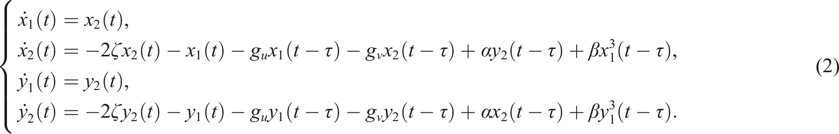
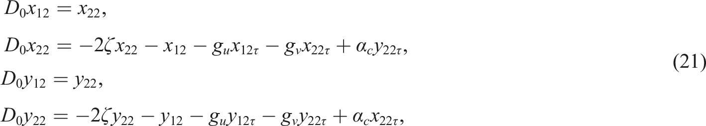
The single degree of freedom active control system with delayed feedback is described⁸; we focus on the study of the double Hopf bifurcation induced by time delay and coupling factor. So this paper is paid to the time delay coupled active control system, which is as follows:

{\begin{cases} {\ddot{x}}_{1} (t) + 2 ζ {\dot{x}}_{1} (t) + x_{1} (t) + g_{u} x_{1} (t - τ) + g_{v} {\dot{x}}_{1} (t - τ) = α {\dot{y}}_{1} (t - τ) + β x_{1}^{3} (t - τ), \\ {\ddot{y}}_{1} (t) + 2 ζ {\dot{y}}_{1} (t) + y_{1} (t) + g_{u} y_{1} (t - τ) + g_{v} {\dot{y}}_{1} (t - τ) = α {\dot{x}}_{1} (t - τ) + β y_{1}^{3} (t - τ), \end{cases}

(1)

where

t^{*} = \sqrt{k / m t}

ζ = c / 2 m \sqrt{m / k}

, g_u = u/k,

g_{v} = v / m \sqrt{m / k}

, and β = a/k. For convenience, let t* = t, x₁(t) and y₁(t) are the displacements of the controlled system, m > 0 is the mass, c and k are damping and the stiffness, respectively, τ is the time delay, u v are feedback strengths, α is the coupling strength, and a is the external excitation factor.

Let ${\dot{x}}_{1} = x_{2}$ and ${\dot{y}}_{1} = y_{2}$ , then system (1) becomes as follows:

{\begin{cases} {\dot{x}}_{1} (t) = x_{2} (t), \\ {\dot{x}}_{2} (t) = - 2 ζ x_{2} (t) - x_{1} (t) - g_{u} x_{1} (t - τ) - g_{v} x_{2} (t - τ) + α y_{2} (t - τ) + β x_{1}^{3} (t - τ), \\ {\dot{y}}_{1} (t) = y_{2} (t), \\ {\dot{y}}_{2} (t) = - 2 ζ y_{2} (t) - y_{1} (t) - g_{u} y_{1} (t - τ) - g_{v} y_{2} (t - τ) + α x_{2} (t - τ) + β y_{1}^{3} (t - τ) . \end{cases}

(2)

System (2) has equilibriums E₀ = (0, 0, 0, 0), $E_{1} = (\sqrt{1 + g_{u} / β}, 0, \sqrt{1 + g_{u} / β}, 0)$ , $E_{2} = (\sqrt{1 + g_{u} / β}, 0, - \sqrt{1 + g_{u} / β}, 0)$ , $E_{3} = (- \sqrt{1 + g_{u} / β}, 0, \sqrt{1 + g_{u} / β}, 0)$ , and $E_{4} = (- \sqrt{1 + g_{u} / β}, 0, - \sqrt{1 + g_{u} / β}, 0)$ . The case of other equilibrium points can be transformed into the case of trivial equilibrium points by coordinate transformation, so here we only consider the stability of the system at trivial equilibrium points. The characteristic equation at zero is

(λ^{2} + 2 ζ λ + (g_{v} + α) λ e^{- λ τ} + g_{u} e^{- λ τ} + 1) (λ^{2} + 2 ζ λ + (g_{v} - α) λ e^{- λ τ} + g_{u} e^{- λ τ} + 1) = 0

(3)

In order to study the distribution of characteristic roots, we first introduce the following lemma,³⁰ which will be used in proving theorems:

Lemma 1

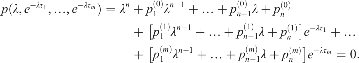
For transcendental equation

\begin{array}{l} p (λ, e^{- λ τ_{1}}, \dots, e^{- λ τ_{m}}) = λ^{n} + p_{1}^{(0)} λ^{n - 1} + \dots + p_{n - 1}^{(0)} λ + p_{n}^{(0)} \\ + [p_{1}^{(1)} λ^{n - 1} + \dots + p_{n - 1}^{(1)} λ + p_{n}^{(1)}] e^{- λ τ_{1}} + \dots \\ + [p_{1}^{(m)} λ^{n - 1} + \dots + p_{n - 1}^{(m)} λ + p_{n}^{(m)}] e^{- λ τ_{m}} = 0 . \end{array}

as (τ₁, τ₂, τ₃, …, τ_m) change, the sum of orders of the zeros of

p (λ, e^{- λ τ_{1}}, \dots, e^{- λ τ_{m}})

in the open right half plane can alter, and only a zero occurs on or passes through the imaginary axis.

Stability switches: Case one

When g_u + 1 ≠ 0, λ = 0 is not the root of equation (3).

Consider

λ^{2} + 2 ζ λ + (g_{v} + α) λ e^{- λ τ} + g_{u} e^{- λ τ} + 1 = 0

(4)

let iω(ω > 0) be a root of equation (4), then separating the real and imaginary parts yields

{\begin{cases} ω^{2} - 1 = (g_{v} + α) ω \sin (ω τ) + g_{u} \cos (ω τ), \\ 2 ζ ω = - (g_{v} + α) ω \cos (ω τ) + g_{u} \sin (ω τ) . \end{cases}

(5)

from equation (5) we obtain

ω^{4} + {(4 ζ^{2} - 2 - (g_{v} + α)}^{2}) ω^{2} + 1 - g_{u}^{2} = 0

Let z = ω², then we have

h (z) = z^{2} + {(4 ζ^{2} - 2 - (g_{v} + α)}^{2}) z + 1 - g_{u}^{2} = 0

(6)

where

△ = {({4 ζ}^{2} - 2 - {(g_{v} + a)}^{2})}^{2} - 4 (1 - g_{u}^{2})

When $1 - g_{u}^{2} > 0$ , △ > 0, $2 + {(g_{v} + α)}^{2} - 4 ζ^{2} > 0$ , equation (6) has two positive roots

z_{\pm} = \frac{2 + {(g_{v} + α)}^{2} - 4 ζ^{2} \pm \sqrt{△}}{2}

then

ω_{\pm} = \sqrt{z_{\pm}} = \sqrt{\frac{2 + {(g_{v} + α)}^{2} - 4 ζ^{2} \pm \sqrt{△}}{2}}

(7)

furthermore, it follows from equation (5) that

\sin (ω τ) = \frac{(ω^{2} - 1) (g_{v} + α) ω + 2 ζ ω g_{u}}{g_{u}^{2} + ω^{2} {(g_{v} + α)}^{2}}

(8)

\cos (ω τ) = \frac{(ω^{2} - 1) g_{u} - 2 ζ ω^{2} (g_{v} + α)}{g_{u}^{2} + ω^{2} {(g_{v} + α)}^{2}}

(9)

by equation (9) we have

{\begin{cases} τ_{\pm}^{(k)} = \frac{1}{ω_{\pm}} (a r c \cos \frac{(ω^{2} - 1) g_{u} - 2 ζ ω^{2} (g_{v} + α)}{g_{u}^{2} + ω^{2} {(g_{v} + α)}^{2}} + 2 k π), k = 0, 1, 2, \dots, \sin ω τ \geq 0, \\ τ_{\pm}^{(k)} = \frac{1}{ω_{\pm}} (2 π - a r c \cos \frac{(ω^{2} - 1) g_{u} - 2 ζ ω^{2} (g_{v} + α)}{g_{u}^{2} + ω^{2} {(g_{v} + α)}^{2}} + 2 k π), k = 0, 1, 2, \dots, \sin ω τ < 0 . \end{cases}

(10)

The transversality condition is verified below, substituting λ into equation (4) and taking the derivative with respect to τ, we get

Re {(\frac{d λ}{d τ})}_{τ = τ_{\pm}^{(k)}}^{- 1} = \frac{2 ω_{\pm}^{2} - 2 - {(g_{v} + α)}^{2} + 4 ζ^{2}}{ω_{\pm}^{2} {(g_{v} + α)}^{2} + g_{u}^{2}} = \frac{h^{'} (z)}{ω_{\pm}^{2} {(g_{v} + α)}^{2} + g_{u}^{2}}

from which we obtain

R e {(\frac{d λ}{d τ})}_{τ = τ_{-}^{(k)}}^{- 1} < 0, R e {(\frac{d λ}{d τ})}_{τ = τ_{+}^{(k)}}^{- 1} > 0

Combined with Lemma 1 and theory of Hopf bifurcation, we can derive the following theorem.

Theorem 1

Suppose that 4ζ + 2g_v > 0, $2 (g_{u} + 1) + {(2 ζ + g_{v})}^{2} - α^{2} > 0$ , (2ζ + g_v)(g_u + 1) > 0, $2 (g_{u} + 1) + {(2 ζ + g_{v})}^{2} - α^{2} > g_{u} + 1$ hold, if $1 - g_{u}^{2} > 0$ , △ > 0, $2 + {(g_{v} + α)}^{2} - 4 ζ^{2} > 0$ ,

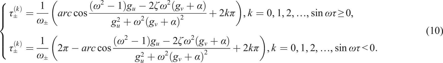
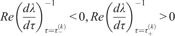
(i) When $τ = τ_{\pm}^{(k)}$ , then the trivial equilibrium of system (1) undergoes a Hopf bifurcation, and there exists n ∈ N, such that $0 < τ_{+}^{(0)} < τ_{-}^{(0)} < τ_{+}^{(1)} < τ_{-}^{(1)} < \dots < τ_{+}^{(n)} < τ_{-}^{(n)} < τ_{+}^{(n + 1)} < τ_{-}^{(n + 1)} < \dots$ , when $τ \in [0, τ_{+}^{(0)}) \cup \cup_{k = 0}^{n} (τ_{-}^{(k)}, τ_{+}^{(k + 1)})$ , E₀ is local asymptotic stable; when $τ \in \cup_{k = 0}^{n} (τ_{+}^{(k)}, τ_{-}^{(k + 1)}) \cup (τ_{+}^{(n + 1)}, \infty)$ , E₀ is unstable.

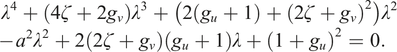
(ii) When $τ_{-}^{(i)} = τ_{+}^{(j)}$ , then system (1) occurs double Hopf bifurcation, where ω_± is given in equation (7) and $τ_{\pm}^{(k)}$ is given in equation (10).Proof: Here we only prove (i), when τ = 0, equation (3) becomes

\begin{array}{l} λ^{4} + (4 ζ + 2 g_{v}) λ^{3} + (2 (g_{u} + 1) + {(2 ζ + g_{v})}^{2}) λ^{2} \\ - a^{2} λ^{2} + 2 (2 ζ + g_{v}) (g_{u} + 1) λ + {(1 + g_{u})}^{2} = 0 . \end{array}

According to Routh–Hurwitz, when 4ζ + 2g_v > 0, $2 (g_{u} + 1) + {(2 ζ + g_{v})}^{2} - α^{2} > 0$ , (2ζ + g_v)(g_u + 1) > 0, $2 (g_{u} + 1) + {(2 ζ + g_{v})}^{2} - α^{2} > g_{u} + 1$ hold, the roots of the above equation have all negative real parts. The trivial equilibrium is local asymptotic stable for any τ.

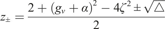
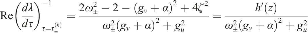
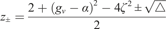
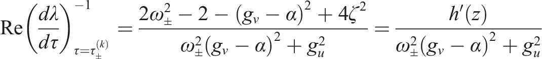
When $1 - g_{u}^{2} > 0$ , △ > 0, $2 + {(g_{v} + α)}^{2} - 4 ζ^{2} > 0$ hold, h(z) has two positive roots, and $R e {(d λ / d τ)}_{τ = τ_{-}^{(k)}}^{- 1} < 0$ , $R e {(d λ / d τ)}_{τ = τ_{+}^{(k)}}^{- 1} > 0$ . Therefore, when $τ \in [0, τ_{+}^{(0)}) \cup \cup_{k = 0}^{n} (τ_{-}^{(k)}, τ_{+}^{(k + 1)})$ , all the roots of equation (4) have negative real parts, and equation (4) has at least one root with positive real part when $τ \in \cup_{k = 0}^{n} (τ_{+}^{(k)}, τ_{-}^{(k + 1)}) \cup (τ_{+}^{(n + 1)}, \infty)$ .

The proof is completed.

Stability switches: Case two

When g_u + 1 ≠ 0, λ = 0 is not the root of equation (3).

Consider

λ^{2} + 2 ζ λ + (g_{v} - α) λ e^{- λ τ} + g_{u} e^{- λ τ} + 1 = 0

(11)

let iω(ω > 0) be a root of equation (11),then separating the real and imaginary parts yields

{\begin{cases} ω^{2} - 1 = (g_{v} - α) ω \sin (ω τ) + g_{u} \cos (ω τ), \\ 2 ζ ω = - (g_{v} - α) ω \cos (ω τ) + g_{u} \sin (ω τ), \end{cases}

(12)

from equation (12), we obtain

ω^{4} + {(4 ζ^{2} - 2 - (g_{v} - α)}^{2}) ω^{2} + 1 - g_{u}^{2} = 0

Let z = ω², then we have

h (z) = z^{2} + {(4 ζ^{2} - 2 - (g_{v} - α)}^{2}) z + 1 - g_{u}^{2} = 0

(13)

where

△ = {({4 ζ}^{2} - 2 - {(g_{v} + a)}^{2})}^{2} - 4 (1 - g_{u}^{2})

When $1 - g_{u}^{2} > 0$ , △ > 0, $2 + {(g_{v} - α)}^{2} - 4 ζ^{2} > 0$ , equation (6) has two positive roots

z_{\pm} = \frac{2 + {(g_{v} - α)}^{2} - 4 ζ^{2} \pm \sqrt{△}}{2}

then

ω_{\pm} = \sqrt{z_{\pm}} = \sqrt{\frac{2 + {(g_{v} - α)}^{2} - 4 ζ^{2} \pm \sqrt{△}}{2}}

(14)

further, it follows from equation (12) that

\sin (ω τ) = \frac{(ω^{2} - 1) (g_{v} - α) ω + 2 ζ ω g_{u}}{g_{u}^{2} + ω^{2} {(g_{v} - α)}^{2}}

(15)

\cos (ω τ) = \frac{(ω^{2} - 1) g_{u} - 2 ζ ω^{2} (g_{v} - α)}{g_{u}^{2} + ω^{2} {(g_{v} - α)}^{2}}

(16)

it follows from equation (16) that

{\begin{cases} τ_{\pm}^{(k)} = \frac{1}{ω_{\pm}} (a r c \cos \frac{(ω^{2} - 1) g_{u} - 2 ζ ω^{2} (g_{v} - α)}{g_{u}^{2} + ω^{2} {(g_{v} - α)}^{2}} + 2 k π), k = 0, 1, 2, \dots, \sin ω τ \geq 0, \\ τ_{\pm}^{(k)} = \frac{1}{ω_{\pm}} (2 π - a r c \cos \frac{(ω^{2} - 1) g_{u} - 2 ζ ω^{2} (g_{v} - α)}{g_{u}^{2} + ω^{2} {(g_{v} - α)}^{2}} + 2 k π), k = 0, 1, 2, \dots, \sin ω τ < 0 . \end{cases}

(17)

Substituting λ into equation (11) and taking the derivative with respect to τ, we can get

Re {(\frac{d λ}{d τ})}_{τ = τ_{\pm}^{(k)}}^{- 1} = \frac{2 ω_{\pm}^{2} - 2 - {(g_{v} - α)}^{2} + 4 ζ^{2}}{ω_{\pm}^{2} {(g_{v} - α)}^{2} + g_{u}^{2}} = \frac{h^{'} (z)}{ω_{\pm}^{2} {(g_{v} - α)}^{2} + g_{u}^{2}}

from which we know

R e {(\frac{d λ}{d τ})}_{τ = τ_{-}^{(k)}}^{- 1} < 0, R e {(\frac{d λ}{d τ})}_{τ = τ_{+}^{(k)}}^{- 1} > 0

which means the transversality condition holds.

Combined with lemma 1 and theory of Hopf bifurcation, the following theorem can be obtained.

Theorem 2

(i) When $τ = τ_{\pm}^{(k)}$ , then the trivial equilibrium of system (1) undergoes a Hopf bifurcation, and there exists n ∈ N, such that $0 < τ_{+}^{(0)} < τ_{-}^{(0)} < τ_{+}^{(1)} < τ_{-}^{(1)} < \dots < τ_{+}^{(n)} < τ_{-}^{(n)} < τ_{+}^{(n + 1)} < τ_{-}^{(n + 1)} < \dots$ , when $τ \in [0, τ_{+}^{(0)}) \cup \cup_{k = 0}^{n} (τ_{-}^{(k)}, τ_{+}^{(k + 1)})$ , E₀ is local asymptotic stable; when $τ \in \cup_{k = 0}^{n} (τ_{+}^{(k)}, τ_{-}^{(k + 1)}) \cup (τ_{+}^{(n + 1)}, \infty)$ , E₀ is unstable.

(ii) When $τ_{-}^{(i)} = τ_{+}^{(j)}$ , then system (1) occurs double Hopf bifurcation, where ω_± is given in equation (14) and $τ_{\pm}^{(k)}$ is given in equation (17).Proof: The proof here is similar to that of the theorem 1, which is deleted here.

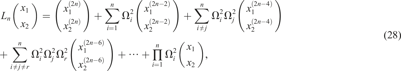
The normal form

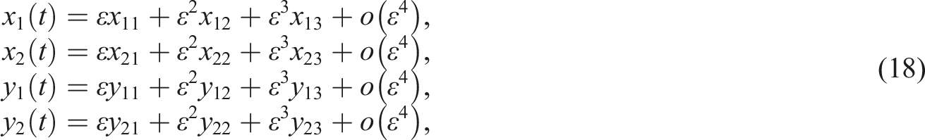
In this section, we first derive the normal form of double Hopf bifurcation by multiple-scale method and then give a bifurcation analysis. We treat the coupling strength α and the time delay τ as two bifurcation parameters. Suppose that system (2) undergoes a double Hopf bifurcation from the trivial equilibrium at the critical point: α = α_c and τ = τ_c. The solution of equation (2) is assumed to take the following form:

\begin{array}{l} x_{1} (t) = ε x_{11} + ε^{2} x_{12} + ε^{3} x_{13} + o (ε^{4}), \\ x_{2} (t) = ε x_{21} + ε^{2} x_{22} + ε^{3} x_{23} + o (ε^{4}), \\ y_{1} (t) = ε y_{11} + ε^{2} y_{12} + ε^{3} y_{13} + o (ε^{4}), \\ y_{2} (t) = ε y_{21} + ε^{2} y_{22} + ε^{3} y_{23} + o (ε^{4}), \end{array}

(18)

where x_ij = x_ij(T₀, T₂), T₀ = t, T₂ = ɛ²t, and 0 < ɛ ≪ 1.

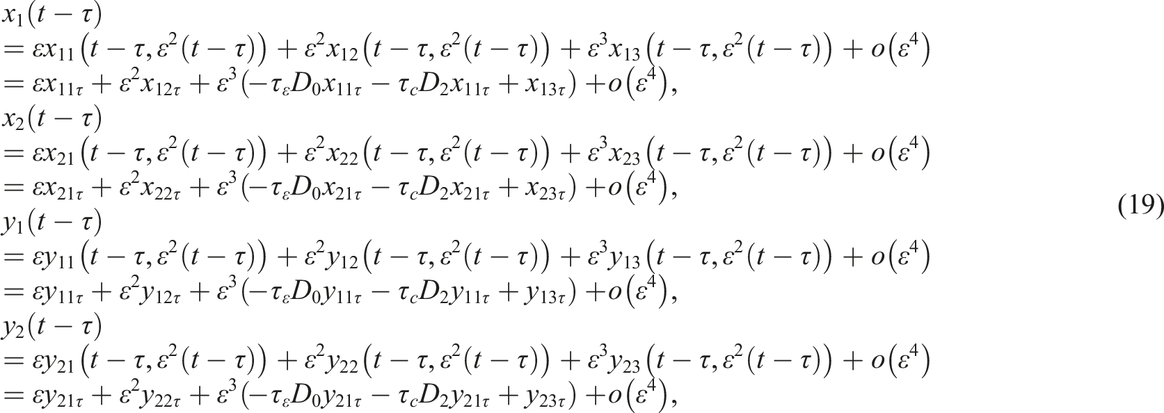
We set perturbations as α = α_c + ɛ²α_ɛ, τ = τ_c + ɛ²τ_ɛ. To deal with the delayed terms of equation (2), we expand

\begin{array}{l} x_{1} (t - τ) \\ = ε x_{11} (t - τ, ε^{2} (t - τ)) + ε^{2} x_{12} (t - τ, ε^{2} (t - τ)) + ε^{3} x_{13} (t - τ, ε^{2} (t - τ)) + o (ε^{4}) \\ = ε x_{11 τ} + ε^{2} x_{12 τ} + ε^{3} (- τ_{ε} D_{0} x_{11 τ} - τ_{c} D_{2} x_{11 τ} + x_{13 τ}) + o (ε^{4}), \\ x_{2} (t - τ) \\ = ε x_{21} (t - τ, ε^{2} (t - τ)) + ε^{2} x_{22} (t - τ, ε^{2} (t - τ)) + ε^{3} x_{23} (t - τ, ε^{2} (t - τ)) + o (ε^{4}) \\ = ε x_{21 τ} + ε^{2} x_{22 τ} + ε^{3} (- τ_{ε} D_{0} x_{21 τ} - τ_{c} D_{2} x_{21 τ} + x_{23 τ}) + o (ε^{4}), \\ y_{1} (t - τ) \\ = ε y_{11} (t - τ, ε^{2} (t - τ)) + ε^{2} y_{12} (t - τ, ε^{2} (t - τ)) + ε^{3} y_{13} (t - τ, ε^{2} (t - τ)) + o (ε^{4}) \\ = ε y_{11 τ} + ε^{2} y_{12 τ} + ε^{3} (- τ_{ε} D_{0} y_{11 τ} - τ_{c} D_{2} y_{11 τ} + y_{13 τ}) + o (ε^{4}), \\ y_{2} (t - τ) \\ = ε y_{21} (t - τ, ε^{2} (t - τ)) + ε^{2} y_{22} (t - τ, ε^{2} (t - τ)) + ε^{3} y_{23} (t - τ, ε^{2} (t - τ)) + o (ε^{4}) \\ = ε y_{21 τ} + ε^{2} y_{22 τ} + ε^{3} (- τ_{ε} D_{0} y_{21 τ} - τ_{c} D_{2} y_{21 τ} + y_{23 τ}) + o (ε^{4}), \end{array}

(19)

where x_ijτ = x_ij(T₀ − τ_c, T₂), y_ijτ = y_ij(T₀ − τ_c, T₂), D₀ = ∂/∂T₀, and D₂ = ∂/∂T₂.

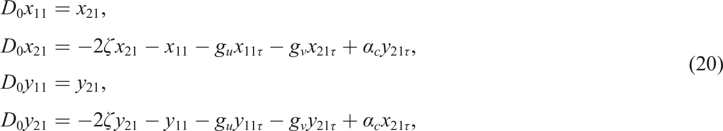
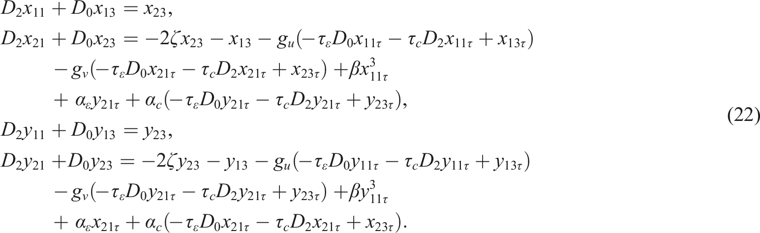
Then, substituting solution equation (19) into equation (2) and balancing the coefficients ɛ, ɛ², and ɛ³, we can getɛ:

\begin{array}{l} \begin{array}{l} D_{0} x_{11} = x_{21}, \\ D_{0} x_{21} = - 2 ζ x_{21} - x_{11} - g_{u} x_{11 τ} - g_{v} x_{21 τ} + α_{c} y_{21 τ}, \end{array} \\ \begin{array}{l} D_{0} y_{11} = y_{21}, \\ D_{0} y_{21} = - 2 ζ y_{21} - y_{11} - g_{u} y_{11 τ} - g_{v} y_{21 τ} + α_{c} x_{21 τ}, \end{array} \end{array}

(20)

ɛ²:

\begin{array}{l} \begin{array}{l} D_{0} x_{12} = x_{22}, \\ D_{0} x_{22} = - 2 ζ x_{22} - x_{12} - g_{u} x_{12 τ} - g_{v} x_{22 τ} + α_{c} y_{22 τ}, \end{array} \\ D_{0} y_{12} = y_{22}, \\ D_{0} y_{22} = - 2 ζ y_{22} - y_{12} - g_{u} y_{12 τ} - g_{v} y_{22 τ} + α_{c} x_{22 τ}, \end{array}

(21)

ɛ³:

\begin{array}{l} D_{2} x_{11} + D_{0} x_{13} = x_{23}, \\ D_{2} x_{21} + D_{0} x_{23} = - 2 ζ x_{23} - x_{13} - g_{u} (- τ_{ε} D_{0} x_{11 τ} - τ_{c} D_{2} x_{11 τ} + x_{13 τ}) \\ - g_{v} (- τ_{ε} D_{0} x_{21 τ} - τ_{c} D_{2} x_{21 τ} + x_{23 τ}) + β x_{11 τ}^{3} \\ + α_{ε} y_{21 τ} + α_{c} (- τ_{ε} D_{0} y_{21 τ} - τ_{c} D_{2} y_{21 τ} + y_{23 τ}), \\ D_{2} y_{11} + D_{0} y_{13} = y_{23}, \\ D_{2} y_{21} + D_{0} y_{23} = - 2 ζ y_{23} - y_{13} - g_{u} (- τ_{ε} D_{0} y_{11 τ} - τ_{c} D_{2} y_{11 τ} + y_{13 τ}) \\ - g_{v} (- τ_{ε} D_{0} y_{21 τ} - τ_{c} D_{2} y_{21 τ} + y_{23 τ}) + β y_{11 τ}^{3} \\ + α_{ε} x_{21 τ} + α_{c} (- τ_{ε} D_{0} x_{21 τ} - τ_{c} D_{2} x_{21 τ} + x_{23 τ}) . \end{array}

(22)

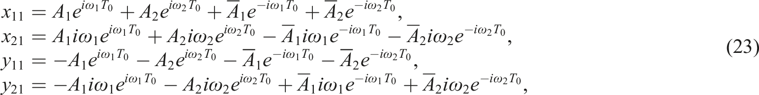
Suppose the solution of equation (20) can be expressed in the form of

\begin{array}{l} x_{11} = A_{1} e^{i ω_{1} T_{0}} + A_{2} e^{i ω_{2} T_{0}} + {\bar{A}}_{1} e^{- i ω_{1} T_{0}} + {\bar{A}}_{2} e^{- i ω_{2} T_{0}}, \\ x_{21} = A_{1} i ω_{1} e^{i ω_{1} T_{0}} + A_{2} i ω_{2} e^{i ω_{2} T_{0}} - {\bar{A}}_{1} i ω_{1} e^{- i ω_{1} T_{0}} - {\bar{A}}_{2} i ω_{2} e^{- i ω_{2} T_{0}}, \\ y_{11} = - A_{1} e^{i ω_{1} T_{0}} - A_{2} e^{i ω_{2} T_{0}} - {\bar{A}}_{1} e^{- i ω_{1} T_{0}} - {\bar{A}}_{2} e^{- i ω_{2} T_{0}}, \\ y_{21} = - A_{1} i ω_{1} e^{i ω_{1} T_{0}} - A_{2} i ω_{2} e^{i ω_{2} T_{0}} + {\bar{A}}_{1} i ω_{1} e^{- i ω_{1} T_{0}} + {\bar{A}}_{2} i ω_{2} e^{- i ω_{2} T_{0}}, \end{array}

(23)

where A_j, j = 1, 2 are complex constants with respect to T₂.

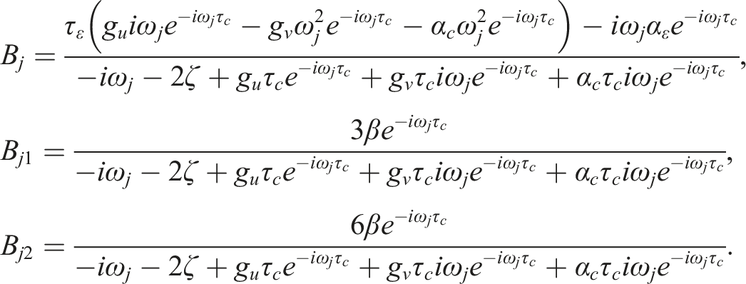
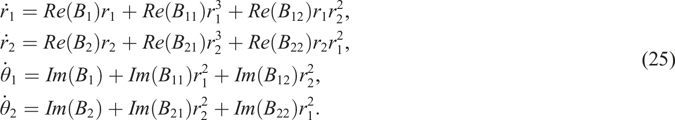
Substituting equation (23) into equation (21) and equation (22), eliminate the secular term to obtain the complex amplitude equation:

\begin{array}{l} {\dot{A}}_{1} = B_{1} A_{1} + B_{11} A_{1}^{2} {\bar{A}}_{1} + B_{12} A_{1} A_{2} {\bar{A}}_{2}, \\ {\dot{A}}_{2} = B_{2} A_{2} + B_{21} A_{2}^{2} {\bar{A}}_{2} + B_{22} A_{2} A_{1} {\bar{A}}_{1}, \end{array}

(24)

where the complex coefficients are expressed as follow:

\begin{array}{l} B_{j} = \frac{τ_{ε} (g_{u} i ω_{j} e^{- i ω_{j} τ_{c}} - g_{v} ω_{j}^{2} e^{- i ω_{j} τ_{c}} - α_{c} ω_{j}^{2} e^{- i ω_{j} τ_{c}}) - i ω_{j} α_{ε} e^{- i ω_{j} τ_{c}}}{- i ω_{j} - 2 ζ + g_{u} τ_{c} e^{- i ω_{j} τ_{c}} + g_{v} τ_{c} i ω_{j} e^{- i ω_{j} τ_{c}} + α_{c} τ_{c} i ω_{j} e^{- i ω_{j} τ_{c}}}, \\ B_{j 1} = \frac{3 β e^{- i ω_{j} τ_{c}}}{- i ω_{j} - 2 ζ + g_{u} τ_{c} e^{- i ω_{j} τ_{c}} + g_{v} τ_{c} i ω_{j} e^{- i ω_{j} τ_{c}} + α_{c} τ_{c} i ω_{j} e^{- i ω_{j} τ_{c}}}, \\ B_{j 2} = \frac{6 β e^{- i ω_{j} τ_{c}}}{- i ω_{j} - 2 ζ + g_{u} τ_{c} e^{- i ω_{j} τ_{c}} + g_{v} τ_{c} i ω_{j} e^{- i ω_{j} τ_{c}} + α_{c} τ_{c} i ω_{j} e^{- i ω_{j} τ_{c}}} . \end{array}

let

A_{1} = r_{1} e^{i θ_{1}}

and

A_{2} = r_{2} e^{i θ_{2}}

, equation (24) becomes

\begin{array}{l} {\dot{r}}_{1} = R e (B_{1}) r_{1} + R e (B_{11}) r_{1}^{3} + R e (B_{12}) r_{1} r_{2}^{2}, \\ {\dot{r}}_{2} = R e (B_{2}) r_{2} + R e (B_{21}) r_{2}^{3} + R e (B_{22}) r_{2} r_{1}^{2}, \\ {\dot{θ}}_{1} = I m (B_{1}) + I m (B_{11}) r_{1}^{2} + I m (B_{12}) r_{2}^{2}, \\ {\dot{θ}}_{2} = I m (B_{2}) + I m (B_{21}) r_{2}^{2} + I m (B_{22}) r_{1}^{2} . \end{array}

(25)

Now consider the normal form equations:

\begin{array}{l} {\dot{r}}_{1} = R e (B_{1}) r_{1} + R e (B_{11}) r_{1}^{3} + R e (B_{12}) r_{1} r_{2}^{2}, \\ {\dot{r}}_{2} = R e (B_{2}) r_{2} + R e (B_{21}) r_{2}^{3} + R e (B_{22}) r_{2} r_{1}^{2} . \end{array}

(26)

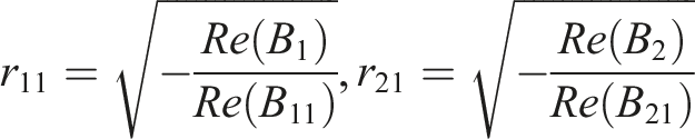
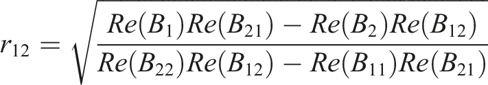
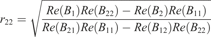
According to the normal form equations, we can obtain all possible equilibrium points

M_{0} = (0, 0), M_{1} = (r_{11}, 0), M_{2} = (0, r_{21}), M_{3} = (r_{12}, r_{22})

where

r_{11} = \sqrt{- \frac{R e (B_{1})}{R e (B_{11})}}, r_{21} = \sqrt{- \frac{R e (B_{2})}{R e (B_{21})}}

r_{12} = \sqrt{\frac{R e (B_{1}) R e (B_{21}) - R e (B_{2}) R e (B_{12})}{R e (B_{22}) R e (B_{12}) - R e (B_{11}) R e (B_{21})}}

r_{22} = \sqrt{\frac{R e (B_{1}) R e (B_{22}) - R e (B_{2}) R e (B_{11})}{R e (B_{21}) R e (B_{11}) - R e (B_{12}) R e (B_{22})}}

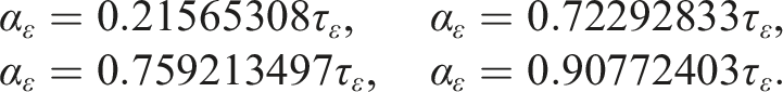
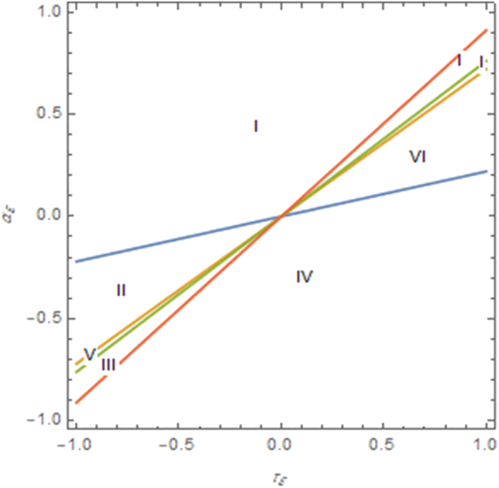
The existence and stability of the above possible equilibrium points is dependent on α_ɛ, τ_ɛ. Here we consider the case of 3:5 resonance in the first case. Let g_u = 0, $g_{v} = \sqrt{15} / 5$ , ζ = 0, β = 0.1, and $α = - \sqrt{15} / 15$ , we obtain $ω_{+} = \sqrt{15} / 3$ , $τ_{+}^{(1)} = \sqrt{15} π / 2$ , $ω_{-} = \sqrt{15} / 5$ , and $τ_{-}^{(0)} = \sqrt{15} π / 2$ .

The critical bifurcation line can also be obtained as follows:

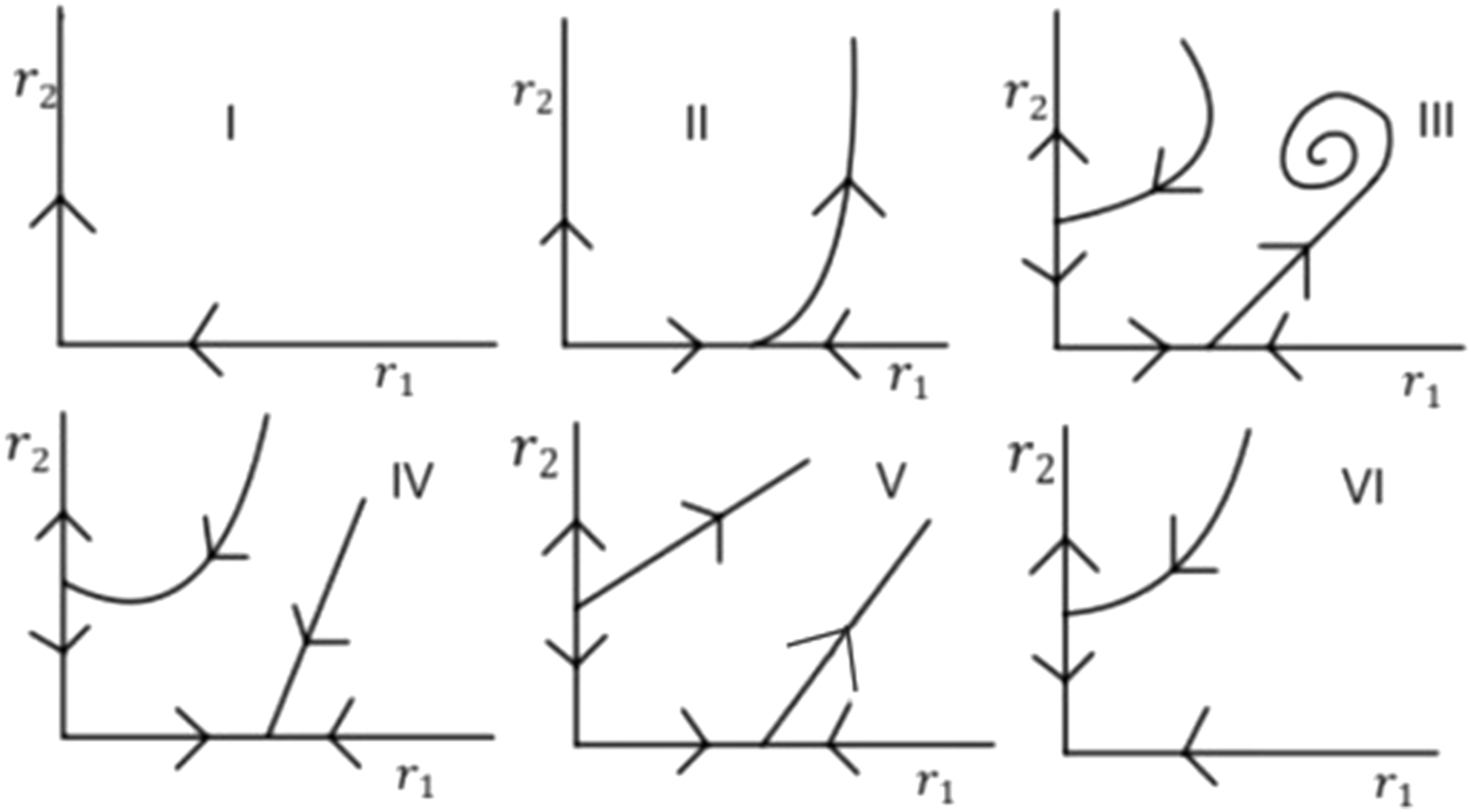
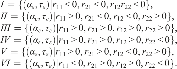
\begin{array}{l} α_{ε} = 0.21565308 τ_{ε}, & α_{ε} = 0.72292833 τ_{ε}, \\ α_{ε} = 0.759213497 τ_{ε}, & α_{ε} = 0.90772403 τ_{ε} . \end{array}

the critical bifurcation line divides the parameter region into six blocks as shown in Figure 1 and 2:

\begin{array}{l} I = {(α_{ε}, τ_{ε}) | r_{11} < 0, r_{21} < 0, r_{12} r_{22} < 0}, \\ I I = {(α_{ε}, τ_{ε}) | r_{11} > 0, r_{21} < 0, r_{12} < 0, r_{22} > 0}, \\ I I I = {(α_{ε}, τ_{ε}) | r_{11} > 0, r_{21} > 0, r_{12} > 0, r_{22} > 0}, \\ I V = {(α_{ε}, τ_{ε}) | r_{11} > 0, r_{21} > 0, r_{12} > 0, r_{22} < 0}, \\ V = {(α_{ε}, τ_{ε}) | r_{11} > 0, r_{21} > 0, r_{12} < 0, r_{22} > 0}, \\ V I = {(α_{ε}, τ_{ε}) | r_{11} < 0, r_{21} > 0, r_{12} > 0, r_{22} < 0} . \end{array}

Figure 1.

Critical bifurcation lines in the (α_ɛ, τ_ɛ) parameter plane around the 3:5 weakly resonant double Hopf bifurcation point (α_c, τ_c).

Figure 2.

Classification of intrinsic dynamic behavior around the 3:5 weakly resonant double Hopf bifurcation point (α_c, τ_c).

When the parameter is taken in region I, the amplitude equation has only one equilibrium point M₀ = (0, 0), which is a saddle.

When the parameter is taken in region II, the amplitude equation has two equilibrium points M₀ = (0, 0) and M₁ = (r₁₁, 0), and equilibrium point M₀ is unstable while M₁ is a saddle. Correspondingly, there exists an unstable periodic solution.

In region III, there are four equilibrium points: M₀ = (0, 0), M₁ = (r₁₁, 0), M₂ = (0, r₂₁), and M₃ = (r₁₂, r₂₂). The equilibrium point M₀ becomes a saddle from an unstable equilibrium point, M₁ becomes a saddle, M₂ is a saddle, and M₃ is stable. Correspondingly, the original system adds an unstable periodic motion and a stable quasiperiodic motion.

With (α_ɛ, τ_ɛ) changing into region IV, the equilibrium point M₃ disappears and there exist three equilibrium points, M₀ = (0, 0), M₁ = (r₁₁, 0), and M₂ = (0, r₂₁), the equilibrium point M₀ is a saddle and M₁ becomes a stable point which is corresponded to a stable periodic motion of the original system, and the quasi-periodic motion of the original system disappears.

While (α_ɛ, τ_ɛ) enters into region V, the amplitude equation has three equilibrium points: M₀ = (0, 0), M₁ = (r₁₁, 0), M₂ = (0, r₂₁). The equilibrium points M₀ and M₁ are saddles, M₂ is unstable, and M₁ periodic motion of the original system changes stable to unstable.

When the parameter is taken in region VI, there exist two equilibrium points: M₀ = (0, 0), M₂ = (0, r₂₁). The equilibrium point M₀ is stable and M₂ is a saddle, and the periodic solution of the corresponding original system vanishes.

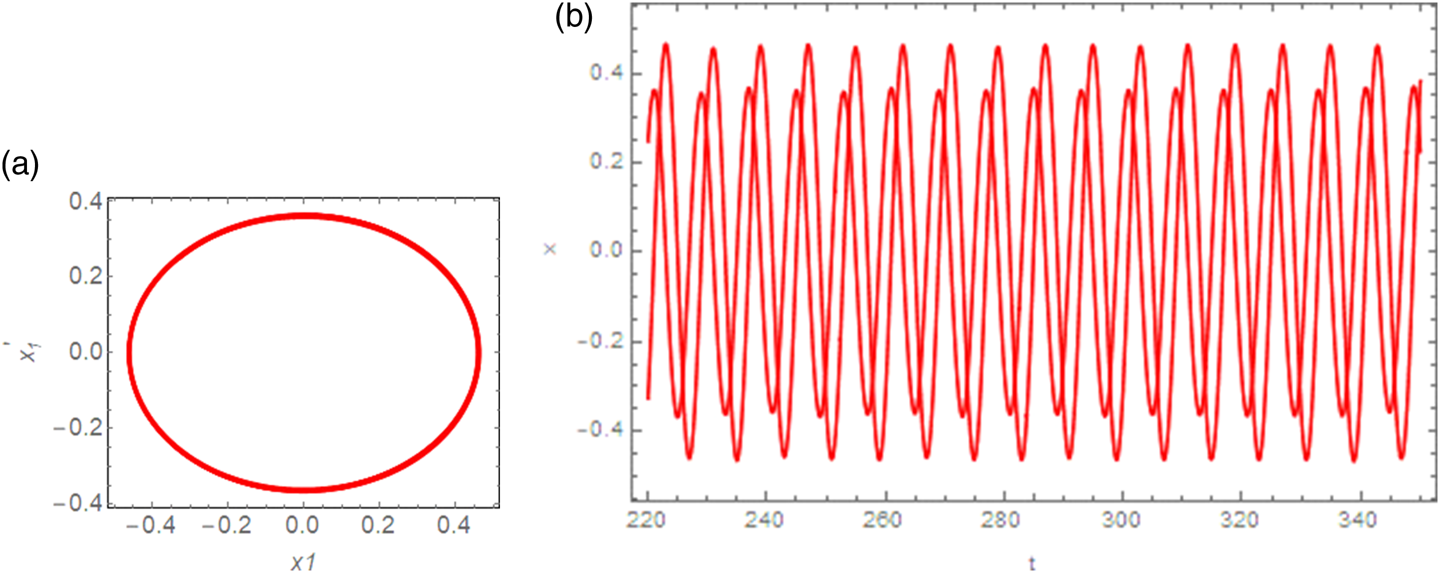
Based on the analysis above, taking the parameters falling in region IV, that is, α = −0.258 and τ = 100.08, the obtained phase portrait and time history are shown in Figure 3:

Figure 3.

Period solution of the time delay coupled active control system when g_u = 0, $g_{v} = \sqrt{15} / 5$ , ζ = 0, β = 0.1, α = −0.258, and τ = 100.08: (a) phase portrait and (b) time history.

When the parameter falls in region III, that is,α = −0.2902 and τ = 6.043668, we obtain Figure 4:

Figure 4.

Quasi period solution of the time delay coupled active control system when g_u = 0, $g_{v} = \sqrt{15} / 5$ , ζ = 0, β = 0.1, α = −0.2902, and τ = 6.043668: (a) phase portrait and (b) time history.

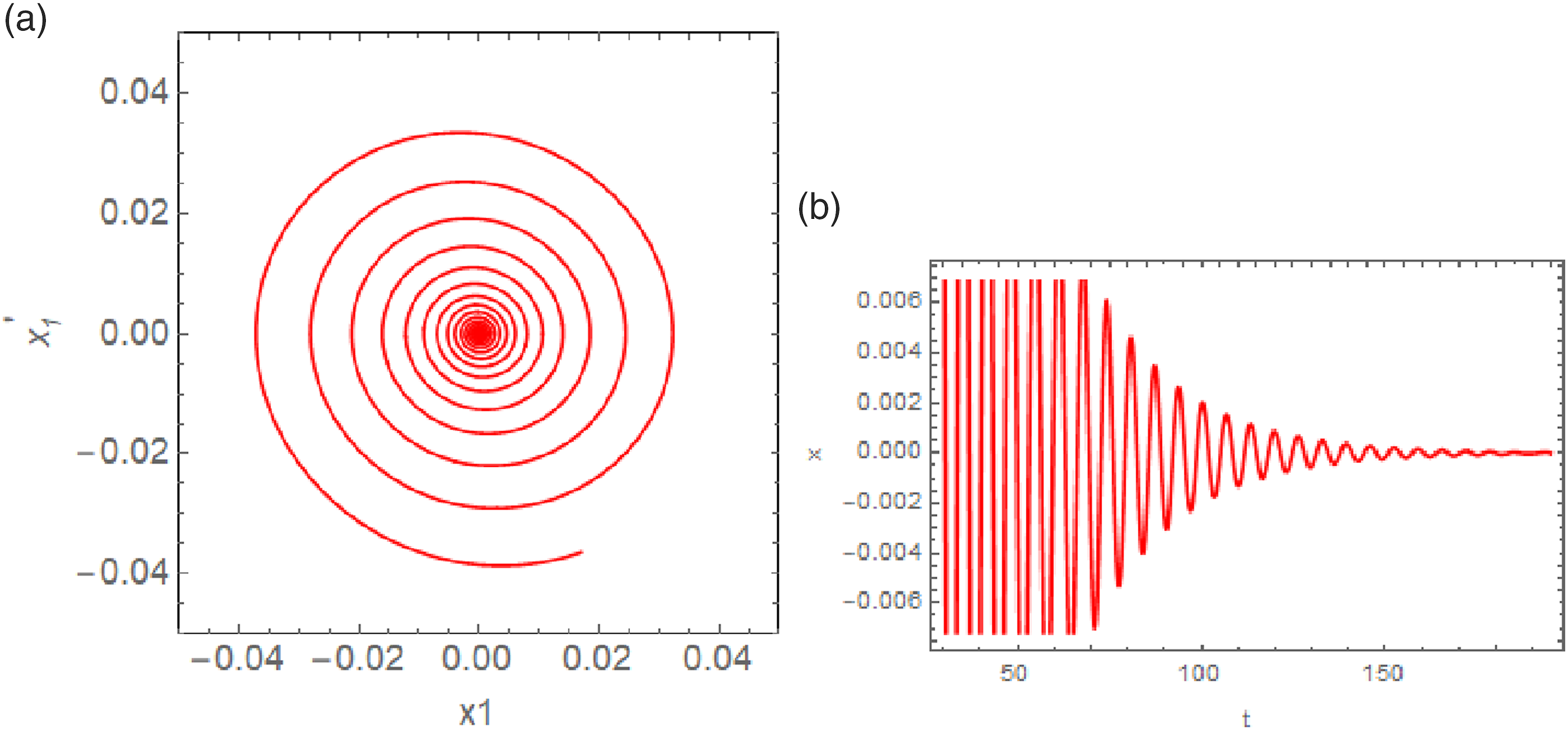
When the parameter is taken in region VI, that is, α = 0.85 and τ = 9.083668, we can obtain Figure 5:

Figure 5.

Stable point of the time delay coupled active control system when g_u = 0, $g_{v} = \sqrt{15} / 5$ , ζ = 0, β = 0.1, α = 0.85, and τ = 9.083668: (a) phase portrait and (b) time history.

From figures above, we can see that the results of the numerical simulation match our theoretical analysis.

Multi-frequency Homotopy Analysis Method

First, we consider the following two-degree-of-freedom system:

\begin{array}{l} x_{1}^{″} + c x_{1}^{'} + F_{1} (x_{1}, x_{2}) = f_{1} \cos Ω t, \\ x_{2}^{″} + c x_{2}^{'} + F_{2} (x_{1}, x_{2}) = f_{2} \cos Ω t, \end{array}

(27)

where x₁(t) and x₂(t) are unknown real functions, F₁(x₁, x₂) and F₂(x₁, x₂) are coupling functions, f₁ and f₂ are amplitudes of excitation, Ω is the frequency of the parametric excitation, and c is a known physical parameter.

According to the MFHAM, we construct the n-order auxiliary linear differential operator as follows:

\begin{array}{l} L_{n} (\begin{array}{l} x_{1} \\ x_{2} \end{array}) = (\begin{array}{l} x_{1}^{(2 n)} \\ x_{2}^{(2 n)} \end{array}) + \sum_{i = 1}^{n} Ω_{i}^{2} (\begin{array}{l} x_{1}^{(2 n - 2)} \\ x_{2}^{(2 n - 2)} \end{array}) + \sum_{i \neq j}^{n} Ω_{i}^{2} Ω_{j}^{2} (\begin{array}{l} x_{1}^{(2 n - 4)} \\ x_{2}^{(2 n - 4)} \end{array}) \\ + \sum_{i \neq j \neq r}^{n} Ω_{i}^{2} Ω_{j}^{2} Ω_{r}^{2} (\begin{array}{l} x_{1}^{(2 n - 6)} \\ x_{2}^{(2 n - 6)} \end{array}) + \dots + \prod_{i = 1}^{n} Ω_{i}^{2} (\begin{array}{l} x_{1} \\ x_{2} \end{array}), \end{array}

(28)

where Ω_i(i = 1, 2, …, n) are fundamental frequencies.

The characteristic polynomial of equation (28) is

P (λ) = \prod_{r = 1}^{n} (λ + r Ω i) (λ - r Ω i)

(29)

Because the considered frequencies multiplied by the imaginary unit i are roots of the characteristic polynomial in equation (29), any sinusoidal terms on the right-hand side of the differential operator L_n(x) with the considered frequencies will pose a secular term and hence need to be eliminated.

When the solutions of nonlinear equations are expected to contain the constant term, the auxiliary linear operator in equation (28) can be modified as follows.

\begin{array}{l} L_{n + 1} (\begin{array}{l} x_{1} \\ x_{2} \end{array}) = (\begin{array}{l} x_{1}^{(2 n + 1)} \\ x_{2}^{(2 n + 1)} \end{array}) + \sum_{i = 1}^{n} Ω_{i}^{2} (\begin{array}{l} x_{1}^{(2 n - 1)} \\ x_{2}^{(2 n - 1)} \end{array}) + \sum_{i \neq j}^{n} Ω_{i}^{2} Ω_{j}^{2} (\begin{array}{l} x_{1}^{(2 n - 3)} \\ x_{2}^{(2 n - 3)} \end{array}) \\ + \sum_{i \neq j \neq r}^{n} Ω_{i}^{2} Ω_{j}^{2} Ω_{r}^{2} (\begin{array}{l} x_{1}^{(2 n - 5)} \\ x_{2}^{(2 n - 5)} \end{array}) + \dots + \prod_{i = 1}^{n} Ω_{i}^{2} (\begin{array}{l} x_{1}^{'} \\ x_{2}^{'} \end{array}) . \end{array}

(30)

We construct the following homotopy:

(1 - q) L_{n + 1} (\begin{array}{l} x_{1} - g_{1, 0} (t) \\ x_{2} - g_{2, 0} (t) \end{array}) - q ℏ N (\begin{array}{l} x_{1} \\ x_{2} \end{array}) = 0

(31)

where q∈[0,1] is the embedding variable, g_i,0(t)(i=1,2) are the initial solutions of x_i(t)(i=1,2), respectively, and ℏ is the auxiliary parameter.

Assuming that the power series solution of equation (31) is

x_{i} = x_{i, 0} + q x_{i, 1} + q^{2} x_{i, 2} + \dots (i = 1, 2)

(32)

Substituting equation (32) into equation (31), and then eliminating the same term of q, we can get

q^{0} : L_{n + 1} (\begin{array}{l} x_{1, 0} - g_{1, 0} (t) \\ x_{2, 0} - g_{2, 0} (t) \end{array}) = 0

(33)

q^{1} : L_{n + 1} (\begin{array}{l} x_{1, 1} - g_{1, 0} (t) \\ x_{2, 1} - g_{2, 0} (t) \end{array}) = L_{n + 1} (\begin{array}{l} x_{1, 0} - g_{1, 0} (t) \\ x_{2, 0} - g_{2, 0} (t) \end{array}) + ℏ N (\begin{array}{l} x_{1, 0} \\ x_{2, 0} \end{array})

(34)

q^{2} : L_{n + 1} (\begin{array}{l} x_{1, 2} - g_{1, 0} (t) \\ x_{2, 2} - g_{2, 0} (t) \end{array}) = L_{n + 1} (\begin{array}{l} x_{1, 1} - g_{1, 0} (t) \\ x_{2, 1} - g_{2, 0} (t) \end{array}) + {ℏ \frac{\partial N (\begin{array}{l} x_{1} \\ x_{2} \end{array})}{\partial q} |}_{q = 0}

(35)

let the solution to equation (33) be

x_{i, 0} (t) = g_{i, 0} (t) + A_{0} + \sum_{l = 1} A_{l} \sin (Ω_{l} t + ϕ_{l})

(36)

where A₀, A_l, ϕ_l(l = 1, 2, 3, …, n) are constants.

Firstly, substituting equation (33) and equation (36) into equation (34), and eliminating the secular terms, we obtain $L_{n + 1} (\begin{array}{l} x_{1} \\ x_{2} \end{array})$ . Secondly, substituting $L_{n + 1} (\begin{array}{l} x_{1} \\ x_{2} \end{array})$ into equations (28) or (30), then x_i(t)(i=1,2) can be obtained. Finally, we can get the value of A₀, A_l, ϕ_l(l = 1, 2, 3, …, n) by solving the equations consisting of secular terms.

In a similar way, x_i,r(t)(i=1,2) can be determined one by one. Then the solution of equation (31) is

x_{i} (t) = \lim_{q \to 1} x_{i} (t, q) = x_{i, 0} (t) + x_{i, 1} (t) + x_{i, 2} (t) + \dots

(37)

Analyzing the time delay coupled active control system with MFHAM

We consider the time delay coupled active control system by MFHAM

{\begin{cases} {\ddot{x}}_{1} (t) + 2 ζ {\dot{x}}_{1} (t) + x_{1} (t) + g_{u} x_{1} (t - τ) + g_{v} {\dot{x}}_{1} (t - τ) = α {\dot{y}}_{1} (t - τ) + β x_{1}^{3} (t - τ), \\ {\ddot{y}}_{1} (t) + 2 ζ {\dot{y}}_{1} (t) + y_{1} (t) + g_{u} y_{1} (t - τ) + g_{v} {\dot{y}}_{1} (t - τ) = α {\dot{x}}_{1} (t - τ) + β y_{1}^{3} (t - τ) . \end{cases}

For a single period, the characteristic polynomial is

P (λ) = λ \prod_{r = 1}^{3} (λ + r Ω i) (λ - r Ω i)

(38)

The corresponding auxiliary linear differential operator is

L_{4} (\begin{array}{l} x_{1} \\ y_{1} \end{array}) = (\begin{array}{l} x_{1}^{(7)} \\ y_{1}^{(7)} \end{array}) + 14 Ω^{2} (\begin{array}{l} x_{1}^{(5)} \\ y_{1}^{(5)} \end{array}) + 49 Ω^{4} (\begin{array}{l} x_{1}^{(3)} \\ y_{1}^{(3)} \end{array}) + 36 Ω^{6} (\begin{array}{l} x_{1}^{'} \\ y_{1}^{'} \end{array})

(39)

then, we construct the homotopy expression

\begin{array}{l} Γ (\begin{array}{l} x_{1} & q \\ y_{1} & q \end{array}) = L_{4} (\begin{array}{l} x_{1} \\ y_{1} \end{array}) - q L_{4} (\begin{array}{l} x_{1} \\ y_{1} \end{array}) \\ - q ℏ (\begin{array}{l} {\ddot{x}}_{1} (t) + 2 ζ {\dot{x}}_{1} (t) + x_{1} (t) + g_{u} x_{1} (t - τ) + g_{v} {\dot{x}}_{1} (t - τ) - α {\dot{y}}_{1} (t - τ) - β x_{1}^{3} (t - τ) \\ {\ddot{y}}_{1} (t) + 2 ζ {\dot{y}}_{1} (t) + y_{1} (t) + g_{u} y_{1} (t - τ) + g_{v} {\dot{y}}_{1} (t - τ) - α {\dot{x}}_{1} (t - τ) - β y_{1}^{3} (t - τ) \end{array}), \end{array}

(40)

where ℏ is the auxiliary parameter and q∈[0,1] is the embedding variable.

Suppose the solution to equation (1) is

\begin{array}{l} x_{1} = x_{1, 0} + q x_{1, 1} + q^{2} x_{1, 2} + \dots, \\ y_{1} = x_{1, 0} + q y_{1, 1} + q^{2} y_{1, 2} + \dots . \end{array}

(41)

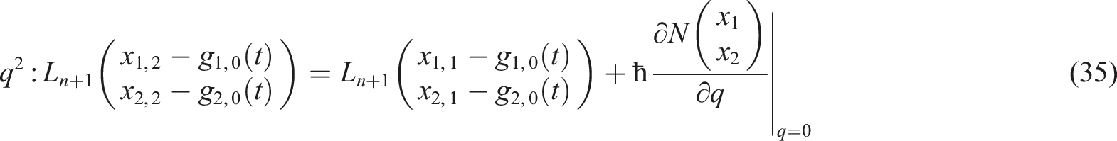
Substituting equation (41) into equation (40) and eliminating the same power terms of q, we can get

q^{0} : L_{4} (\begin{array}{l} x_{1, 0} \\ y_{1, 0} \end{array}) = 0

(42)

\begin{array}{l} q^{1} : L_{4} (\begin{array}{l} x_{1, 1} \\ y_{1, 1} \end{array}) = L_{4} (\begin{array}{l} x_{1, 0} \\ y_{1, 0} \end{array}) \\ + ℏ (\begin{array}{l} {\ddot{x}}_{1, 0} (t) + 2 ζ {\dot{x}}_{1, 0} (t) + x_{1, 0} (t) + g_{u} x_{1, 0} (t - τ) + g_{v} {\dot{x}}_{1, 0} (t - τ) - α {\dot{y}}_{1, 0} (t - τ) \\ {\ddot{y}}_{1, 0} (t) + 2 ζ {\dot{y}}_{1, 0} (t) + y_{1, 0} (t) + g_{u} y_{1, 0} (t - τ) + g_{v} {\dot{y}}_{1, 0} (t - τ) - α {\dot{x}}_{1, 0} (t - τ) \end{array}) . \\ + ℏ (\begin{array}{l} - β x_{1, 0}^{3} (t - τ) \\ - β y_{1, 0}^{3} (t - τ) \end{array}) . \end{array}

(43)

Assuming that solution to equation (42) can be expressed by

\begin{array}{l} x_{1, 0} = a_{1} + b_{1} \cos (Ω t + ϕ_{1}) + b_{2} \cos (2 Ω t + ϕ_{2}) + b_{3} \cos (3 Ω t + ϕ_{3}), \\ y_{1, 0} = a_{2} + d_{1} \cos (Ω t + γ_{1}) + d_{2} \cos (2 Ω t + γ_{2}) + d_{3} \cos (3 Ω t + γ_{3}), \end{array}

(44)

where a₁, a₂, b_i, d_i, ϕ_i, γ_i(i = 1, 2, 3) are unknown parameters.

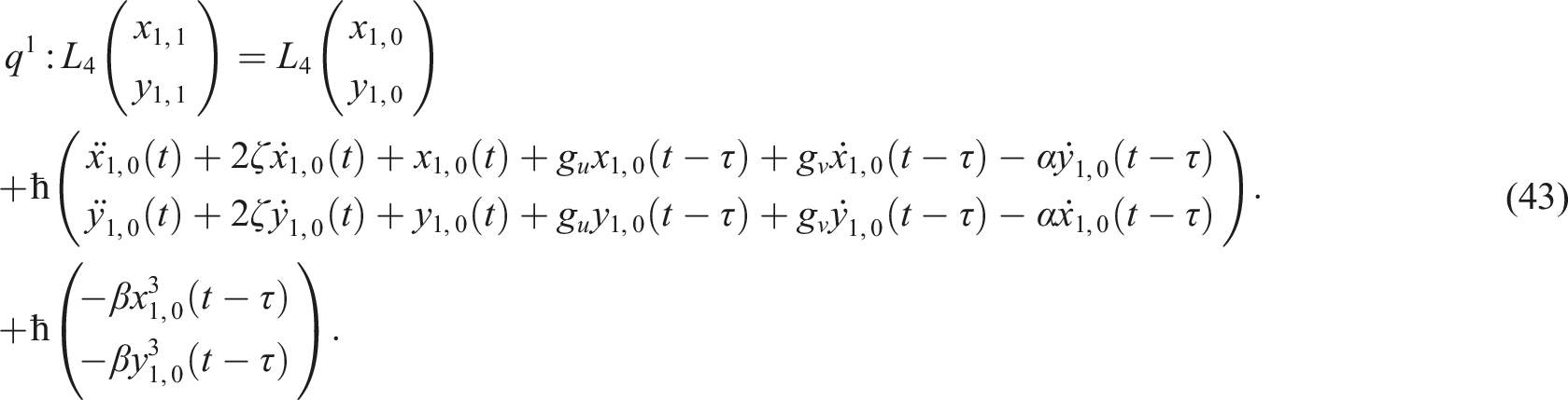
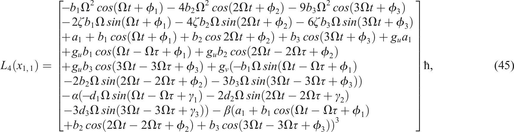
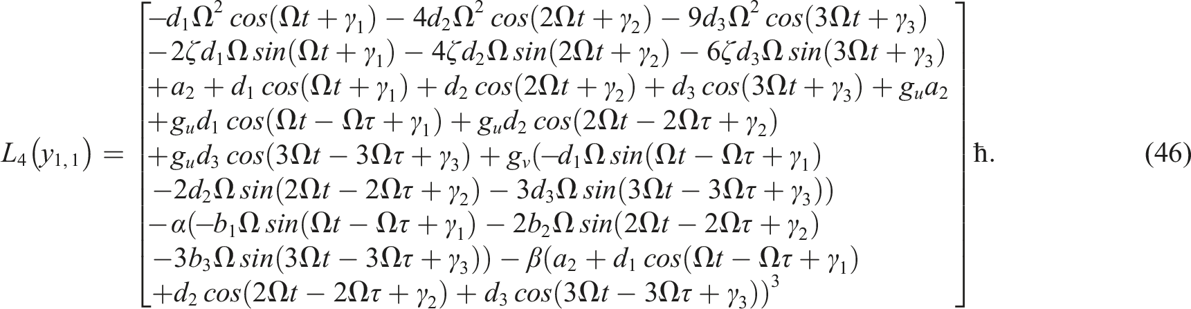
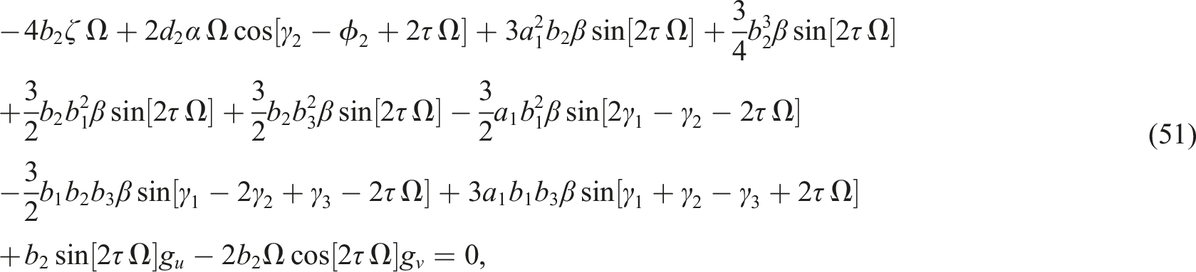
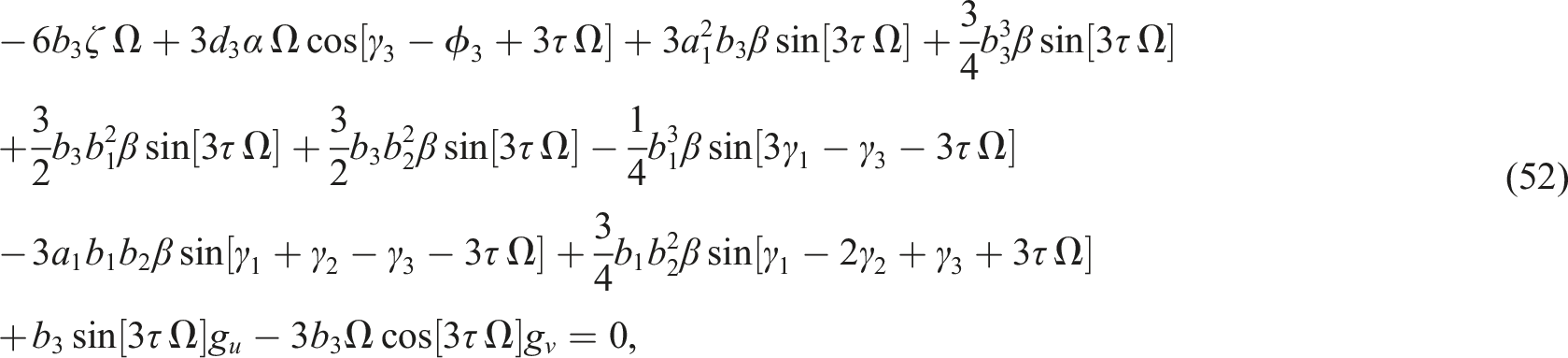
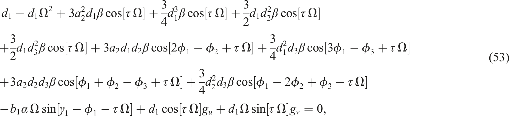
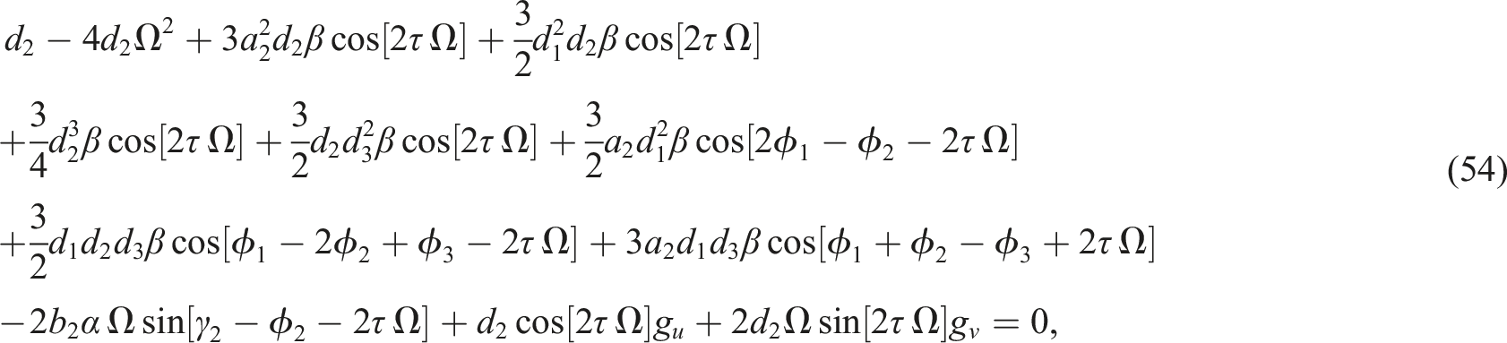
Substituting equation (42) and equation (44) into equation (43), we can get the following equations

L_{4} (x_{1, 1}) = [\begin{array}{l} - b_{1} Ω^{2} \cos (Ω t + ϕ_{1}) - 4 b_{2} Ω^{2} \cos (2 Ω t + ϕ_{2}) - 9 b_{3} Ω^{2} \cos (3 Ω t + ϕ_{3}) \\ - 2 ζ b_{1} Ω \sin (Ω t + ϕ_{1}) - 4 ζ b_{2} Ω \sin (2 Ω t + ϕ_{2}) - 6 ζ b_{3} Ω \sin (3 Ω t + ϕ_{3}) \\ + a_{1} + b_{1} \cos (Ω t + ϕ_{1}) + b_{2} \cos 2 Ω t + ϕ_{2}) + b_{3} \cos (3 Ω t + ϕ_{3}) + g_{u} a_{1} \\ + g_{u} b_{1} \cos (Ω t - Ω τ + ϕ_{1}) + g_{u} b_{2} \cos (2 Ω t - 2 Ω τ + ϕ_{2}) \\ + g_{u} b_{3} \cos (3 Ω t - 3 Ω τ + ϕ_{3}) + g_{v} (- b_{1} Ω \sin (Ω t - Ω τ + ϕ_{1}) \\ - 2 b_{2} Ω \sin (2 Ω t - 2 Ω τ + ϕ_{2}) - 3 b_{3} Ω \sin (3 Ω t - 3 Ω τ + ϕ_{3})) \\ - α (- d_{1} Ω \sin (Ω t - Ω τ + γ_{1}) - 2 d_{2} Ω \sin (2 Ω t - 2 Ω τ + γ_{2}) \\ - 3 d_{3} Ω \sin (3 Ω t - 3 Ω τ + γ_{3})) - β (a_{1} + b_{1} \cos (Ω t - Ω τ + ϕ_{1}) \\ {+ b_{2} \cos (2 Ω t - 2 Ω τ + ϕ_{2}) + b_{3} \cos (3 Ω t - 3 Ω τ + ϕ_{3}))}^{3} \end{array}] ℏ,

(45)

L_{4} (y_{1, 1}) = [\begin{array}{l} - d_{1} Ω^{2} \cos (Ω t + γ_{1}) - 4 d_{2} Ω^{2} \cos (2 Ω t + γ_{2}) - 9 d_{3} Ω^{2} \cos (3 Ω t + γ_{3}) \\ - 2 ζ d_{1} Ω \sin (Ω t + γ_{1}) - 4 ζ d_{2} Ω \sin (2 Ω t + γ_{2}) - 6 ζ d_{3} Ω \sin (3 Ω t + γ_{3}) \\ + a_{2} + d_{1} \cos (Ω t + γ_{1}) + d_{2} \cos (2 Ω t + γ_{2}) + d_{3} \cos (3 Ω t + γ_{3}) + g_{u} a_{2} \\ + g_{u} d_{1} \cos (Ω t - Ω τ + γ_{1}) + g_{u} d_{2} \cos (2 Ω t - 2 Ω τ + γ_{2}) \\ + g_{u} d_{3} \cos (3 Ω t - 3 Ω τ + γ_{3}) + g_{v} (- d_{1} Ω \sin (Ω t - Ω τ + γ_{1}) \\ - 2 d_{2} Ω \sin (2 Ω t - 2 Ω τ + γ_{2}) - 3 d_{3} Ω \sin (3 Ω t - 3 Ω τ + γ_{3})) \\ - α (- b_{1} Ω \sin (Ω t - Ω τ + γ_{1}) - 2 b_{2} Ω \sin (2 Ω t - 2 Ω τ + γ_{2}) \\ - 3 b_{3} Ω \sin (3 Ω t - 3 Ω τ + γ_{3})) - β (a_{2} + d_{1} \cos (Ω t - Ω τ + γ_{1}) \\ {+ d_{2} \cos (2 Ω t - 2 Ω τ + γ_{2}) + d_{3} \cos (3 Ω t - 3 Ω τ + γ_{3}))}^{3} \end{array}] ℏ .

(46)

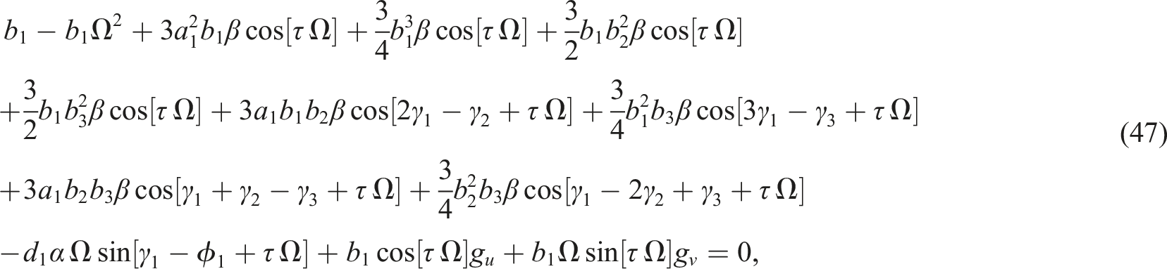
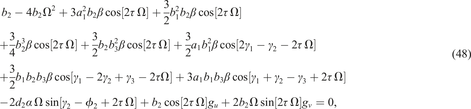
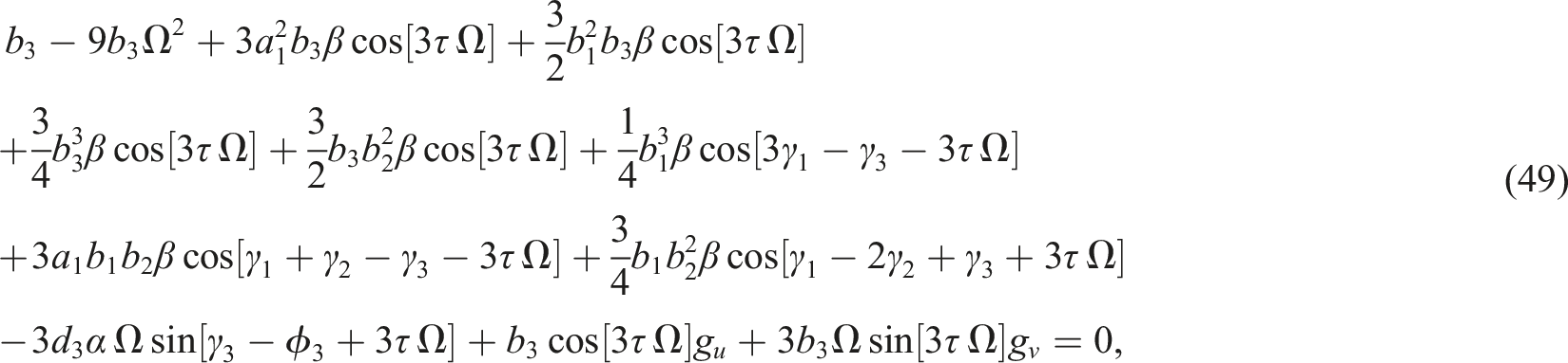
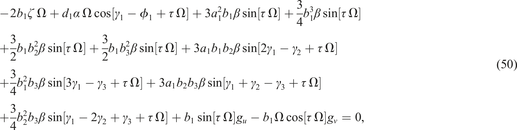
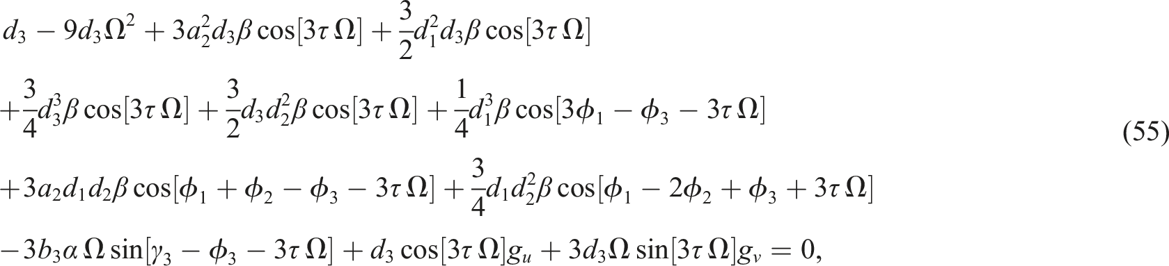
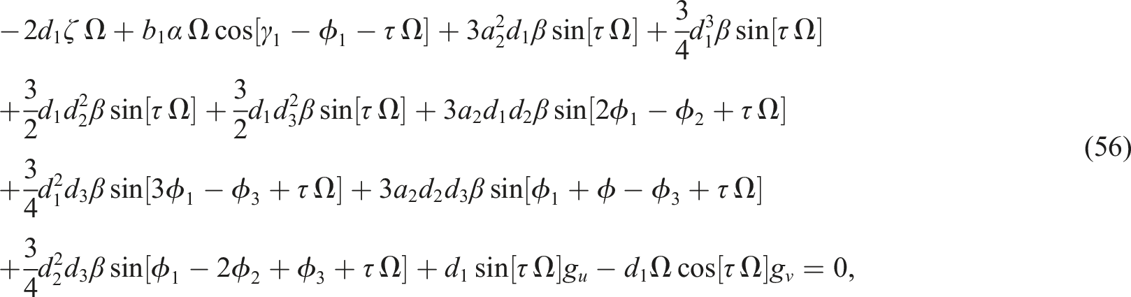
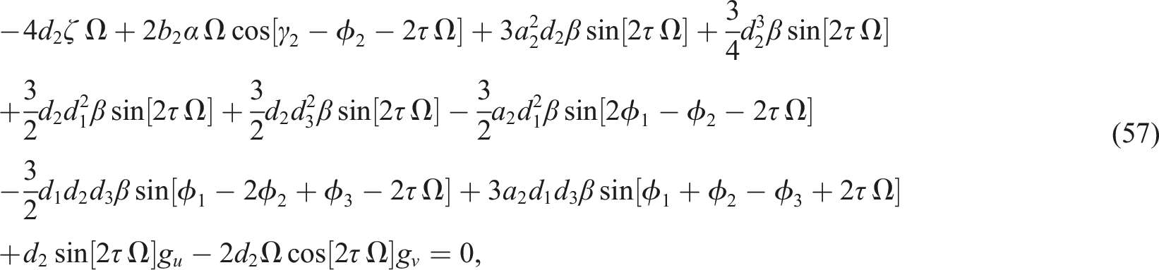
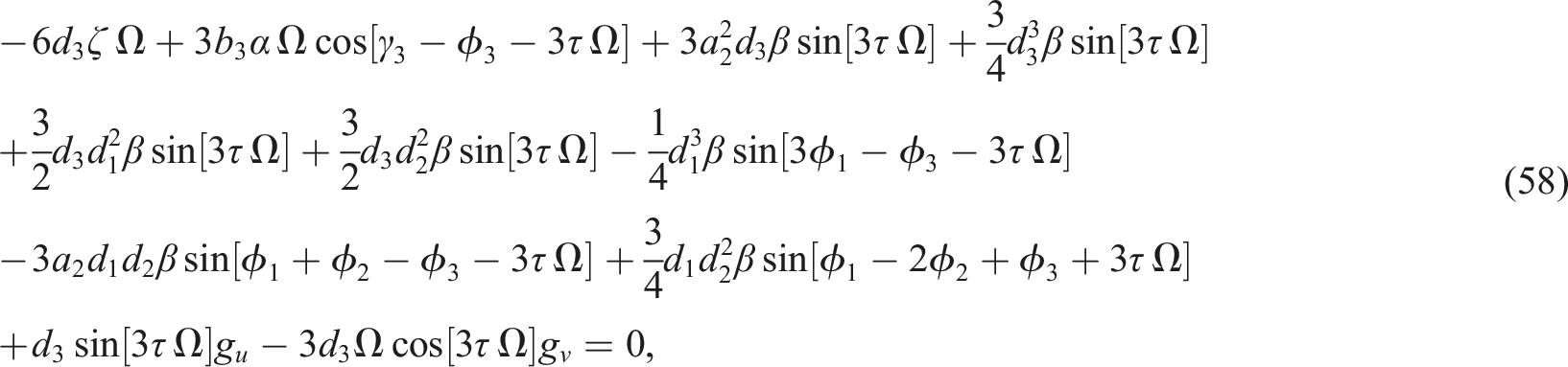
To eliminate the secular terms in x_1,1, y_1,1, expand equation (45) and equation (46), we can obtain the equations as follows.

\begin{array}{l} b_{1} - b_{1} Ω^{2} + 3 a_{1}^{2} b_{1} β \cos [τ Ω] + \frac{3}{4} b_{1}^{3} β \cos [τ Ω] + \frac{3}{2} b_{1} b_{2}^{2} β \cos [τ Ω] \\ + \frac{3}{2} b_{1} b_{3}^{2} β \cos [τ Ω] + 3 a_{1} b_{1} b_{2} β \cos [2 γ_{1} - γ_{2} + τ Ω] + \frac{3}{4} b_{1}^{2} b_{3} β \cos [3 γ_{1} - γ_{3} + τ Ω] \\ + 3 a_{1} b_{2} b_{3} β \cos [γ_{1} + γ_{2} - γ_{3} + τ Ω] + \frac{3}{4} b_{2}^{2} b_{3} β \cos [γ_{1} - 2 γ_{2} + γ_{3} + τ Ω] \\ - d_{1} α Ω \sin [γ_{1} - ϕ_{1} + τ Ω] + b_{1} \cos [τ Ω] g_{u} + b_{1} Ω \sin [τ Ω] g_{v} = 0, \end{array}

(47)

\begin{array}{l} b_{2} - 4 b_{2} Ω^{2} + 3 a_{1}^{2} b_{2} β \cos [2 τ Ω] + \frac{3}{2} b_{1}^{2} b_{2} β \cos [2 τ Ω] \\ + \frac{3}{4} b_{2}^{3} β \cos [2 τ Ω] + \frac{3}{2} b_{2} b_{3}^{2} β \cos [2 τ Ω] + \frac{3}{2} a_{1} b_{1}^{2} β \cos [2 γ_{1} - γ_{2} - 2 τ Ω] \\ + \frac{3}{2} b_{1} b_{2} b_{3} β \cos [γ_{1} - 2 γ_{2} + γ_{3} - 2 τ Ω] + 3 a_{1} b_{1} b_{3} β \cos [γ_{1} + γ_{2} - γ_{3} + 2 τ Ω] \\ - 2 d_{2} α Ω \sin [γ_{2} - ϕ_{2} + 2 τ Ω] + b_{2} \cos [2 τ Ω] g_{u} + 2 b_{2} Ω \sin [2 τ Ω] g_{v} = 0, \end{array}

(48)

\begin{array}{l} b_{3} - 9 b_{3} Ω^{2} + 3 a_{1}^{2} b_{3} β \cos [3 τ Ω] + \frac{3}{2} b_{1}^{2} b_{3} β \cos [3 τ Ω] \\ + \frac{3}{4} b_{3}^{3} β \cos [3 τ Ω] + \frac{3}{2} b_{3} b_{2}^{2} β \cos [3 τ Ω] + \frac{1}{4} b_{1}^{3} β \cos [3 γ_{1} - γ_{3} - 3 τ Ω] \\ + 3 a_{1} b_{1} b_{2} β \cos [γ_{1} + γ_{2} - γ_{3} - 3 τ Ω] + \frac{3}{4} b_{1} b_{2}^{2} β \cos [γ_{1} - 2 γ_{2} + γ_{3} + 3 τ Ω] \\ - 3 d_{3} α Ω \sin [γ_{3} - ϕ_{3} + 3 τ Ω] + b_{3} \cos [3 τ Ω] g_{u} + 3 b_{3} Ω \sin [3 τ Ω] g_{v} = 0, \end{array}

(49)

\begin{array}{l} - 2 b_{1} ζ Ω + d_{1} α Ω \cos [γ_{1} - ϕ_{1} + τ Ω] + 3 a_{1}^{2} b_{1} β \sin [τ Ω] + \frac{3}{4} b_{1}^{3} β \sin [τ Ω] \\ + \frac{3}{2} b_{1} b_{2}^{2} β \sin [τ Ω] + \frac{3}{2} b_{1} b_{3}^{2} β \sin [τ Ω] + 3 a_{1} b_{1} b_{2} β \sin [2 γ_{1} - γ_{2} + τ Ω] \\ + \frac{3}{4} b_{1}^{2} b_{3} β \sin [3 γ_{1} - γ_{3} + τ Ω] + 3 a_{1} b_{2} b_{3} β \sin [γ_{1} + γ_{2} - γ_{3} + τ Ω] \\ + \frac{3}{4} b_{2}^{2} b_{3} β \sin [γ_{1} - 2 γ_{2} + γ_{3} + τ Ω] + b_{1} \sin [τ Ω] g_{u} - b_{1} Ω \cos [τ Ω] g_{v} = 0, \end{array}

(50)

\begin{array}{l} - 4 b_{2} ζ Ω + 2 d_{2} α Ω \cos [γ_{2} - ϕ_{2} + 2 τ Ω] + 3 a_{1}^{2} b_{2} β \sin [2 τ Ω] + \frac{3}{4} b_{2}^{3} β \sin [2 τ Ω] \\ + \frac{3}{2} b_{2} b_{1}^{2} β \sin [2 τ Ω] + \frac{3}{2} b_{2} b_{3}^{2} β \sin [2 τ Ω] - \frac{3}{2} a_{1} b_{1}^{2} β \sin [2 γ_{1} - γ_{2} - 2 τ Ω] \\ - \frac{3}{2} b_{1} b_{2} b_{3} β \sin [γ_{1} - 2 γ_{2} + γ_{3} - 2 τ Ω] + 3 a_{1} b_{1} b_{3} β \sin [γ_{1} + γ_{2} - γ_{3} + 2 τ Ω] \\ + b_{2} \sin [2 τ Ω] g_{u} - 2 b_{2} Ω \cos [2 τ Ω] g_{v} = 0, \end{array}

(51)

\begin{array}{l} - 6 b_{3} ζ Ω + 3 d_{3} α Ω \cos [γ_{3} - ϕ_{3} + 3 τ Ω] + 3 a_{1}^{2} b_{3} β \sin [3 τ Ω] + \frac{3}{4} b_{3}^{3} β \sin [3 τ Ω] \\ + \frac{3}{2} b_{3} b_{1}^{2} β \sin [3 τ Ω] + \frac{3}{2} b_{3} b_{2}^{2} β \sin [3 τ Ω] - \frac{1}{4} b_{1}^{3} β \sin [3 γ_{1} - γ_{3} - 3 τ Ω] \\ - 3 a_{1} b_{1} b_{2} β \sin [γ_{1} + γ_{2} - γ_{3} - 3 τ Ω] + \frac{3}{4} b_{1} b_{2}^{2} β \sin [γ_{1} - 2 γ_{2} + γ_{3} + 3 τ Ω] \\ + b_{3} \sin [3 τ Ω] g_{u} - 3 b_{3} Ω \cos [3 τ Ω] g_{v} = 0, \end{array}

(52)

\begin{array}{l} d_{1} - d_{1} Ω^{2} + 3 a_{2}^{2} d_{1} β \cos [τ Ω] + \frac{3}{4} d_{1}^{3} β \cos [τ Ω] + \frac{3}{2} d_{1} d_{2}^{2} β \cos [τ Ω] \\ + \frac{3}{2} d_{1} d_{3}^{2} β \cos [τ Ω] + 3 a_{2} d_{1} d_{2} β \cos [2 ϕ_{1} - ϕ_{2} + τ Ω] + \frac{3}{4} d_{1}^{2} d_{3} β \cos [3 ϕ_{1} - ϕ_{3} + τ Ω] \\ + 3 a_{2} d_{2} d_{3} β \cos [ϕ_{1} + ϕ_{2} - ϕ_{3} + τ Ω] + \frac{3}{4} d_{2}^{2} d_{3} β \cos [ϕ_{1} - 2 ϕ_{2} + ϕ_{3} + τ Ω] \\ - b_{1} α Ω \sin [γ_{1} - ϕ_{1} - τ Ω] + d_{1} \cos [τ Ω] g_{u} + d_{1} Ω \sin [τ Ω] g_{v} = 0, \end{array}

(53)

\begin{array}{l} d_{2} - 4 d_{2} Ω^{2} + 3 a_{2}^{2} d_{2} β \cos [2 τ Ω] + \frac{3}{2} d_{1}^{2} d_{2} β \cos [2 τ Ω] \\ + \frac{3}{4} d_{2}^{3} β \cos [2 τ Ω] + \frac{3}{2} d_{2} d_{3}^{2} β \cos [2 τ Ω] + \frac{3}{2} a_{2} d_{1}^{2} β \cos [2 ϕ_{1} - ϕ_{2} - 2 τ Ω] \\ + \frac{3}{2} d_{1} d_{2} d_{3} β \cos [ϕ_{1} - 2 ϕ_{2} + ϕ_{3} - 2 τ Ω] + 3 a_{2} d_{1} d_{3} β \cos [ϕ_{1} + ϕ_{2} - ϕ_{3} + 2 τ Ω] \\ - 2 b_{2} α Ω \sin [γ_{2} - ϕ_{2} - 2 τ Ω] + d_{2} \cos [2 τ Ω] g_{u} + 2 d_{2} Ω \sin [2 τ Ω] g_{v} = 0, \end{array}

(54)

\begin{array}{l} d_{3} - 9 d_{3} Ω^{2} + 3 a_{2}^{2} d_{3} β \cos [3 τ Ω] + \frac{3}{2} d_{1}^{2} d_{3} β \cos [3 τ Ω] \\ + \frac{3}{4} d_{3}^{3} β \cos [3 τ Ω] + \frac{3}{2} d_{3} d_{2}^{2} β \cos [3 τ Ω] + \frac{1}{4} d_{1}^{3} β \cos [3 ϕ_{1} - ϕ_{3} - 3 τ Ω] \\ + 3 a_{2} d_{1} d_{2} β \cos [ϕ_{1} + ϕ_{2} - ϕ_{3} - 3 τ Ω] + \frac{3}{4} d_{1} d_{2}^{2} β \cos [ϕ_{1} - 2 ϕ_{2} + ϕ_{3} + 3 τ Ω] \\ - 3 b_{3} α Ω \sin [γ_{3} - ϕ_{3} - 3 τ Ω] + d_{3} \cos [3 τ Ω] g_{u} + 3 d_{3} Ω \sin [3 τ Ω] g_{v} = 0, \end{array}

(55)

\begin{array}{l} - 2 d_{1} ζ Ω + b_{1} α Ω \cos [γ_{1} - ϕ_{1} - τ Ω] + 3 a_{2}^{2} d_{1} β \sin [τ Ω] + \frac{3}{4} d_{1}^{3} β \sin [τ Ω] \\ + \frac{3}{2} d_{1} d_{2}^{2} β \sin [τ Ω] + \frac{3}{2} d_{1} d_{3}^{2} β \sin [τ Ω] + 3 a_{2} d_{1} d_{2} β \sin [2 ϕ_{1} - ϕ_{2} + τ Ω] \\ + \frac{3}{4} d_{1}^{2} d_{3} β \sin [3 ϕ_{1} - ϕ_{3} + τ Ω] + 3 a_{2} d_{2} d_{3} β \sin [ϕ_{1} + ϕ - ϕ_{3} + τ Ω] \\ + \frac{3}{4} d_{2}^{2} d_{3} β \sin [ϕ_{1} - 2 ϕ_{2} + ϕ_{3} + τ Ω] + d_{1} \sin [τ Ω] g_{u} - d_{1} Ω \cos [τ Ω] g_{v} = 0, \end{array}

(56)

\begin{array}{l} - 4 d_{2} ζ Ω + 2 b_{2} α Ω \cos [γ_{2} - ϕ_{2} - 2 τ Ω] + 3 a_{2}^{2} d_{2} β \sin [2 τ Ω] + \frac{3}{4} d_{2}^{3} β \sin [2 τ Ω] \\ + \frac{3}{2} d_{2} d_{1}^{2} β \sin [2 τ Ω] + \frac{3}{2} d_{2} d_{3}^{2} β \sin [2 τ Ω] - \frac{3}{2} a_{2} d_{1}^{2} β \sin [2 ϕ_{1} - ϕ_{2} - 2 τ Ω] \\ - \frac{3}{2} d_{1} d_{2} d_{3} β \sin [ϕ_{1} - 2 ϕ_{2} + ϕ_{3} - 2 τ Ω] + 3 a_{2} d_{1} d_{3} β \sin [ϕ_{1} + ϕ_{2} - ϕ_{3} + 2 τ Ω] \\ + d_{2} \sin [2 τ Ω] g_{u} - 2 d_{2} Ω \cos [2 τ Ω] g_{v} = 0, \end{array}

(57)

\begin{array}{l} - 6 d_{3} ζ Ω + 3 b_{3} α Ω \cos [γ_{3} - ϕ_{3} - 3 τ Ω] + 3 a_{2}^{2} d_{3} β \sin [3 τ Ω] + \frac{3}{4} d_{3}^{3} β \sin [3 τ Ω] \\ + \frac{3}{2} d_{3} d_{1}^{2} β \sin [3 τ Ω] + \frac{3}{2} d_{3} d_{2}^{2} β \sin [3 τ Ω] - \frac{1}{4} d_{1}^{3} β \sin [3 ϕ_{1} - ϕ_{3} - 3 τ Ω] \\ - 3 a_{2} d_{1} d_{2} β \sin [ϕ_{1} + ϕ_{2} - ϕ_{3} - 3 τ Ω] + \frac{3}{4} d_{1} d_{2}^{2} β \sin [ϕ_{1} - 2 ϕ_{2} + ϕ_{3} + 3 τ Ω] \\ + d_{3} \sin [3 τ Ω] g_{u} - 3 d_{3} Ω \cos [3 τ Ω] g_{v} = 0, \end{array}

(58)

\begin{array}{l} a_{1} + a_{1} g_{u} + a_{1}^{3} β + \frac{3}{2} a_{1} b_{1}^{2} β + \frac{3}{2} a_{1} b_{2}^{2} β + \frac{3}{2} a_{1} b_{3}^{2} β + \frac{3}{4} b_{1}^{2} b_{2} β \cos [2 γ_{1} - γ_{2}] \\ + \frac{3}{2} b_{1} b_{2} b_{3} β \cos [γ_{1} + γ_{2} - γ_{3}] = 0, \end{array}

(59)

\begin{array}{l} a_{2} + a_{2} g_{u} + a_{2}^{3} β + \frac{3}{2} a_{2} d_{1}^{2} β + \frac{3}{2} a_{2} d_{2}^{2} β + \frac{3}{2} a_{2} d_{3}^{2} β + \frac{3}{4} d_{1}^{2} d_{2} β \cos [2 ϕ_{1} - ϕ_{2}] \\ + \frac{3}{2} d_{1} d_{2} d_{3} β \cos [ϕ_{1} + ϕ_{2} - ϕ_{3}] = 0 . \end{array}

(60)

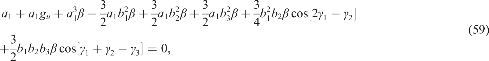
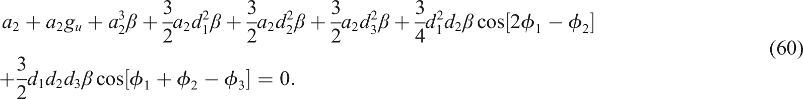
After eliminating the secular terms, we can get the expression of x_1,1 and y_1,1, where the parameters a₁, a₂, b_i, d_i, ϕ_i, and γ_i (i = 1, 2, 3) can be calculated by equations. (47) to (60) and then the solution x_1,1 and y_1,1 can be obtained.

Thus, the first-order approximate solutions of x₁ and y₁ are, respectively

\begin{array}{l} x_{1} (t) = \lim_{q \to 1} (x_{0} + q x_{1}) = x_{1, 0} + x_{1, 1}, \\ y_{1} (t) = \lim_{q \to 1} (y_{0} + q y_{1}) = y_{1, 0} + y_{1, 1} . \end{array}

(61)

For the period-doubling solution, the characteristic polynomial is

P (λ) = λ \prod_{r = 1}^{6} (λ + \frac{r Ω}{2} i) (λ - \frac{r Ω}{2} i)

(62)

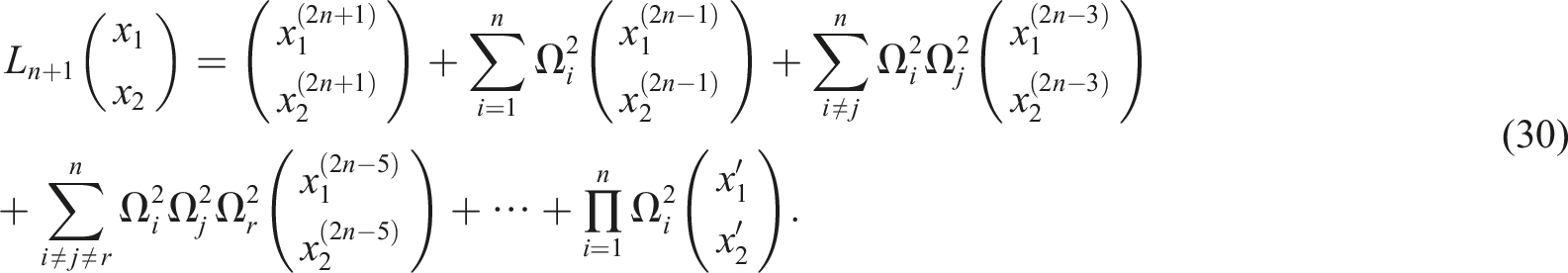
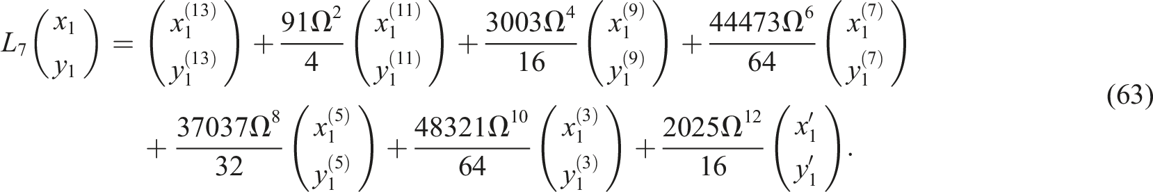
The corresponding auxiliary linear differential operator is as follows:

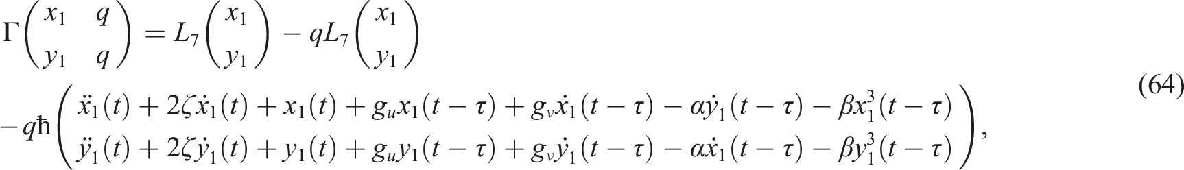
\begin{array}{l} L_{7} (\begin{array}{l} x_{1} \\ y_{1} \end{array}) = (\begin{array}{l} x_{1}^{(13)} \\ y_{1}^{(13)} \end{array}) + \frac{91 Ω^{2}}{4} (\begin{array}{l} x_{1}^{(11)} \\ y_{1}^{(11)} \end{array}) + \frac{3003 Ω^{4}}{16} (\begin{array}{l} x_{1}^{(9)} \\ y_{1}^{(9)} \end{array}) + \frac{44473 Ω^{6}}{64} (\begin{array}{l} x_{1}^{(7)} \\ y_{1}^{(7)} \end{array}) \\ + \frac{37037 Ω^{8}}{32} (\begin{array}{l} x_{1}^{(5)} \\ y_{1}^{(5)} \end{array}) + \frac{48321 Ω^{10}}{64} (\begin{array}{l} x_{1}^{(3)} \\ y_{1}^{(3)} \end{array}) + \frac{2025 Ω^{12}}{16} (\begin{array}{l} x_{1}^{'} \\ y_{1}^{'} \end{array}) . \end{array}

(63)

next, we construct the homotopy expression

\begin{array}{l} Γ (\begin{array}{l} x_{1} & q \\ y_{1} & q \end{array}) = L_{7} (\begin{array}{l} x_{1} \\ y_{1} \end{array}) - q L_{7} (\begin{array}{l} x_{1} \\ y_{1} \end{array}) \\ - q ℏ (\begin{array}{l} {\ddot{x}}_{1} (t) + 2 ζ {\dot{x}}_{1} (t) + x_{1} (t) + g_{u} x_{1} (t - τ) + g_{v} {\dot{x}}_{1} (t - τ) - α {\dot{y}}_{1} (t - τ) - β x_{1}^{3} (t - τ) \\ {\ddot{y}}_{1} (t) + 2 ζ {\dot{y}}_{1} (t) + y_{1} (t) + g_{u} y_{1} (t - τ) + g_{v} {\dot{y}}_{1} (t - τ) - α {\dot{x}}_{1} (t - τ) - β y_{1}^{3} (t - τ) \end{array}), \end{array}

(64)

where ℏ is the auxiliary parameter and q∈[0,1] is the embedding variable.

Assuming that the solution of equation (1) can be expressed as

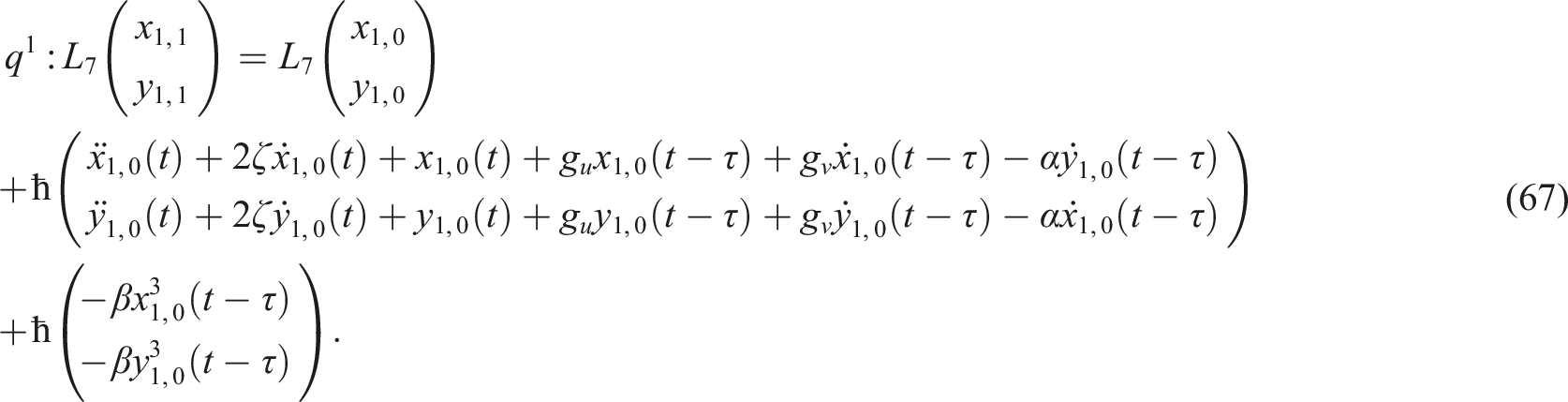
\begin{array}{l} x_{1} = x_{1, 0} + q x_{1, 1} + q^{2} x_{1, 2} + \dots, \\ y_{1} = x_{1, 0} + q y_{1, 1} + q^{2} y_{1, 2} + \dots . \end{array}

(65)

Substituting equation (65) into equation (64) and eliminating the same power terms of q, we can get

q^{0} : L_{7} (\begin{array}{l} x_{1, 0} \\ y_{1, 0} \end{array}) = 0

(66)

\begin{array}{l} q^{1} : L_{7} (\begin{array}{l} x_{1, 1} \\ y_{1, 1} \end{array}) = L_{7} (\begin{array}{l} x_{1, 0} \\ y_{1, 0} \end{array}) \\ + ℏ (\begin{array}{l} {\ddot{x}}_{1, 0} (t) + 2 ζ {\dot{x}}_{1, 0} (t) + x_{1, 0} (t) + g_{u} x_{1, 0} (t - τ) + g_{v} {\dot{x}}_{1, 0} (t - τ) - α {\dot{y}}_{1, 0} (t - τ) \\ {\ddot{y}}_{1, 0} (t) + 2 ζ {\dot{y}}_{1, 0} (t) + y_{1, 0} (t) + g_{u} y_{1, 0} (t - τ) + g_{v} {\dot{y}}_{1, 0} (t - τ) - α {\dot{x}}_{1, 0} (t - τ) \end{array}) \\ + ℏ (\begin{array}{l} - β x_{1, 0}^{3} (t - τ) \\ - β y_{1, 0}^{3} (t - τ) \end{array}) . \end{array}

(67)

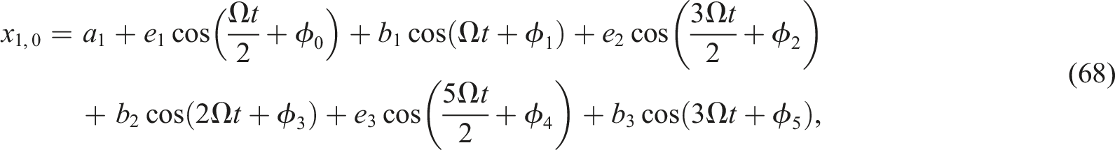
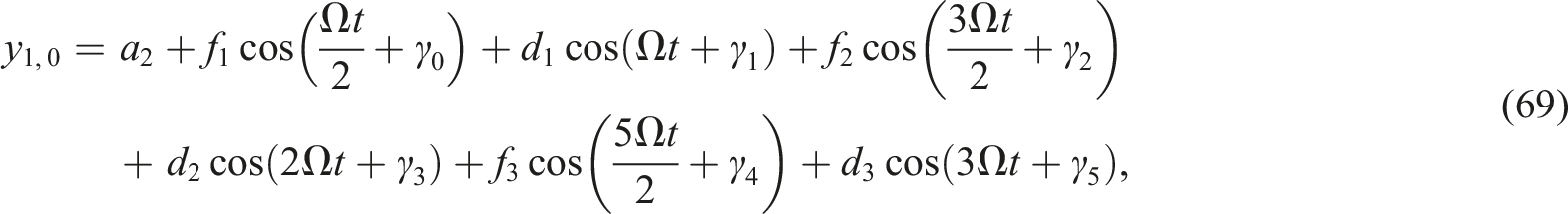
Assuming that the solution of equation (66) can be expressed by

\begin{array}{l} x_{1, 0} = a_{1} + e_{1} \cos (\frac{Ω t}{2} + ϕ_{0}) + b_{1} \cos (Ω t + ϕ_{1}) + e_{2} \cos (\frac{3 Ω t}{2} + ϕ_{2}) \\ + b_{2} \cos (2 Ω t + ϕ_{3}) + e_{3} \cos (\frac{5 Ω t}{2} + ϕ_{4}) + b_{3} \cos (3 Ω t + ϕ_{5}), \end{array}

(68)

\begin{array}{l} y_{1, 0} = a_{2} + f_{1} \cos (\frac{Ω t}{2} + γ_{0}) + d_{1} \cos (Ω t + γ_{1}) + f_{2} \cos (\frac{3 Ω t}{2} + γ_{2}) \\ + d_{2} \cos (2 Ω t + γ_{3}) + f_{3} \cos (\frac{5 Ω t}{2} + γ_{4}) + d_{3} \cos (3 Ω t + γ_{5}), \end{array}

(69)

where a₁, a₂, b_i, d_i, e_i, f_i, ϕ_j, γ_j(i = 1, 2, 3)(j = 1, 2, 3, 4, 5) are unknown parameters.

Substituting equations (68) and (69) and (66) into (67), and eliminating the secular term in x_1,1(t), y_1,1(t), we can get some equations of a₁, a₂, b_i, d_i, e_i, f_i, ϕ_j, γ_j(i = 1, 2, 3)(j = 1, 2, 3, 4, 5). After solving these equations, we can get the value of a₁, a₂, b_i, d_i, e_i, f_i, ϕ_j, γ_j(i = 1, 2, 3)(j = 1, 2, 3, 4, 5). Then the double period solution can be obtained.

Numerical simulation

In this section, we get the approximate solution by using the MFHAM and compare it with the fourth-order Runge–Kutta method. According to the normal form section, when parameters are chosen in region II, system (1) has an unstable periodic solution. In regions III and V, system (1) has two unstable periodic motions. When (α_ε,τ_ε) is located in region IV, system (1) has a stable periodic solution and an unstable periodic motion. For region VI, system (1) admits an unstable solution.

Set g_u = 0, $g_{v} = \sqrt{15} / 5$ , ζ = 0, and β = 0.1, then when parameters fall in region II, α = −0.727489, τ = 5.083668, h = −1, and Ω = 0.6, we get unstable periodic solution of the system, which can be seen through the phase portrait and time history diagram in Figure 6.when parameters fall in region III, α = −1.092, τ = 5.083668, h = −1, and Ω = 0.9, we get the phase portrait and time history diagram of unstable periodic solution in Figure 7.when parameters fall in region IV, α = −0.258, τ = 100.08, h = −1, and Ω = 1.0, a stable periodic motion of system is obtained as shown in Figure 8. And through comparison of the approximate analytical solution and numerical solution, we can see the approximate solution is in a good agreement with the numerical solution.when parameters fall in region V, α = −0.9993, τ = 5.083668, h = −1, and Ω = 1.1, the approximate analytical solution of periodic motion is also obtained as shown in Figure 9.when parameters fall in region VI, α = −0.038, τ = 7.083668, h = −1, and Ω = 0.6, we get unstable limit cycle generated by the system in Figure 10.

Figure 6.

Unstable period solution of the time delay coupled active control system, (a) the phase portrait MFHAM approximate solution and (b) the time history MFHAM approximate solution.

Figure 7.

Unstable period solution of the time delay coupled active control system: (a) the phase portrait MFHAM approximate solution and (b) the time history MFHAM approximate solution.

Figure 8.

Stable period solution of the time delay coupled active control system: (a) the phase portrait MFHAM approximate solution ——RK solution and (b) the time history MFHAM approximate solution ——RK solution.

Figure 9.

Unstable period solution of the time delay coupled active control system: (a) the phase portrait MFHAM approximate solution and (b) the time history MFHAM approximate solution.

Figure 10.

Unstable period solution of the time delay coupled active control system: (a) the phase portrait MFHAM approximate solution and (b) the time history MFHAM approximate solution.

Conclusion

This paper investigates the effect of time delay and coupling strength on the time delay coupled active control system. Here, we focus on the stability of the equilibrium point and the existence of the double Hopf bifurcation. Firstly, we used the characteristic equation to analyze the stability of the system and obtained the stability switching region of the system with respect to the delay. The results show that the time delay affected the stability of the equilibrium point. Secondly, in order to study the dynamics near the bifurcation point, we obtained the normal form of double Hopf bifurcation, from which the bifurcation analysis of the critical point is given. Based on the bifurcation analysis, the parameter region of the stable periodic solution and the stable quasi-periodic solution are obtained. It is concluded that the time delay is not negligible in the coupled active control system, and the change of the coupling strength also affects the dynamical behavior of the system. Finally, the periodic solutions of the system were solved by MFHAM to verify the existence of unstable periodic solutions. The results of this paper are useful for the study of the dynamics of time delay coupled systems.

Footnotes

Acknowledgments

The authors gratefully acknowledge the reviewers for their comments.

Author contributions

Conceptualization, Y.Q.; methodology, Y.Q.; writing—review and editing, Y.Q.; supervision, Y.Q.; funding acquisition, Y.Q.; conceptualization, H.Z.; methodology, H.Z.; writing—original draft preparation, H.Z.; writing—review and editing, H.Z.; software, H.Z.

Declaration of conflicting interests

The author(s) declared no potential conflicts of interest with respect to the research, authorship, and/or publication of this article.

Funding

The author(s) disclosed receipt of the following financial support for the research, authorship, and/or publication of this article: National Natural Science Foundation of China (NNSFC) through grant no. 12172333 and Natural Science Foundation of ZheJiang through grant no. LY20A020003.

ORCID iD

Youhua Qian

References

Zhou

Chen

. Two fast/slow decompositions as well as period-adding sequences in a generalized Bonhoeffer-van der Pol electronic circuit. AEU-Int J Electron C 2022; 155: 154379.

Wang

Zhang

, et al. Melnikov-threshold-triggered mixed-mode oscillations in a family of amplitude-modulated forced oscillator. J Low Freq Noise V A 2019; 38(2): 377–387.

Zhang

Chen

, et al. Relaxation and mixed mode oscillations in a shape memory alloy oscillator driven by parametric and external excitations. Chaos Soliton Fract 2020; 140: 110145.

. Analysis on double Hopf bifurcation using computer Algebra with the Aid of multiple scales. Nonlinear Dyn 2002; 27(1): 19–53.

Feng

. Double Hopf bifurcation for van der Pol-Duffing oscillator with parametric delay feedback control. J Math Anal Appl 2008; 338(2): 993–1007.

Itovich

Moiola

. Double Hopf bifurcation analysis using frequency domain methods. Nonlinear Dyn 2015; 39(3): 235–258.

Peng

Wang

Zhao

, et al. Bifurcation analysis in active control system with time delay feedback. Appl Math Comput 2013; 219(19): 10073–10081.

Ding

Cao

Jiang

. Double Hopf bifurcation in active control system with delayed feedback: application to glue dosing processes for particleboard. Nonlinear Dyn 2016; 83(3): 1567–1576.

Sun

Jing

, et al. Beneficial performance of a quasi-zero-stiffness vibration isolator with time-delayed active control. Int J Mech Sci 2014; 82: 32–40.

10.

Xing

Xiao

Zhang

, et al. Stability and Hopf bifurcation analysis of an (n+ m)-neuron double-ring neural network model with multiple time delays. J Syst Sci Complex 2022; 35(1): 159–178.

11.

. Stability and Hopf bifurcation on four-neuron neural networks with inertia and multiple delays. Neurocomputing 2018; 287: 34–44.

12.

Yan

Chu

. Stability and bifurcation analysis for a delayed LotkaCVolterra predatorCprey system. J Comput Appl Math 2006; 196(1): 198–210.

13.

Liu

Wei

. Double Hopf bifurcation of a diffusive predatorCprey system with strong Allee effect and two delays. Nonlinear Anal-Model 2021; 26(1): 72–92.

14.

. An analytical method for studying double Hopf bifurcations induced by two delays in nonlinear differential systems. Sci China Tech Sci 2020; 63(4): 597–602.

15.

Song

Peng

Zhang

. Double Hopf bifurcation analysis in the memory-based diffusion system. J Dyn Differ Equ 2022: 1–42.

16.

Qian

Guo

. Weakly resonant double Hopf bifurcation in coupled nonlinear systems with delayed freedback and application of homotopy analysis method. J Low Freq Noise V A 2019; 38(3-4): 1651–1675.

17.

. Weak resonant double Hopf bifurcations in an inertial four-neuron model with time delay. Int J Neural Syst 2012; 22(01): 63–75.

18.

Zhou

Qian

. Double Hopf bifurcation analysis for coupled van der Pol-Rayleigh system with time delay. J Vib Eng Technol 2023, Online ahead of print. DOI: 10.1007/s42417-023-01238-3.

19.

Liao

. The proposed homotopy analysis technique for the solution of nonlinear problems. Shanghai Jiao Tong University Shanghai, 1992.

20.

You

. Analytical approximations for the periodic motion of the Duffing system with delayed feedback. Numer Algorithms 2011; 56(4): 561–576.

21.

Jafarian

Ghaderi

Golmankhaneh

, et al. Homotopy analysis method for solving coupled Ramani equations. Rom J Phys 2014; 59(1-2): 26–35.

22.

Zhou

Chang

. Nonlinear vibration analysis of functionally graded flow pipelines under generalized boundary conditions based on homotopy analysis. Acta Mech 2022; 233(12): 5447C5463.

23.

Song

Shao

Zhang

. Residue-regulating homotopy method for strongly nonlinear oscillators. Nonlinear Dyn 2022; 109(3): 1905–1921.

24.

Yan

Wang

. Time-delay feedback control of a cantilever beam with concentrated mass based on the homotopy analysis method. Appl Math Model 2022; 108: 629–645.

25.

Xie

, et al. Explicit solution to large deformation of cantilever beam by improved homotopy analysis method II: vertical and horizontal displacements. Appl Sci 2022; 12(5): 2513.

26.

Zhu

. Power series approximation solution to thermoelectric generator temperature field by homotopy analysis method. J Electron Mater 2023; 52(3): 1–9.

27.

Zou

Nagarajaiah

. The solution structure of the Dffing oscillators transient response and general solution. Nonlinear Dyn 2015; 81: 621–639.

28.

Qian

. Study on a multi-frequency homotopy analysis method for period-doubling solutions of nonlinear systems. Int J Bifurcat Chaos 2018; 28(04): 1850049.

29.

Qiang

Qian

Guo

. Periodic solutions of delay nonlinear system by multi-frequency homotopy analysis method. J Low Freq Noise V A 2019; 38(3-4): 1439–1454.

30.

Peng

Zhang

, et al. Qualitative analysis in a delayed Van der Pol oscillator. Phys A 2020; 544: 123482.

Double Hopf bifurcation analysis of time delay coupled active control system

Abstract

Keywords

Introduction

Stability analysis

Model

Stability switches: Case one

Stability switches: Case two

The normal form

Multi-frequency Homotopy Analysis Method

Analyzing the time delay coupled active control system with MFHAM

Numerical simulation

Conclusion

Footnotes

Acknowledgments

Author contributions

Declaration of conflicting interests

Funding

ORCID iD

References