Sage Journals: Discover world-class research

Abstract

An on-site system for measuring low-frequency noise and complainant's responses to the low-frequency noise was developed to confirm whether the complainant suffer from the environmental noise with low-frequency components. The system suggests several methods to find the dominant frequency and major sound pressure level spectrum of the noise causing annoyance. This method can also yield a quantified relationship (correlation coefficient and percentage of response to the noise) between physical noise properties and the complainant’s responses. The advantage of this system is that it can easily find the relationship between the complainant’s response to the acoustic event of the houses and the physical characteristics of the low-frequency noise, such as the time trends and frequency characteristics. This paper describes the developed system and provides an example of the measurement results.

Keywords

Low-frequency noise complainant's response on-site measurement measurement system

Introduction

Review¹ of several observational studies on the low-frequency noise (LFN)^2–8 suggested that there are some associations between the exposure to the LFN and annoyance and health effects such as sleep-related problems, concentration difficulties, and headache in adult population. The annoyance or disturbance due to various LFN sources like road traffic,⁹ HVAC (Heating, Ventilating, Air Conditioning),¹⁰ and transformer noise¹¹ was estimated and predicted by various measures such as the A-weighted equivalent sound pressure level (L_Aeq), the difference between the C- and A-weighted equivalent level (L_C-A), and so on. However, these studies^9–11 suggested that the L_Aeq is not a valid annoyance indicator of the LFN, and another indicator or measurement method is needed. In addition, previous studies^12–14 show that noises at sound pressure levels (SPLs) that are close to the hearing threshold¹⁵ cause the most of the complaints. The effects of aging on the threshold at a frequency below 1 kHz was found to be smaller at low frequencies than at high frequencies.¹⁶ Older people maintain a good hearing sensitivity at low frequencies, although they have the high-frequency hearing loss. The standard deviation of threshold measurements in the low-frequency region was found to be typically 5–6 dB.^17,18 This threshold difference suggests the possibility that individuals who are sensitive to the LFN may be able to detect the LFN when it is below the normal hearing threshold.¹⁹ It was also investigated that a low-frequency complex signal was detectable even if the levels of individual components were below the threshold.²⁰ Sound sources with low-frequency components can be strongly perceived when the residual noise is not present.²¹ In addition, physiological characteristics, such as tinnitus, also affect the detection of the LFN.²² These individual factors make it difficult to judge whether or not the reason for complaints is due to the presence of the LFN in their environment. Accordingly, it is difficult to clarify the relationship between the complainant’s response and the LFN environment and to find the original source of the LFN in the dwelling as indicated in a previous study.²³ An investigator or officer in environmental departments must determine the frequency component that is a primary reason for the complainant to cope with the noise problem. As an example, a recent study²⁴ on the railway noise showed that unconventional other than ordinary train noise can cause annoyance. Moreover, general field measurements over a short period do not give sufficient explanation for the complaint because of the uncertainty around when the suspected noise will appear or disappear. Therefore, there is a need for an on-site simultaneous measurement and assessment method of the LFN and the complainant’s responses to the LFN over a long period. Several studies^25–27 have investigated the relationship between the recorded LFN and the complainants’ response through field measurements. The studies suggested that, when assessing LFN complaints, there is no substitute for the in-situ measurement of both the noise and the responses from complainants over a long period.

In general, criteria such as dB(A) and dB(C),²⁸ the SPL in a 1/3 octave band^29–34 and the normal hearing threshold¹⁵ have been used to determine the impact of the LFN on the complainant. However, the significance of the absolute level of the criteria depends on the complainant's perceptual characteristics, along with other factors such as the noise environment. Thus, the level of the LFN that caused complaints was often lower than the criteria in many cases.^25,26,35,36 Therefore, it is important that the field measurements and analysis be oriented towards the individual complainant’s response. Observation of the variation in sound properties over time together with complainant’s responses can provide useful information to help gauge the effects of LFN. In addition, quantification of the relationship between the complainant’s response and the corresponding noise properties gives a more persuasive explanation of the results of the measurements to the complainant.

In the present study, an on-site simultaneous measurement and assessment system was developed for monitoring both the LFN and the complainant’s response to the LFN over a long period. The system proposes several methods to find the dominant frequency and major portion of SPL spectrum causing annoyance. The methods can also produce the quantified relationship (correlation coefficient and the percentage of response to the noise) between the physical noise properties and the complainant’s responses.

Structure of the system

Hardware

The on-site measurement system of the LFN and the annoyance response of a complainer to the environmental noise with low-frequency components were developed as shown in Figure 1. This system could measure for more than 24 h without an operator. The measurement of the LFN was conducted in the room of the complainant, and his or her response was also simultaneously measured using a button-operated wireless switch box. The complainant carried the wireless button during the entire measurement period and was asked to push the button as soon as they begin to detect the LFN that they had been suffering from or was causing them annoyance. They were also asked to push the button when they detect that the noise has stopped. The system logged the complainant’s response (“1,” “response” or “0,” “no response”) every 10 s.

Figure 1.

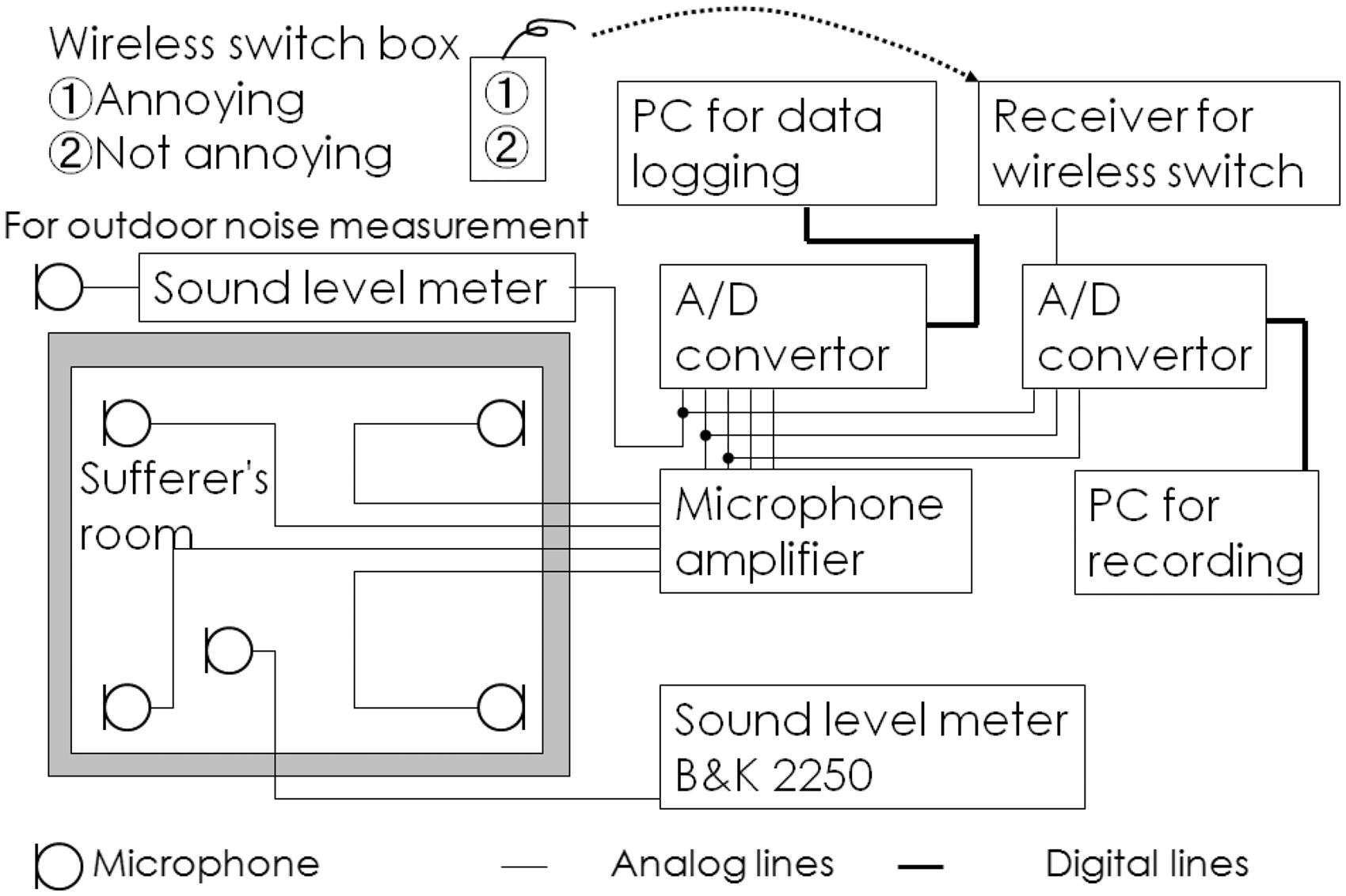
On-site measurement system of the environmental noise with low-frequency components and the response of a complainant.

The acoustical measurement part of the system consists of four microphones (B&K 4190) for the interior noise measurement that are connected to a four channel microphone amplifier (B&K NEXSUS), a microphone to capture the outdoor noise beside the house (RION NA21 class II sound level meter capable down to 20 Hz), and an eight-channel A/D converter with PC interface and an FFT for 1/3 octave band analysis (Ono Sokki DS-2000).

During measurements, two class I sound level meters capable of measurements down to 3 Hz (B&K 2250) were also used to increase the number of measurement points and to confirm the accuracy of the measurement results from the other microphones.

Software

All of the microphone inputs were acquired by the PC (Personal Computer; CPU: Intel Q6600, OS: Windows XP) via the A/D converter (Ono Sokki DS-2000). The other PC and audio interfaces (RME Fireface 800) were used for recording the signals captured by the microphones. The software performs FFT analysis and 1/3 octave band analysis of up to eight channels while measurements were carried out. All of the data that make up a set of measurements (six channels in the PC, the class I sound level meters (B&K 2250), and the complainant's response) were stored as a text file that is used as an input to a prepared Microsoft Excel file. The Excel file was used to analyze the data and prepare graphs suitable for the presentation to the complainant just after the measurements are taken. The detailed contents of the automated analysis functions will be presented in the following section. In the future, we are planning to replace the functions being done by Excel with a new software package that can be used by officers of local governments.

Measurement of the SPL and the complainant’s response

The measurement of the noise and the complainant’s subjective response was carried out in the living room of a house. The complainants declared that they had been suffering from a LFN, which was thought to be generated by outdoor air conditioning units (compressors) located at an adjacent house. The measurements were carried out at his house over a 24 h time span. The analysis used in this example covered a 2 h period in the night during which he seriously responded to the noise (1:00 AM–3:00 AM). Because it is often difficult to determine the time when the suspicious noise source can be observed, long-term measurements more than a day in length are required. Noises were measured on the center position (position “A”) of the bedroom, where the complainant most often feels annoyed and outside close to the suspicious noise source. In addition, the complainant’s detection of the suspected noise was also measured in the center of the room using the switch box of subjective response.

Figure 2 presents the 1/3 octave band level measured in the bedroom of a complainant’s house and outside. The averaged SPL in the 1/3 octave band was calculated while the complainant’s response button was on. Figure 2 also presents the reference value which is published by the Ministry of the Environment in Japan and entitled “The reference values for complainants about mental and physical discomfort (MOE reference level)”.²² The reference value is a useful tool to judge whether or not the sound environment is providing discomfort to the occupants. Figure 2 indicates that, on average, there were no LFN components above the MOE reference level, nor were any above the hearing threshold level, in the band below 100 Hz during the measurement period. The A-weighted equivalent sound level (Leq) was 32 dB at position “A” of the bedroom and 40 dB at the “Outdoor” position, both of which are less than the reference value of the Japanese environmental regulations for residential areas. Since complainer was suffering from the noise with a lower level than regulation, he thought that the low frequency of the noise could be a major problem causing annoyance.

Figure 2.

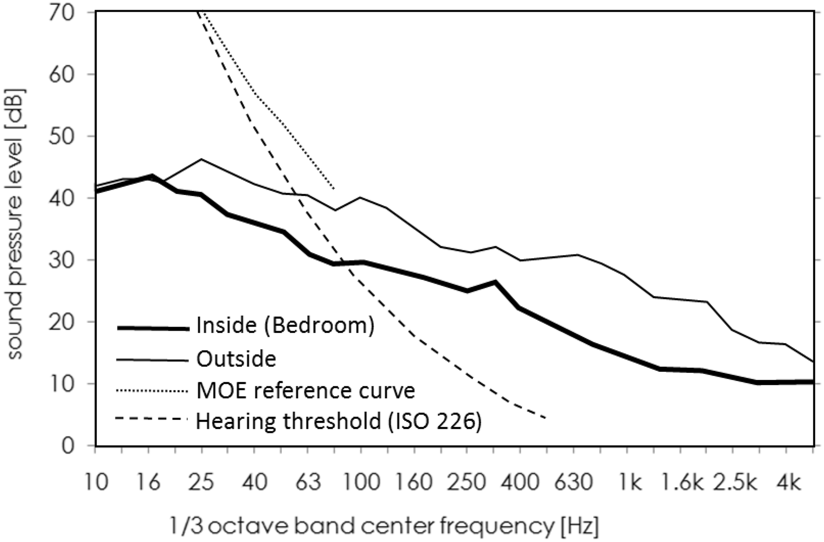
Leq of each 1/3 octave band measured at the sufferer’s house. MOE reference curve and hearing threshold (ISO 226) are also presented.

Procedure of automated analysis

Analysis flow

Figure 3 presents a flow chart of the procedure used to analyze the measured data and the complainant’s response in order to determine the major SPL spectrum band and dominant frequency causing annoyance. This procedure was performed by recording the equivalent continuous SPLs in each 1/3 octave band along with the complainant’s response (“1,” “response” or “0,” “no response”) every 10 s. The noise measurements were divided into “response” and “no response” categories, and then compared. First, the difference between the “response” and the “no response” SPL data and then the frequency distribution of the response and no response data were calculated. Next, the SPL of each frequency band was compared with the reference value from the MOE (Japanese Ministry of the Environment)³³ and 10 phon curve from the equal loudness level contours.³⁷ In order to select the major frequency spectrum that is causing the complaint, the percentage of data exceeding the criteria and the corresponding response data was calculated for each SPL measurement across the spectrum. Then, the percentage of response data that corresponded to measurements higher than the criteria, the differences in the SPL when the complainant's response changed, and the point-biserial correlation between the SPL and the responses in each frequency band at each data point were analyzed to determine the dominant frequency that is causing complaint.

Figure 3.

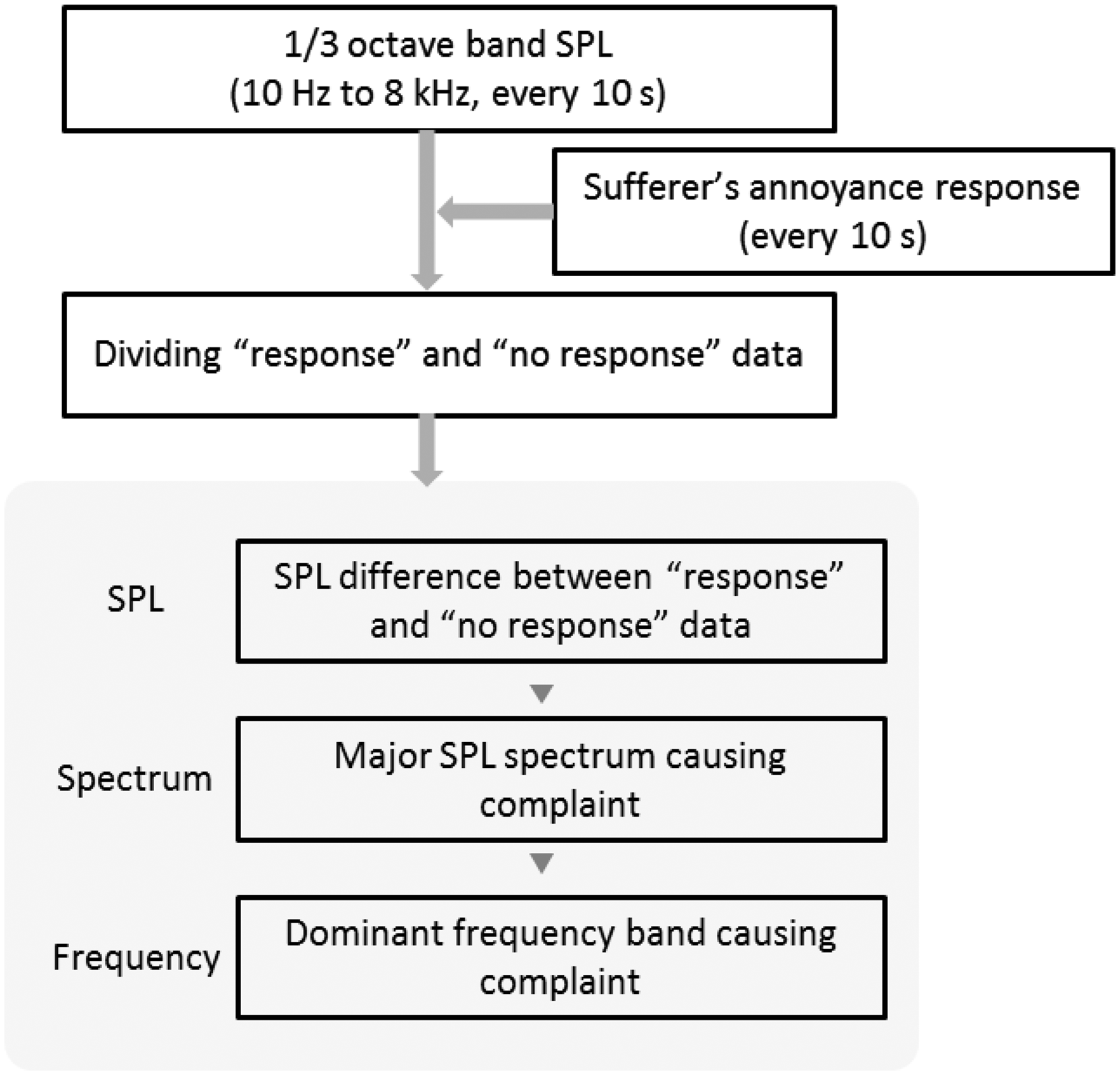
Flow chart for the analysis of the noise and the complainant’s response.

SPL difference between the “response” and “no response” data

The data gathered by tracking the annoyance response from a complainant were divided into “response” data and “no response” data. Figure 4 presents the mean SPL difference in each band while taking into account the “response” and “no response” data. The positive difference means that there was more “response” data than the “no response” data. The difference between the “response” and “no response” data in the 63 Hz and 315 Hz band was largest about 2 dB at position “A” of the bedroom. This was the position where the complainant declared that he had been annoyed by the LFN.

Figure 4.

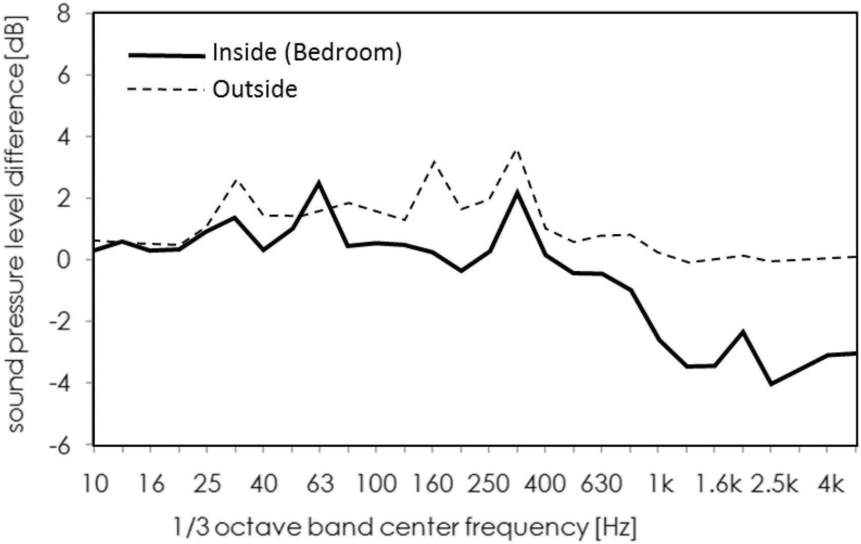
Average difference of the SPL in each 1/3 octave band in the “response” and “no response” period.

Major SPL spectrum causing complaint

In order to judge the impact of the LFN on the annoyance level, it is important to measure not only the variation in the level of the LFN but also the relationship between the lower frequency and higher frequency components. This relationship can be observed in the SPL spectrum in 1/3 octave bands. It is necessary to find out which portion of the SPL spectrum is causing most of the complainant’s annoyance. Because there is a wide frequency range in the SPL spectrum data when it is measured every 10 s, it is also important to have the lower and higher frequency-related criteria to guide the classification of the data. The criteria used in the present study were based on two references: the MOE reference level³³ for the low-frequency range between 10 Hz and 80 Hz and 10 phon curve from the equal loudness level contours³⁷ for the middle- and high-frequency range between 100 Hz and 10 kHz. The 10 phon curve was selected because it is easily connected to the MOE reference level at 80 Hz. The criteria can be changed depending on the measured noise data for individual measurements, as shown in Figure 5. For example, when the measured SPL is quite high, it is possible to use 20 or 30 phon curve of the equal loudness level contours for classification, instead of 10 phon curve.

Figure 5.

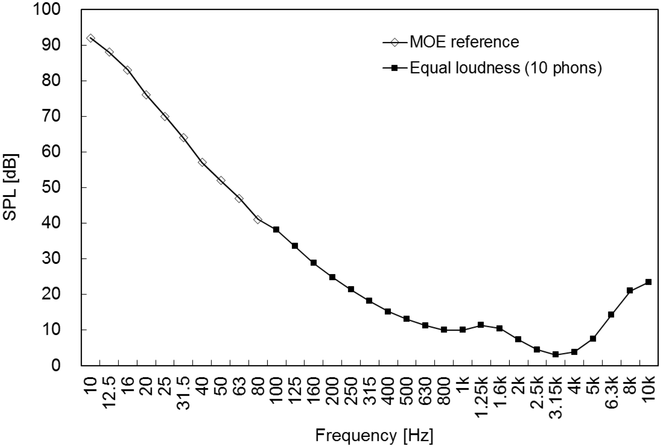
Reference curves for classifying the measured interior noise; MOE in the range from 10 to 80 Hz and 10 phons curve in the range from 100 to 10k Hz.

Figure 6 presents an example of the classification of the SPL spectrum measured in the complainant’s house. All of the example data used in this paper were measured in or around the same house. The SPL spectrum was described using 0–1 bits in six frequency ranges ([10–16 Hz], [20–40 Hz], [50–80 Hz], [100–160 Hz], [200–630 Hz], and [800–5000 Hz]). The frequency range was first divided into three ranges: low (below 160 Hz), middle (200–630 Hz), and high (over 800 Hz). The low-frequency range was then divided into four additional ranges for detailed investigation. The SPL was measured every 10 s and compared to the value of the criterion for each frequency band. If the SPL in a frequency band exceeded the criterion in each frequency range, the output was marked as “1.” If the criterion was not exceeded, the output was marked as “0.” This procedure was used for all the six frequency ranges. Using this method, a total of 64 (2 to the 6th power) SPL spectrum types, based on the results in each frequency range, were classified (e.g., 111111, 111110, 111101, …, 000010, 000001, 000000). Next, the data were again divided into “response” (“1”) and “no response” (“0”) categories on the basis of the response data measured every 10 s. Finally, the percentage of the complainant’s responses (signaling the detection of an annoying sound) to each SPL spectrum type was calculated. The percentage was calculated by dividing the number of “response” data points by the frequency of occurrence of each noise type.

Figure 6.

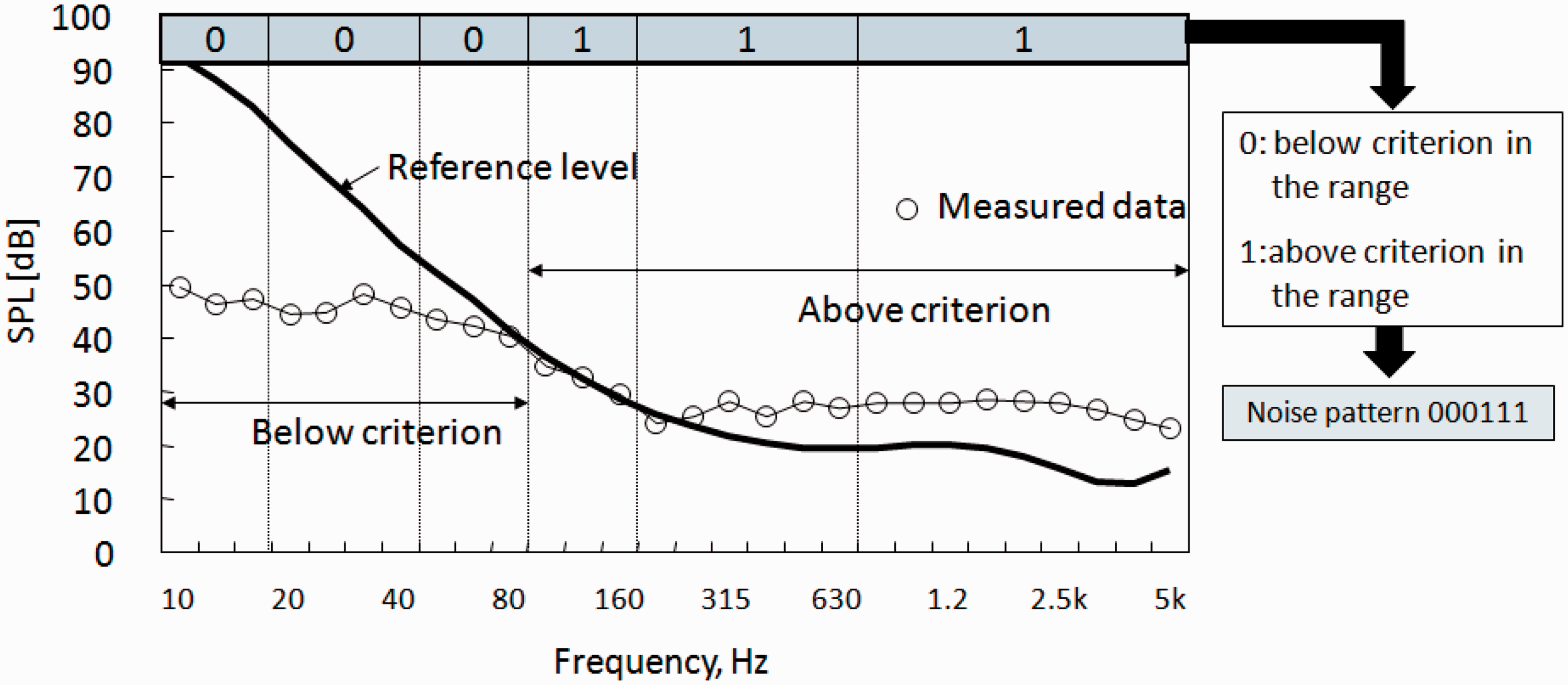
Example classification of the SPL spectrum.

Figure 7 shows an example of the classification of the SPL spectrum and the percentage of each SPL spectrum type to which the complainant responded. Data that had a frequency of occurrence less than 0.5% were excluded in Figure 7, because that data might be related to a temporary sound that happened by accident, such as the complainant’s movement. Figure 7 shows only four significant frequency spectra (001111, 001011, 000111, 000011), which means the lower frequency range than 40 Hz did not have either a high SPL or a high percentage of “response” data. This example suggests that higher frequency components have the largest effect on the annoyance level. All SPL spectrum bands with a high percentage of “response” data also included a portion of the middle and high-frequency range ([200–630 Hz] and [800–5000 Hz], XXXX11 in 0–1 bit). In particular, the spectrum denoted “000011” showed not only the highest percentage of occurrence (84%) but also a high percentage of “response” data. Therefore, this shows that the noise properties in the 200–5000 Hz range are expected to cause most of the annoyance complaints. This expectation is made clear in Figure 8. Figure 8 shows the mean SPL spectrum over all data pieces for each major SPL spectrum type defined in Figure 7. It was revealed that the noise that dominated SPL spectrum bands, as shown in Figure 8, and especially the peak in the 315 Hz band, had great influence on the complainant's response.

Figure 7.

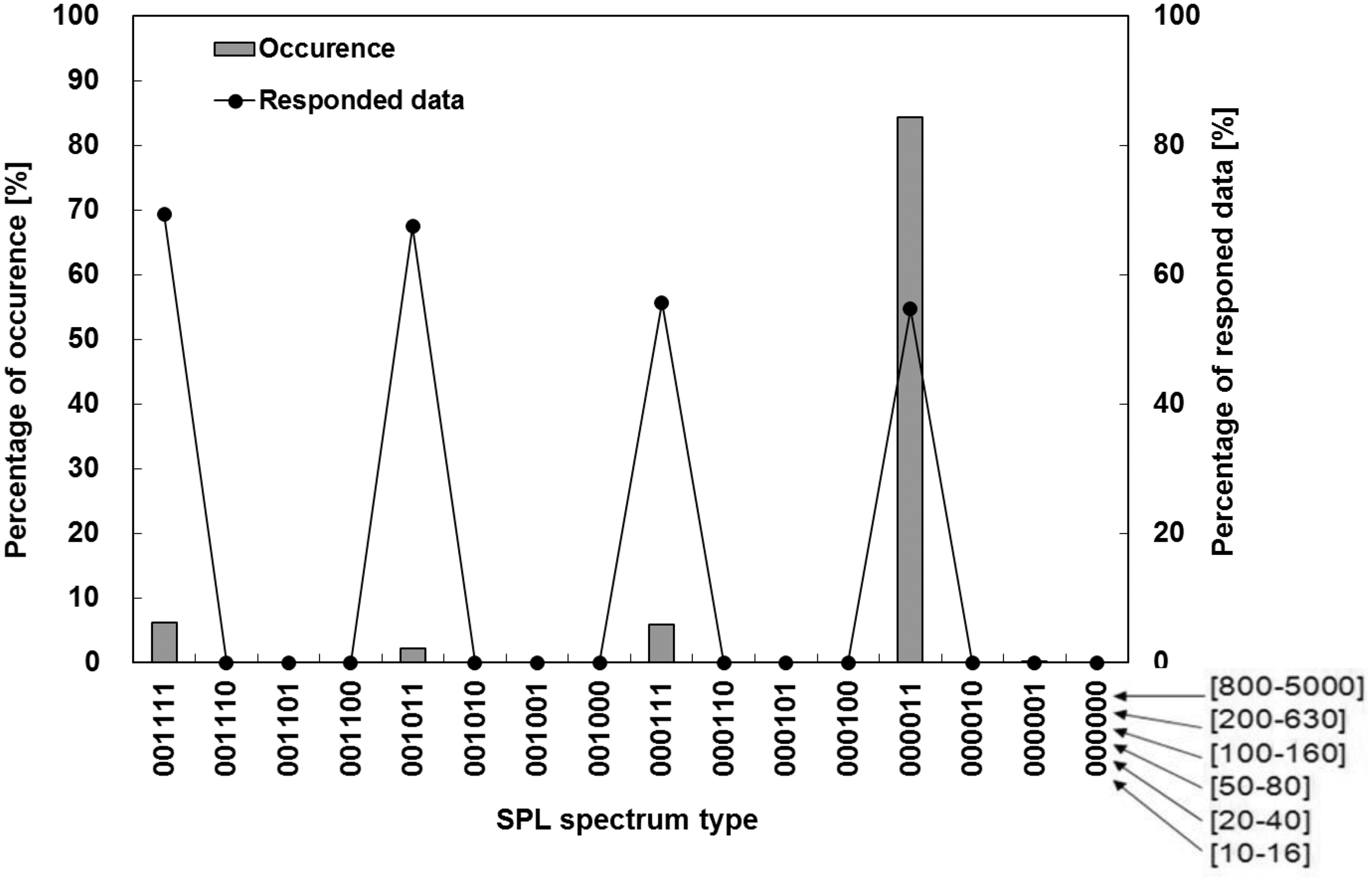
Example classification of the SPL spectrum; frequency (bar) and percentage (line and marks) of SPL spectrum types to which the complainant responded.

Figure 8.

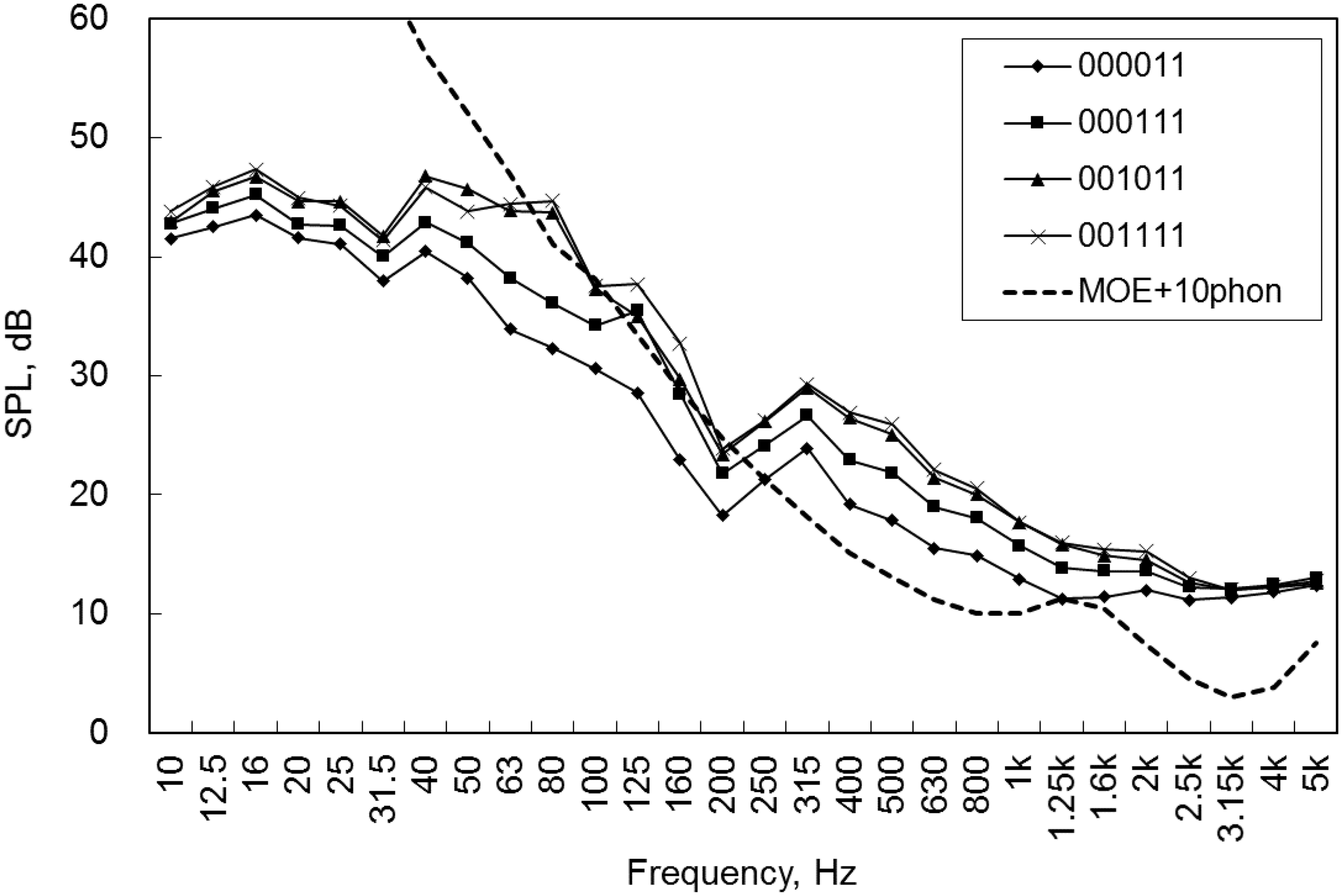
Mean SPL spectrums over all data pieces for each major SPL spectrum type defined in Figure 9.

Dominant frequency band causing complaint

Percentage of “response” data of data exceeding criteria

In the previous chapter, as a result of the division of the spectrum into frequency bands, all data points were divided into four categories [“response,” effective], [“no response,” effective], [“response,” non-effective], and [“no response,” non-effective] corresponding to [1,1], [0,1], [1,0], and [0,0] in 0–1 bits, respectively. Here, ‘effective' means that sound pressure level in each octave band exceeds the reference value of criteria. Figure 9 presents an example of the percentage of “response” data exceeding the criterion in each frequency band. This means the percentage of “response” data ([“response,” effective] in [1,1] in 0–1 bits) in all of data exceeding the criterion (both [“response,” effective] and [“no response,” effective], both [1,1] and [0,1] in 0–1 bits). Figure 9 clearly shows that the complainant responded to 90% of the data that was above the criteria in the 315 Hz band. This indicated that the noise in the 315 Hz band caused most of the complainant’s annoyance.

Figure 9.

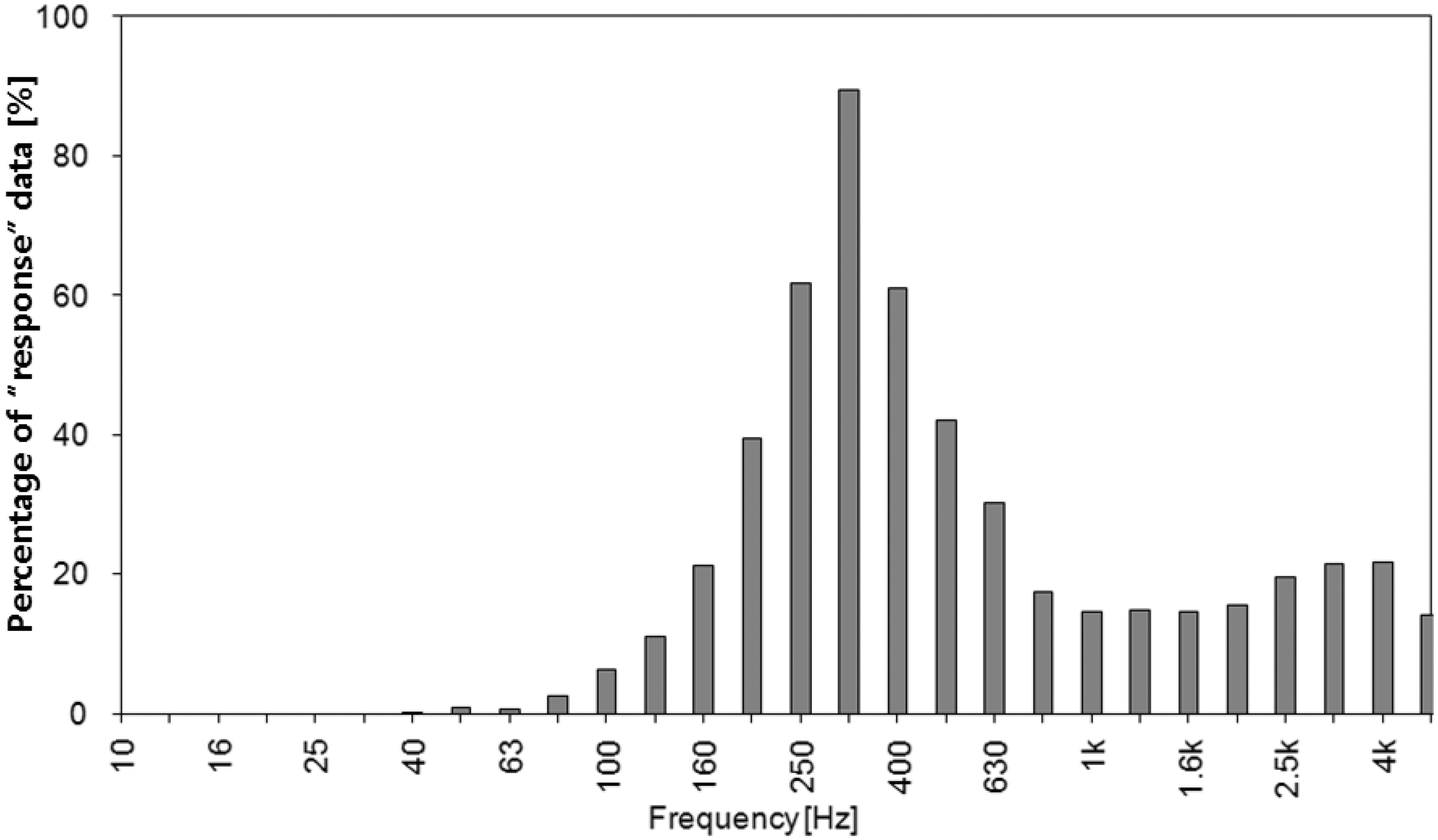
Percentage of the “response” data that exceeded the criteria.

Difference in the SPL between the “response” and “no response” data when the complainant’s response changed

This section describes the method used to investigate the difference in the SPL in each frequency band between the “response” and “no response” data when the complainant’s response changed. It is assumed that the frequency band showing the largest difference might be the most significant frequency band causing annoyance, because people detect the noise more easily when there is a large variation in the SPL. Figure 10 presents the method used to select the applicable portions of the “response” and “no response” data. Because complainant’s response might follow the starting and stopping of the noise, the 30 s period after the beginning and end of the complainant’s response was selected as the “response” and “no response” data, respectively.

Figure 10.

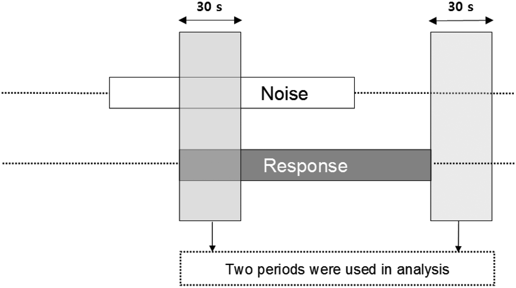
Selection of periods used for the analysis.

Figure 11 presents an example of the mean SPL difference between the “response” and “no response” data when the complainant’s response changed. Figure 11 shows that the 31.5, 63, and 315 Hz bands are related to the annoyance level, and the 1 kHz and above bands are not related to the annoyance level.

Figure 11.

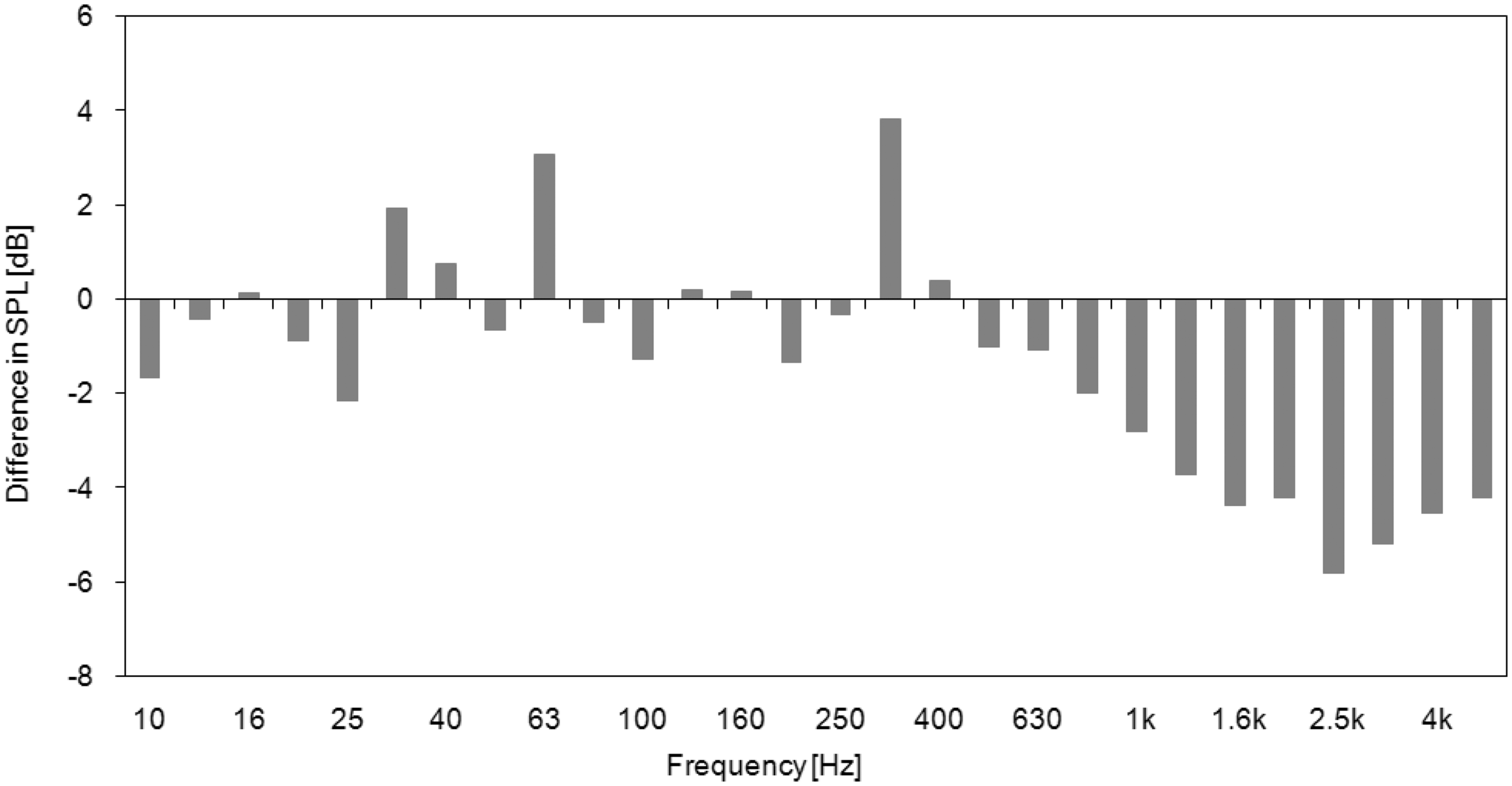
Difference in the sound pressure level between the “response” and “no response” data.

Point-biserial correlation between the SPL and the complainant’s responses

The point-biserial correlation coefficient between the SPL in each frequency band and the complainant’s response was also investigated. The point-biserial correlation coefficient was used because the complainant’s response data are made up of dichotomous variables (“response” or “no response” data) in the present study. However, if the complainant’s response was measured on rating scale, such as “not at all, somewhat, significantly, or extremely annoyed or heard,” Pearson’s correlation coefficient could be also used. The calculation method used to obtain the point-biserial correlation coefficient is exactly the same as the method used to obtain Pearson’s correlation coefficient.

Figure 12 presents the point-biserial correlation coefficient between the 1/3 octave band sound SPL and the complainant’s response. The 315 Hz band has the highest correlation coefficient and is expected to be the dominant frequency. The 31.5 Hz and 63 Hz bands in the low-frequency region are more highly correlated with the complainant’s response.

Figure 12.

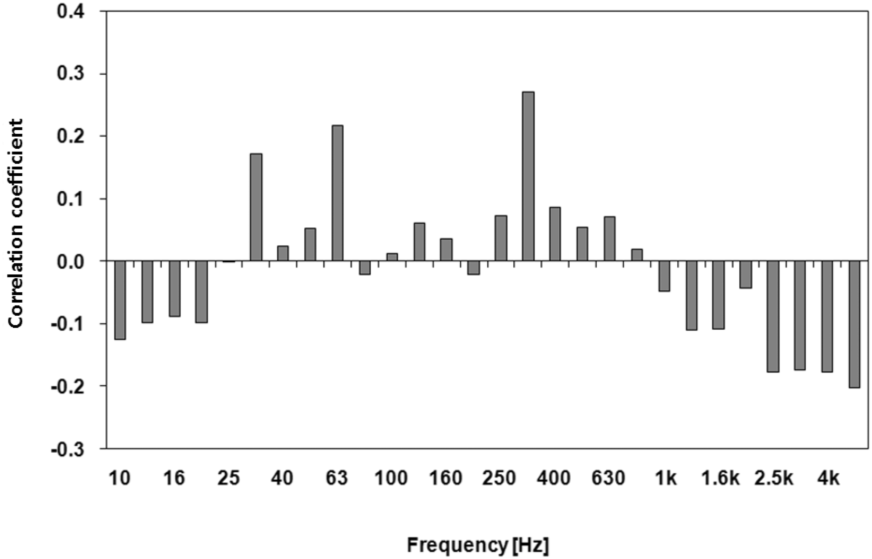
Correlation coefficient between the sound pressure level in each band and the complainant’s response.

Summary of automated analysis

The automated analysis for the example data in the present paper suggests that: (1) the SPL spectrum showing high percentage of “response” data always includes components between 200 and 630 Hz (Figure 7), (2) the SPL in the 315 Hz band is highly correlated with the complainant’s response (Figure 9), (3) the “response” data in the 31.5, 63, and 315 Hz bands have much higher SPLs than the “no response” data (Figure 11), and (4) the SPL in the 315 Hz is most associated with the annoyance response (Figure 12). All of these results indicate that the 315 Hz band is a candidate suspected of causing annoyance.

Discussions

Potential of the present system

Some associations between the exposure to the LFN and the annoyance and health effects were suggested in many studies,^1–8 but no reliable indicator of the annoyance and health effects due to the LFN was found. The A-weighted equivalent sound pressure level (L_Aeq) underestimates the influence of the LFN, and the difference between the C- and A-weighted equivalent level (L_C-A),¹⁷ criteria in the SPL in a 1/3 octave band^18–23 and the normal hearing threshold⁴ was not perfect to estimate clearly the annoyance from the LFN. This difficulty may be due to the two facts. One is that when a complaint from the noise is raised and L_Aeq as usual indicator is below the regulation or criteria, it is suspected that the LFN is the biggest problem for their annoyance. However, in many cases, frequency components causing annoyance are middle and high frequencies, and not low-frequency range. Another fact is because annoyance due to the LFN is not clearly estimated using the solitary regulation with L_Aeq and L_C-A or criteria because perception on the LFN varies with people’s psychological and physiological characteristics.

Our measurement and analysis system can be a useful tool to investigate whether the noise complainant is affected by low-frequency components. Therefore, the present system can be also used to identify people annoyance from other noise sources exposure. For the further discussion, additional data were taken from the noise and subjective response measurements of two houses (A and B), where residents are believed to suffer from the LFN. Measurements method was same as former part, and only data in the center position were used in the discussion. Figure 13 shows that percentage of the “response” data that exceeded the criteria in additional measurements using our suggested analysis system in two dwellings. As shown in House A of Figure 13, the dominant frequency causing complainant’s annoyance is the 40 Hz band in the low-frequency range. On the other hand, in House B of Figure 13, it is somewhat difficult to determine the dominant frequency, but middle frequency band is thought to be that.

Figure 13.

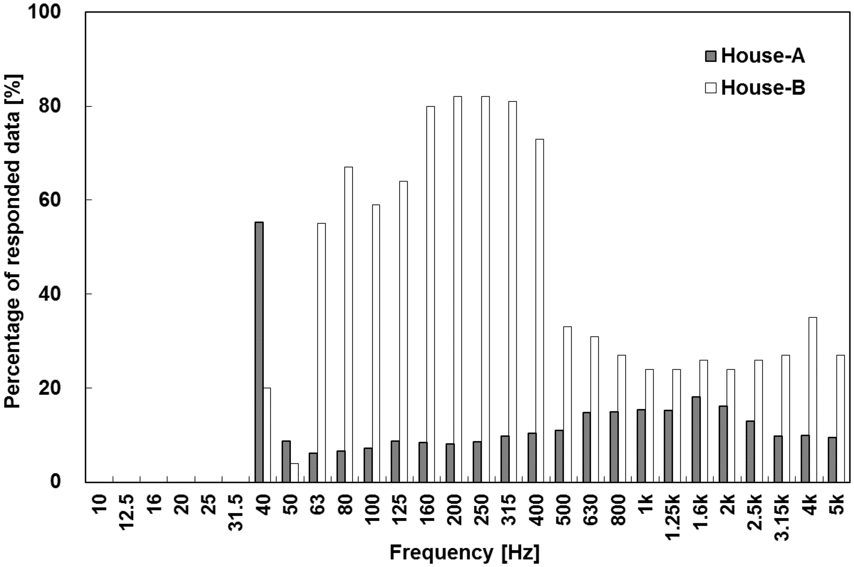
Percentage of the “response” data that exceeded the criteria in additional measurements using our suggested analysis system in two dwellings.

The present system also provides the field measurements and analysis to be oriented towards the individual complainant’s response. Thus, associations between the noise and the people’s responses can be easily found even in field. The most dominant frequency band and major SPL spectrum type causing complaint was determined through the on-site measurement and automated analysis system. The results collected by the present system can be explained more easily and convincingly to the complainant, because the results are quantified based on individual response data. The results include the percentage of data exceeding the criteria, the “response” data for each SPL spectrum band, the percentage of “response” data exceeding the criteria, the differences in the SPL when the response changed, and the point-biserial correlation between the SPL and the responses.

Limitations and precautions

The present system measuring both the noise and the subjective response has some limitations and precautions when it is used in the field as followings: measuring subjective response, background and man-made noise, criteria, and period for measurement.

This system is oriented towards the complainant’s response, and therefore, it is very important to measure variations in the response data. It is desirable that the complainant always be ready to determine their response to the target noise because incorrect complainant responses lead to poor and inaccurate results. In the specific case where the complainant always hears the target sound and is in constant pain, it is only possible to classify the SPL spectrum on the basis of the criteria because there is no variation in the complainant’s response.

For more accurate analysis, all temporal background noise and the noise caused by the complainant should be removed. In the present study, datum whose occurrence frequency is less than 0.5% of all data was excluded from the analysis because the data may have been related to a temporary noise that happened by accident, such as movement by the complainant. The value used as the criteria for excluding data can be varied depending on the noise environment.

Some of the results gathered using the present system depend on various criteria, including the hearing threshold, loudness, the reference value in the 1/3 octave band, etc. As shown in Figure 5, these criteria can be changed depending on the individual noise data measured in different fields. The preferable criteria in the present system are to make more classifications of SPL spectrum types and to gather more variations in the complainant’s response for more detailed analysis of the properties of the noise and the complainant's responses to that noise.

In this study, the noise measurement was conducted every 10 s and the average SPL was then calculated. The average SPL for 10 s is suitable for continuous sound but not for the pulsing noise and external noise events. Therefore, an appropriate time interval for calculating the average SPL should be considered in the case of discontinuous sound.

Conclusions

In the present study, an on-site simultaneous measurement and assessment system was developed for monitoring both the LFN and a complainant’s response to the LFN over a long period. The present paper described an automated post-processing method for the noise measurement and analysis that can detect major SPL spectra and frequency bands that are causing noise complainant’s annoyance. This system can be used as a tool to check whether a noise complainant is affected by low-frequency components. The system can be also applied to all kinds of indoor noises that are suspected to cause annoyance to the occupants.

Footnotes

Acknowledgment

This paper was based on a proceeding paper given at the 13th International Conference on Low Frequency Noise and Vibration and Its Control in Tokyo on October 2008.

Declaration of conflicting interests

The author(s) declared no potential conflicts of interest with respect to the research, authorship, and/or publication of this article.

Funding

The author(s) disclosed receipt of the following financial support for the research, authorship, and/or publication of this article: This work was supported by the program of “Environmental Research in Japan,” which was funded by the Ministry of Environment, Japan, in 2006–2009 and partially supported by the National Research Foundation of Korea (NRF) grant funded by the Korean government (MSIP) (no. 2016R1A2B4015579).

References

Baliatsas

van Kamp

van Poll

et al . Health effects from low-frequency noise and infrasound in the general population: Is it time to listen? A systematic review of observational studies. Sci Total Environ 2016; 557–558: 163–169.

Chang

Beelen

et al . Road traffic noise frequency and prevalent hypertension in Taichung, Taiwan: a cross-sectional study. Environ Health 2014; 13: 37.

Dzhambov

Dimitrova

Neighborhood noise pollution as a determinant of displaced aggression: a pilot study. Noise Health 2014; 16: 95.

Fidell

Pearsons

Silvati

et al . Relationship between low-frequency aircraft noise and annoyance due to rattle and vibration. J Acoust Soc Am 2002; 111: 1743–1750.

Magari

Smith

Schiff

et al . Evaluation of community response to wind turbine-related noise in Western New York State. Noise Health 2014; 16: 228.

Niven

Fletcher

Pickering

CAC

et al . Building sickness syndrome in healthy and unhealthy buildings: an epidemiological and environmental assessment with cluster analysis. Occup Environ Med 2000; 57: 627–634.

PerssonWaye

Rylander

The prevalence of annoyance and effects after longterm exposure to low-frequency noise. J Sound Vib 2001; 240: 483–497.

PerssonWaye

Bengtsson

Agge

et al . A descriptive cross-sectional study of annoyance from low frequency noise installations in an urban environment. Noise Health 2003; 5: 35–46.

Ascari

Licitra

Teti

et al . Low frequency noise impact from road traffic according to different noise prediction methods. Sci Total Environ 2015; 505: 658–669.

10.

Caniato

Bettarello

Schmid

et al . Assessment criterion for indoor noise disturbance in the presence of low frequency sources. Appl Acoust 2016; 113: 22–33.

11.

G-Q

Zhou

X-X

Chen

X-W.

Annoyance response to low frequency noise with tonal components: a case study on transformer noise. Appl Acoust 2015; 91: 40–46.

12.

Leventhall

A review of published research on low frequency noise and vibration. Contract ref. EPG 1/2/50, Department for Environment, Food and Rural Affairs, London, UK, 2003.

13.

Mirowska

Evaluation of low-frequency noise in dwellings. New Polish recommendations. J Low Freq Noise Vib Active Contr 2001; 20: 67–74.

14.

Jabben

Verheijen

Options for assessment and regulation of low frequency noise. J Low Freq Noise Vib Active Contr 2012; 31: 225–238.

15.

ISO 389-7: Acoustics – reference zero for the calibration of audiometric equipment – Part 7: reference threshold of hearing under free-field and diffuse-field listening conditions, International Standard ISO 389-7:2005, International Organization for Standardization, Geneva, Switzerland, 2005.

16.

Robinson

Dadson

MA.

A re-determination of the equal-loudness relations for pure tones. Br J Appl Phys 1956; 7: 166–181.

17.

Møller

Pedersen

CS.

Hearing at low and infrasonic frequencies. Noise Health 2004; 6: 37–57.

18.

Watanabe

Moller

Low frequency hearing thresholds in pressure field and free field. J Low Freq Noise Vib Active Contr 1990; 9: 106–115.

19.

Moorhouse

Waddington

Adams

MD.

A procedure for the assessment of low frequency noise complaints. J Acoust Soc Am 2009; 126: 1131–1141.

20.

Watanabe

Yamada

Study on perception of complex low frequency tones. J Low Freq Noise Vib Active Contr 2002; 21: 123–130.

21.

Drexl

Otto

Wiegrebe

et al . Low-frequency sound exposure causes reversible long-term changes of cochlear transfer characteristics. Hear Res 2016; 332: 87–94.

22.

Pedersen

Møller

Waye

KP.

A detailed study of low-frequency noise complaints. J Low Freq Noise Vib Active Contr 2008; 27: 1–33.

23.

Benton

The central role of interpersonal conflict in low frequency noise annoyance. J Low Freq Noise Vib Active Contr 2007; 26: 1–14.

24.

Licitra

Fredianelli

Petri

et al . Annoyance evaluation due to overall railway noise and vibration in Pisa urban areas. Sci Total Environ 2016; 568: 1315–1325.

25.

Moorhouse

Waddington

Adams

Proposed criteria for the assessment of low frequency noise disturbance. Research project report, DEFRA NANR45, Acoustics Research Centre, Salford University, UK, 2005.

26.

Waddington

Moorhouse

Adams

Field measurements in the development of methods for the assessment of low frequency noise. J Low Freq Noise Vib Active Contr 2007; 26: 155–164.

27.

Yamada

Inukai

Takagi

et al . Case studies of field measurements of low frequency sound and complaints by a non profit organization for supporting noise, vibration and low frequency noise complainants in Japan. J Low Freq Noise Vib Active Contr 2012; 31: 257–266.

28.

Shehap

Shawky

El-Basheer

TM.

Study and assessment of low frequency noise in occupational settings. Arch Acoust Q 2016; 41: 151–160.

29.

Jakobsen

Danish guidelines on environmental low frequency noise, infrasound and vibration. J Low Freq Noise Vib Active Contr 2001; 20: 141–148.

30.

DIN 45680. Messung und bewertung tieffrequenter geräuschimmissionen in der nachbarschaft [Measurement and assessment of low-frequency noise emissions in the neighbourhood]. Deutches institut für normung, Germany, 1997.

31.

ÖNORM S 5007. Messung und bewertung tieffrequenter geräuschimmissionen in der nachbarschaft [Measurement and assessment of low-frequency noise emissions in the neighbourhood]. Österreichishes normungsinstitut, Austria, 1996.

32.

Nederlandse Stichting Geluidhinder. NSG-Richtlijn laagfrequent geluid [Guidelines for low-frequency noise]. 1–25, Nederlandse stichting geluidhinder, The Netherlands, 1999.

33.

The Ministry of Environment, Government of Japan. Handbook to deal with low frequency noise. Office of Odor, Noise and Vibration, Air Quality Management Division, 2004.

34.

Socialstyrelsen. Buller Inomhus [Low-frequency noise in dwellings]. SOSFS 2005:6 (M) Allmänna råd Socialstyrelsen, Sweden, 2005.

35.

Berg

F.G.P.v.d.

Low frequency sound in dwellings: a case control study. J Low Freq Noise Vib Active Contr 2000; 19: 59–71.

36.

Møller

Lydolf

A questionnaire survey of complaints of infrasound and low-frequency noise. J Low Freq Noise Vib Active Contr 2002; 21: 53–64.

37.

ISO 226: Acoustics – normal equal-loudness-level contours, International Standard, International Standard ISO 226:2003. International Organization for Standardization, Geneva, Switzerland, 2003.

Development of an on-site system for measuring the low-frequency noise and complainant’s responses

Abstract

Keywords

Introduction

Structure of the system

Hardware

Software

Measurement of the SPL and the complainant’s response

Procedure of automated analysis

Analysis flow

SPL difference between the “response” and “no response” data

Major SPL spectrum causing complaint

Dominant frequency band causing complaint

Percentage of “response” data of data exceeding criteria

Difference in the SPL between the “response” and “no response” data when the complainant’s response changed

Point-biserial correlation between the SPL and the complainant’s responses

Summary of automated analysis

Discussions

Potential of the present system

Limitations and precautions

Conclusions

Footnotes

Acknowledgment

Declaration of conflicting interests

Funding

References