Application of machine learning algorithm for the prediction of lupus nephritis using SNP data,polygenic risk score,and electronic health record

Abstract

Background: Lupus nephritis (LN) flares raise the risks of renal failure and mortality in systemic lupus erythematosus (SLE) patients, making risk stratification and individualized care crucial. Our goal was to develop machine learning (ML) models to predict LN flares. Methods: A total of 1546 SLE patients were enrolled from a hospital-based cohort. Electronic health record (EHR), single nucleotide polymorphism (SNP), and polygenic risk score (PRS) were combined to construct ML models. SHapley Additive exPlanation (SHAP) values were calculated to assess each feature’s contribution. Results: Within 5 years, 448 patients developed LN. Of the 686,354 SNPs, 375 were used for PRS computation. The model combining EHR, SNP, and PRS achieved the highest AUROC of 0.9512 and AUPRC of 0.8902 in validation, while the XGB-based hybrid model reached an AUPRC of 0.9021 in testing. The SHAP summary plot highlighted the top 20 features predicting LN flares. Conclusions: This hybrid model combining SNP, PRS, and EHR predicts active LN and requires validation.

Introduction

Lupus nephritis (LN) is commonly seen in 50% of patients with systemic lupus erythematosus (SLE).^1,2 Early detection of LN and timely immunosuppressive treatment could drastically improve the renal outcome. ³ In contrast, severe forms of LN could sustain irreversible renal damage and a higher mortality risk. ⁴ Active nephritic flare in SLE patients contributes to deleterious renal outcomes. ⁵ However, early identification of active LN is challenging. Several risks factors can predict active renal flares,^5–7 including renal pathology. However, an invasive renal biopsy procedure could prove risky in patients with severe LN. Although clinical features have been associated with renal flares, the limited number of analyzed cases and variables prevent the extensive clinical application.^5–7

Machine learning (ML) algorithms have found wide application in facilitating a diagnosis and outcome prediction in SLE.^8–11 In a previous study, an SLE Risk Probability Index using clinical features was proposed to facilitate a diagnosis of SLE. ⁸ In addition, Chen et al. built a prediction model using demographic, immunological, and pathological variables to identify renal flares. ⁹ ML models developed using traditional EHR and novel urine cytokines and chemokines appeared promising for the prediction of renal outcome. ¹¹ Moreover, ML models using histopathological and laboratory variables could forecast therapeutic response to immunosuppressants. ¹⁰ However, previously reported ML models for SLE are mainly based on clinical parameters.^8–11 It is unknown whether an ML algorithm combining clinical and genetic data can predict renal flares in a patient with LN.

The pathophysiology of SLE is not fully elucidated. However, family aggregation and twin cluster suggest a genetic component in the etiopathogenesis of SLE. Polygenic risk scores (PRS) obtained by a weighted calculation of multiple single-nucleotide polymorphisms (SNP) are associated with the age of SLE onset, renal disease, damage accrual, and decreased overall survival.^12,13 Our previous study has established robust ML models for genomic prediction of SLE using genome-wide SNP data. ¹⁴ However, the use of PRS in the ML model to predict LN clinical outcomes has not been elucidated. In this study, we aimed to develop ML models using clinical, laboratory, immunological, genetic data by SNP, and PRS to predict LN flares in SLE patients.^15,16

Materials and methods

Study design and study population

Between June 2019 and August 2021, we conducted a retrospective cohort study of 43,035 participants in a tertiary referral hospital. The data were extracted from a hospital-based cohort as previously described.^14–16 Participants from the initial cohort were excluded according to the following criteria: (1) retained participants diagnosed with SLE; (2) excluded patients without UPCR records or a history of LN; (3) excluded patients without available GWAS data; and (4) included patients who met the outcome definition within 5 years and excluded those with early withdrawal or incomplete data. Following these criteria, a total of 1546 participants diagnosed with SLE and without a history of LN were included in the final analysis. ¹⁷ The detailed patient selection process is presented in Supplemental Figure 1. The study protocol was approved by the Ethics Committee (SF19153A). Each participant provided written informed consent.

Genotyping

SNP genotyping of SLE patients was performed using a version 2 biobank genotyping array (Thermo Fisher Scientific, Inc., Santa Clara, CA, USA).^14,18 The quality control of genotyping was verified by the total call rate and minor allele frequency (MAF) as previously described.^14,18

Extraction of data on clinical features

Data on the clinical parameters were extracted from the electronic health records (EHR). The estimated daily urinary protein was obtained by a spot urine protein-to-creatinine ratio (UPCR). Anti-dsDNA antibody (Anti-dsDNA ab) detection was performed using the enzyme-linked immunosorbent assay (ELISA) method (QUANTA Lite dsDNA, Inova Diagnostics). Complement levels of C3 and C4 were determined by polyethylene glycol-enhanced immunoturbidimetric assay (Siemens Healthineers, Erlangen, Germany).

Comorbidities, including diabetes mellitus (ICD9-CM code 250.00-250.92; ICD10-CM code E08.00-E13.9), hypertension (ICD9-CM code 401.00-404.93; ICD10-CM code I10-I13.2), and hyperlipidemia (ICD9-CM code 272.0-272.4; ICD10-CM code E78.0-E78.5), were categorized by the diagnostic codes at least twice in the outpatient and at least once in the inpatient settings within 6 months of SLE diagnosis.

Outcome definition of LN

The primary outcome was defined as the occurrence of active LN within a 5-years timeframe following the initial diagnosis of SLE. Active LN was characterized by the presence of significant proteinuria, defined as a UPCR≥500 mg/mL. ¹⁹ While renal biopsy remains the gold standard for definitive LN diagnosis, UPCR was chosen as a validated, non-invasive marker of active renal disease that is routinely monitored in clinical practice.

Data preprocessing

For predicting LN within 5 years at the first SLE diagnosis, we used the patient’s clinical information, including demographics, comorbidities, biochemical profiles, and medication records. The index date was defined as the date of first SLE diagnosis for the individual and the outcome date was defined as the first date on which the SLE patient was diagnosed with LN. Baseline biochemical profiles of anti-dsDNA ab, C3, C4, serum creatinine, and the estimated glomerular filtration rate (eGFR; calculated through the Modification of Diet in Renal Disease equation), ²⁰ hemoglobin, white blood cell (WBC), erythrocyte distribution width (EDW), lymphocyte count, and platelets that were measured within the 1 year before and the 1 year after the index date and prior to the outcome date were obtained. Medication records of glucocorticoid and immunosuppressants were collected 6 months before and after the index date and prior to the outcome date. With regard to the processing of missing or invalid values for clinical data, we utilized the KNN imputer (n_neighbors = 2) available in the scikit-learn package. This method was selected due to its ability to leverage observed data patterns to provide contextually relevant imputations, making it particularly suitable for handling clinical datasets with mixed variable types. ²¹ In our study, the KNN imputer demonstrated superior performance during the validation phase, reinforcing its suitability for our analysis. The biochemical profiles were removed if the percentage of missing value was greater than 40%. The quantification of missing values across all variables is presented in Supplemental Table S1. Furthermore, data normalization was adopted to improve the accuracy of ML models. ²² During the model validation phase, we assessed multiple normalization techniques on the default model, including the min-max scaler, standard scaler, and robust scaler. The results indicated a slight advantage of min-max scaling, leading to its selection as the preferred normalization method. Therefore, we normalized the feature to a range of 0–1 for the continuous variables and a binary value for the categorical variables.

Considering the analysis of genome-wide association studies (GWAS), the SNP values were encoded as 0, 1, and 2 based on the minor allele count in accordance with the concept of the additive genetic model. ²³ Missing SNP values were imputed using the mode within the training set, ensuring the preservation of SNP properties, consistency with genotype classifications, and the avoidance of biologically implausible values. To avoid the confounding effects of SNP data, we removed the SNP data that had greater than 30% missing value. ²⁴ Furthermore, we generated the PRS from the candidate SNPs to quantify the individual genetic risk for LN ²⁵ and developed a modified PRS weighted by the p-value (PRSw) that was obtained from the single association test of GWAS. The PRS of individual genetic variant was defined as ²⁶ :

${\text{PRS}}_{ij}={\beta }_j\times SN{P}_{ij}$

(1)

where β _j is the effect size of the j ^th SNP estimated from the Logistic Regression (LR), and SNP _ij is the SNP value of the j ^th SNP on the i ^th individual.

However, traditional polygenic risk scoring methods treat the impact of all SNPs on disease risk as equal, overlooking the varying contributions of individual SNPs to disease susceptibility. ²⁷ Moreover, research has demonstrated that when multiple weakly associated SNPs are considered, linear PRS models perform better at capturing these small effects. ²⁸ To address this, we developed an enhanced linear PRS model, termed PRSw, which is based on the linear relationships between SNPs and assigns weights to each SNP according to its p-value derived from univariate additive logistic regression in GWAS:

${\text{PRSw}}_i={\displaystyle \sum }_{j=1}^m{\beta }_j\times SN{P}_{ij}\times -{\log }_{10}\left(p-valu{e}_j\right)$

(2)

where m denotes the total number of candidate SNPs selected from the association test.

This approach takes into account the cumulative effects of candidate SNPs, enabling more accurate quantification of each SNP’s contribution, ultimately improving overall prediction accuracy. ²⁹ To prevent data leakage and ensure valid model evaluation, preprocessing of clinical and SNP features, such as normalization and missing value imputation, was performed solely on the training set, with the same parameters subsequently applied to the validation and testing sets.

Feature selection

The GWAS analysis is a prescreening tool for the identification of genetic variants that are associated with the outcome between the case and control populations. ³⁰ To avoid the issue of highly dimensional data, the feature selection approach was employed to identify the most relevant SNPs. ³¹ Therefore, we utilized a single association test of LR to scan for the SNPs that were associated with the outcome. These candidate SNPs were extracted based on a p-value <1 × 10^-3 from the following analysis.

As PRS could quantify the effect of an individual SNP on the outcome,^25,29 we adopted a default random forests (RF) model ³¹ to select a best feature combination of SNP data from the encoding scheme by the minor allele count (called SNP 012), the PRS derived by the SNP 012 (called SNP PRS), as well as the PRSw for individual (called SNP PRS + PRSw). Similarly, we adopted a default RF model to select a best feature combination from the clinical-only data, SNP-only data, and features combining the clinical and SNP data (called Clinical + SNP).

After confirming the best feature combination from the analysis mentioned above, a feature selection technique of recursive feature elimination with cross-validation (RFECV) was conducted. ³² We adopted RFECV on a default RF model with 5-fold cross-validation (CV) to identify and exclude features with minimal contribution or those that did not enhance the evaluation metrics. Due to the data imbalance in this study, the binary F1 score was used as the evaluation metric, as it focuses on identifying true positive cases of LN. This choice also reflects a critical clinical concern—false negatives, which represent undiagnosed LN cases, can lead to delayed treatment, disease progression, and worse patient outcomes. Therefore, prioritizing sensitivity to reduce false negatives is essential in this predictive context. This iterative process systematically excluded such features, ensuring the final feature set was refined to optimize the model’s performance. The RFECV process ultimately yielded an optimal set of 55 features, which were consistently applied across the entire modeling pipeline, including training, validation, and testing phases. A detailed list of features excluded through the RFECV process is presented in Supplemental Table S2, while the complete set of selected features is provided in Supplemental Table S5.

In summary, a five-step feature selection process was implemented to enhance data integrity and model performance. Lab features with >40% missing values and SNP features with >30% missing values were first excluded. GWAS analysis was then applied to retain SNPs significantly associated with the outcome (P < 0.001). A random forest model was used to identify the optimal combination of feature types, revealing that integrating clinical and SNP features achieved superior predictive performance. Finally, RFECV was employed to select the most informative features from the combined set for model training.

ML models

In this study, our entire study population consisted of patients diagnosed with SLE. Within this population, we defined two groups for our ML model development: (1) the case group, which included SLE patients who developed LN within 5 years of their SLE diagnosis, as evidenced by UPCR ≥500 mg/dL, and (2) the control group, which included SLE patients who did not develop LN within the 5-years follow-up period (UPCR remained <500 mg/dL). Of the total 1546 SLE patients, 448 patients (29%) developed LN within 5 years (case group), while 1098 patients (71%) did not develop LN (control group).

For predicting which patients would have LN within 5 years from the first SLE diagnosis, we employed five ML models, including LR, RF, Support Vector Machine (SVM), eXtreme Gradient Boosting (XGB), and Light Gradient Boosting Machine (LGBM) to address this binary classification task. Initially, the dataset (n = 1546) was randomly divided into a training set of 80% and a testing set of 20% by using stratification. We further split the training set into a training set of 90% and a validation set of 10% after the data preprocessing, and the validation set was used to select the feature combination that was best for this study. To achieve robust model performance, the hyperparameter optimization with k-fold CV (k = 5) was performed using the package of GridSearchCV in the training set. ³³ This study faced a problem with class imbalance and, therefore, the synthetic minority oversampling technique (SMOTE) was employed to balance the number of the minority class in the training set. Considering the issue of limited data volume in this study, oversampling techniques were more suitable for addressing the data imbalance problem than undersampling. In addition, the technique of TomekLinks was used to remove the unnecessary instances of majority class. Combining TomekLinks with SMOTE could ensure better performance than using one approach individually in the imbalanced dataset.^34,35 To better understand the importance and contribution of features, the SHapley Additive exPlanation (SHAP) approach was deployed to identify the features that were related to the SLE patients with LN. ³² This was an appropriate method to achieve the goal of explainable ML. The SHAP summary plot was adopted to illustrate how the top-20 features influenced the outcome on the best performing ML model. ³⁶

Proposed hybrid approach

In this study, a hybrid approach combining data preprocessing, feature selection, TomekLinks, SMOTE, RFECV, and XGB classifier was proposed to predict SLE patients might develop into LN within 5 years with the issue of imbalanced class. The schematic diagram of the proposed hybrid approach as shown in Figure 1.

Figure 1.

The schematic diagram of the proposed hybrid approach for predicting LN within 5 years from SLE onset.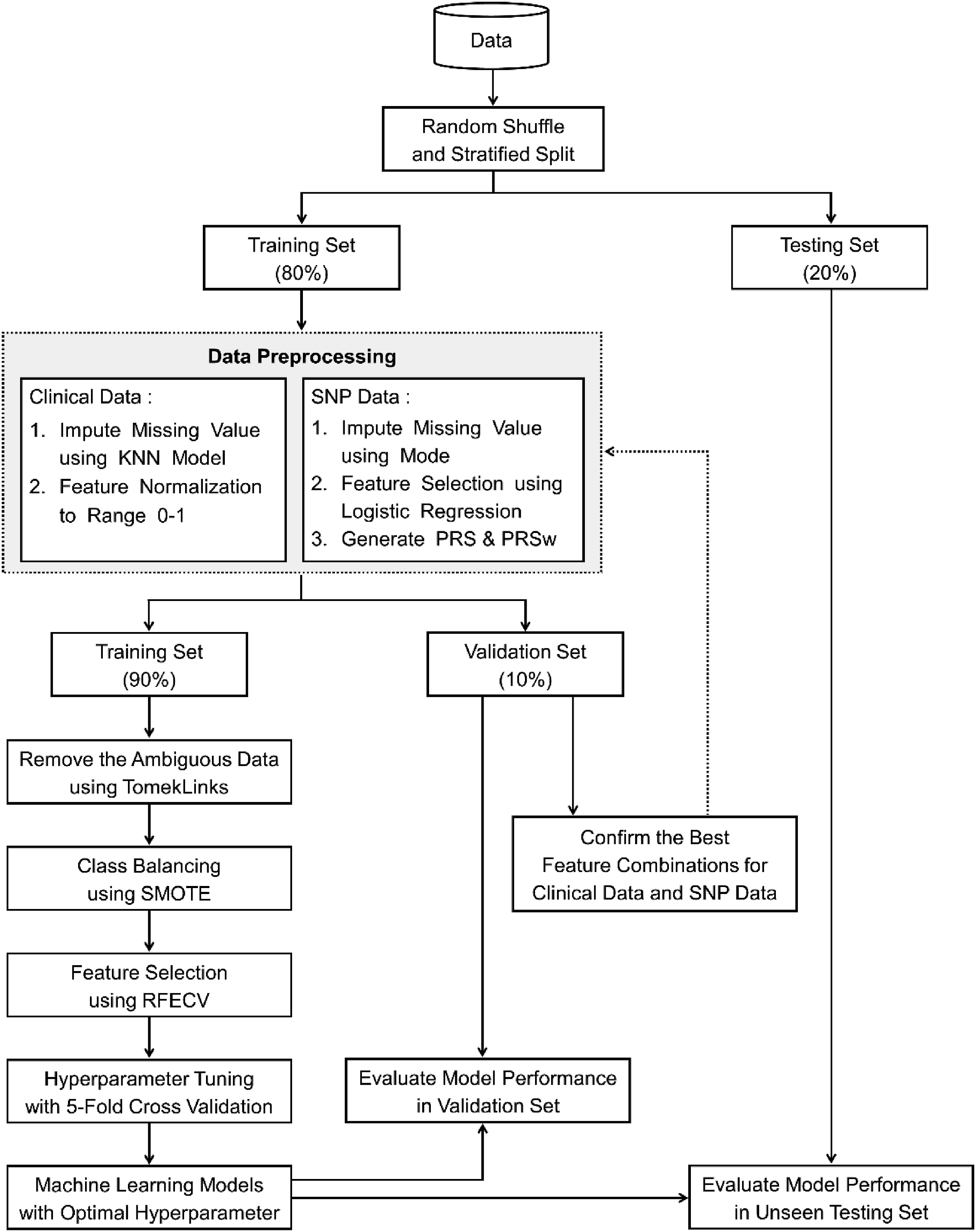

A detailed description is summarized in the following steps:

(1) Random shuffle and stratified splitting of the dataset into the training, validation, and testing sets;

(2) Data preprocessing of clinical and SNP features, where normalization and missing value imputation were performed using only the training set, and the resulting parameters were applied to the validation and testing sets;

(3) Confirm the best feature combinations for clinical data and SNP data based on the RF model in the validation set;

(4) Removal of the ambiguous data using TomekLinks; ambiguous data refers to instances near the decision boundary between the majority and minority classes. These boundary-neighboring pairs were identified and removed to reduce class overlap and improve classification performance, particularly in imbalanced data scenarios;

(5) Class balancing using SMOTE;

(6) Feature selection using RFECV;

(7) Hyperparameter tuning with 5-fold CV;

(8) Training the best machine learning model of XGB with optimal hyperparameter; and

(9) Evaluation model performance based on the proposed hybrid approach in the unseen testing set.

Performance evaluation

To well compare the performance of different ML models, the metrics of accuracy, precision, sensitivity (or recall), specificity, and the F1 score are commonly used to measure the ability for each classifier model. ³⁴ These metrics are presented in Supplemental Table S3.

For the binary classification problem, the area under the receiver operating characteristic curve (AUROC) was widely used to compare the discrimination ability of different ML approaches. ³⁷ However, due to the problem of class imbalance in this study, the appropriate evaluation metric was the area under the precision-recall curve (AUPRC). ³⁴ To robustly examine the performance of the ML models, we adopted the metrics of AUPRC, AUROC, and F1 score as the main evaluation method.^38,39

Statistical analysis

Continuous variables were described as medians with interquartile ranges (IQR), and group comparisons were conducted using the non-parametric Wilcoxon rank-sum test. Categorical variables were presented as counts and percentages, with group comparisons performed using the Chi-square test or Fisher’s exact test when the expected cell frequencies were less than 5. All statistical analyses were two-sided, with a p-value of <0.05 considered indicative of statistical significance. Data preprocessing and statistical analyses were carried out using R software (version 4.4.1), while the development of ML models was performed in Python (version 3.9.7).

Results

Selection of candidate SNPs associated with LN and non-LN

In total, 686,354 imputed SNPs were identified with LN and non-LN using GWAS analysis. As denoted in Figure 2, a p-value threshold of 1 × 10^-5 (red line) was applied to identify significant associations. However, this threshold was found to be relatively stringent given the results of this study. Therefore, a more permissive p-value threshold of 1 × 10^-3 (blue line) was employed, and a total of 375 SNPs were included in the following analysis of feature selection and calculation of PRS. The detailed information of these 375 SNPs is provided in Supplemental Table S4 to facilitate further interpretation of the results.

Figure 2.

Manhattan plot of the GWAS between the LN and non-LN patients. Red and blue lines indicate the p-value thresholds of 1 × 10⁻⁵ and 1 × 10⁻³, respectively.

Baseline characteristics of the study population

We enrolled a total of 1546 SLE patients, of whom 448 (29%) were diagnosed with LN within 5 years of their initial diagnosis, while 1098 (71%) did not develop LN. This distribution highlights a class imbalance within the dataset (Table 1). Compared with the non-LN group, the LN group had a significantly higher proportion of male participants and hypertension. In addition, the values of anti-dsDNA ab, creatinine, WBC, and EDW were significantly higher in the LN group compared with the non-LN group. However, the values of C3, C4, eGFR, hemoglobin, and lymphocyte count were significantly higher in the non-LN group than in the LN group. Patients with LN had a higher likelihood of receiving mycophenolate mofetil and hydroxychloroquine. Furthermore, the median of PRSw in the LN group was significantly higher than the median PRSw in the non-LN group.

Table 1.

Baseline demographic and clinical characteristics of the study population.

Variables	ALL N = 1546	No LN within 5 years N = 1098 (71%)	LN within 5 years N = 448 (29%)	P-value a
Age at first SLE diagnosis (year)	36.3 (26.9, 47.3)	36.3 (27.4, 47.6)	35.8 (26.3, 46.0)	0.199
Male, n (%)	181 (11.7)	109 (9.9)	72 (16.1)	0.001
Comorbidity, n (%)
Diabetes mellitus	47 (3.0)	35 (3.2)	12 (2.7)	0.597
Hypertension	146 (9.4)	71 (6.5)	75 (16.7)	<0.001
Hyperlipidemia	72 (4.7)	44 (4.0)	28 (6.2)	0.058
Biochemical profiles, median (IQR)
Anti-dsDNA ab (WHO unit/ml)	187.9 (51.7, 567.7)	132.8 (42.8, 438.0)	356.7 (86.0, 886.4)	<0.001
C3 (mg/dl)	91.0 (71.3, 110.0)	94.7 (79.6, 110.3)	75.8 (52.0, 104.6)	<0.001
C4 (mg/dl)	17.1 (10.8, 23.8)	17.9 (12.6, 24.1)	14.7 (7.9, 22.4)	<0.001
Creatinine (mg/dL)	0.8 (0.7, 0.9)	0.8 (0.7, 0.9)	0.8 (0.7, 1.1)	<0.001
eGFR (mL/min/1.73 m2)	74.1 (61.3, 88.1)	74.7 (64.5, 87.1)	72.2 (52.3, 91.1)	0.002
Hemoglobin (g/dl)	12.3 (11.1, 13.2)	12.5 (11.6, 13.4)	11.5 (9.9, 12.8)	<0.001
WBC (/mm3)	5900 (4400, 7888)	5771 (4500, 7450)	6480 (4400, 8905)	0.002
EDW	13.7 (13.0, 14.9)	13.6 (12.9, 14.6)	13.8 (13.1, 15.2)	0.005
Lymphocyte count (/mm3)	22.5 (14.3, 30.9)	25.1 (16.7, 32.5)	17.0 (10.0, 26.1)	<0.001
Platelets (/mm3)	223.0 (172.0, 277.0)	221.0 (178.0, 270.0)	226.0 (162.2, 288.4)	0.637
Medication profiles, n (%)
Glucocorticoid	1289 (83.4)	909 (82.8)	380 (84.8)	0.330
Mycophenolate mofetil	162 (10.5)	72 (6.6)	90 (20.1)	<0.001
Cyclophosphamide	174 (11.3)	121 (11.0)	53 (11.8)	0.647
Azathioprine	480 (31.0)	330 (30.1)	150 (33.5)	0.186
Cyclosporin	70 (4.5)	47 (4.3)	23 (5.1)	0.464
Hydroxychloroquine	1354 (87.6)	976 (88.9)	378 (84.4)	0.015
Genomics profiles, median (IQR)
PRSw	20.4 (4.6, 47.3)	12.1 (−0.1, 24.9)	65.7 (49.5, 84.0)	<0.001

^aP-values are calculated by Wilcoxon rank-sum test for continuous variables and Chi-square test (or Fisher’s exact test as appropriate) for categorical variables.

Anti-dsDNA ab: anti-dsDNA antibody; eGFR: estimated glomerular filtration rate; WBC: white blood cell; EDW: erythrocyte distribution width; PRSw: modified PRS weighted by the p-value.

Selecting the best feature combination to classify LN and non-LN patients

First, we attempted to identify the best feature combination for the SNP data in the validation set. We compared model performance based on the genotype value for SNP 012, SNP PRS, and SNP PRS + PRSw based on a default RF model. As depicted in Figure 3(a), the AUROC increased as the feature combinations changed from SNP 012 to SNP PRS, and SNP PRS + PRSw (AUROC: 0.8307, 0.8490, and 0.8996, respectively). Considering the results of Precision-Recall (PR) curve, the AUPRC of SNP PRS + PRSw of 0.8424 was higher than that of the SNP 012 of 0.7037 and the SNP PRS of 0.7312 (Figure 3(b)). Based on the results of Figure 3, we chose the SNP PRS + PRSw as the best feature combination for the SNP data.

Figure 3.

Comparison of model performance among three SNP feature combinations. (a) ROC curve and (b) PR curve.

Moreover, we identified the best feature combination based on the clinical and SNP data. We adopted a default RF model to evaluate the performance among the clinical data, SNP data, and both clinical and SNP data in the validation set. The model performance with both clinical and SNP features had the highest AUROC of 0.9512 and AUPRC of 0.8902 as compared to the clinical or SNP data only (Figures 4A and 4(b)). Therefore, the clinical and SNP (PRS + PRSw) data were utilized to be the final feature combination for the following ML analysis. In total, 397 features were included in the initial analysis, consisting of 21 clinically relevant features, 375 SNP features, and 1 PRS feature. Detailed descriptions of the 21 clinically relevant features and the PRS feature are provided in Table 1, whereas the 375 candidate SNP features are listed in Supplemental Table S4.

Figure 4.

Comparison of model performance among three feature combinations of clinical and SNP data. (a) ROC curve and (b) PR curve.

Comparison of model performance in the validation and testing sets

Table 2 shows the model performance of five ML models in the validation set. Given the class imbalance problem in this study, we focused on the metrics of the F1 score, AUROC, and AUPRC. The AUROC values were all higher than 0.9 for all of models. Compared with the LR model, the RF, XGB, and LGBM models all exhibited better performance with regard to the F1 score and AUPRC. Furthermore, we evaluated model performance for the unseen testing set (Table 3). Similar to the results of Table 2, the models of RF, XGB, and LGBM had significant performance in the F1 score, AUROC, and AUPRC. In particular, the proposed hybrid framework combined the classifier model of XGB could achieve the highest result with AUPRC of 0.9021.

Table 2.

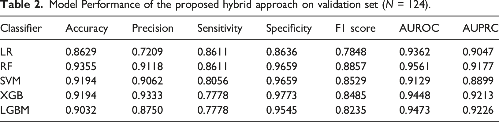
Model Performance of the proposed hybrid approach on validation set (N = 124).

Classifier	Accuracy	Precision	Sensitivity	Specificity	F1 score	AUROC	AUPRC
LR	0.8629	0.7209	0.8611	0.8636	0.7848	0.9362	0.9047
RF	0.9355	0.9118	0.8611	0.9659	0.8857	0.9561	0.9177
SVM	0.9194	0.9062	0.8056	0.9659	0.8529	0.9129	0.8899
XGB	0.9194	0.9333	0.7778	0.9773	0.8485	0.9448	0.9213
LGBM	0.9032	0.8750	0.7778	0.9545	0.8235	0.9473	0.9226

Table 3.

Model Performance of the proposed hybrid approach on testing set (N = 309).

Classifier	Accuracy	Precision	Sensitivity	Specificity	F1 score	AUROC	AUPRC
LR	0.8673	0.7526	0.8111	0.8904	0.7807	0.9070	0.8814
RF	0.8803	0.8046	0.7778	0.9224	0.7910	0.9245	0.8947
SVM	0.8803	0.8442	0.7222	0.9452	0.7784	0.9064	0.8619
XGB	0.9029	0.8571	0.8000	0.9452	0.8276	0.9232	0.9021
LGBM	0.8932	0.8276	0.8000	0.9315	0.8136	0.9164	0.8949

Interpretation of clinical and SNP features for the proposed hybrid approach

To identify the most influential features and improve the interpretability of the proposed hybrid XGB model, Figure 5 illustrates the SHAP summary plot of the top 20 contributors, clearly visualizing the variables with the greatest impact on model performance. As the SHAP value of the features increased, the risk of LN within 5 years increased for SLE patients. For example, an SLE patient has a relatively high risk of LN within 5 years if their PRSw exceeds the median. A more interesting discovery is the result of rs17053102, which showed that an SLE patient had relatively high risk of LN if this SNP was 0/0, because the effect size from LR was −0.38. In contrast, the effect that an SLE patient would develop LN would be protected if this SNP was 1/1.

Figure 5.

SHAP summary plot of the top 20 features of the proposed hybrid framework with XGB model. PRSw: modified PRS weighted by the p-value; Anti-dsDNA ab: anti-dsDNA antibody; EDW: erythrocyte distribution width; WBC: white blood cell.

Discussion

Our study is the first to construct a hybrid framework with the XGB model by using a combination of clinical features, SNP, and PRS to predict the occurrence of active LN in SLE patients. We identified the top genetic and clinical features associated with active LN based on the SHAP summary plot. As the management of LN remains challenging, our model of integrating EHR and genetic variants may provide opportunity to forecast active LN and guide immunosuppressive therapies for high-risk patients.

The integration of our ML models into clinical workflows presents a transformative opportunity to enhance patient care through digital health systems. In the future, the model could be embedded directly into EHR platforms to provide real-time risk assessments for LN development at the point of initial SLE diagnosis. This integration would enable several key clinical applications. First, the automated risk stratification could trigger customized alert systems within the EHR, prompting clinicians to implement preventive strategies for high-risk patients, such as more frequent monitoring of renal function or earlier initiation of immunosuppressants. Second, the system could automatically generate risk-stratified follow-up schedules, with higher-risk patients receiving more frequent screening protocols for early detection of renal involvement. Third, the integration of genetic data with routine clinical parameters in our model demonstrates a practical framework for implementing precision medicine within existing healthcare information systems. Moreover, this approach could serve as a template for similar integration of multi-modal data sources in other conditions. Furthermore, the model’s ability to process both clinical and genetic data in real time could facilitate more informed shared decision-making between clinicians and patients regarding preventive strategies and monitoring intensity. This implementation would represent a significant advance in using health informatics to bridge the gap between complex genomic data and routine clinical care, ultimately improving patient outcomes through early intervention and personalized medicine approaches.

Kruta et al. (2024) achieved notable success in the classification of autoimmune diseases by employing ML models to integrate clinical, laboratory, genomic, immunomic, and metabolomic data. ⁴⁰ Their findings underscore the pivotal role of adopting and integrating patient-derived multi-omics data, which closely aligns with the methodology utilized in the present study. Specifically, our approach leverages EHR data in combination with SNPs and PRS to enhance risk prediction for LN. While the work by Kruta et al. focused on the broader classification of autoimmune diseases, our study uniquely emphasizes LN prediction within SLE patients. Both studies highlight the transformative potential of data integration in addressing complex diseases. Future investigations incorporating multi-omics data akin to the framework proposed by Kruta et al. are anticipated to advance LN risk prediction further and provide critical insights into targeted therapeutic strategies.

A prior study demonstrated a robust prediction power of the 5-years renal flare using clinical data in a biopsy-proved LN cohort. ⁹ However, the aforementioned studies enrolled participants with LN^8,10,11 and aimed to predict adverse outcomes or therapeutic response. Our study, in contrast, attempted to develop a prediction model for LN development. In addition, we included the EHR data, and genetic information for a wide range of SNP levels to PRS from 375 SNPs. Moreover, the SHAP summary plot depicts the top 20 crucial features associated with the development of LN. Interestingly, our data supported the findings of a previous study that EDW was associated with renal relapse, ⁴¹ suggesting that the ML model could identify novel and explicable features in the clinical setting.

Several studies have shown that hybrid models could outperform the existing basic models.^37,42 Owing to the class imbalance problem in this study, the hybrid approach was adopted to improve the predicted performance and the efficiency of clinical diagnosis. Moreover, we hybridized the crucial data preprocessing techniques based on RF and LR models in the feature-selection stage. To overcome the impediment of dimensionality, especially for genetic data, it is necessary to construct a PRS that summarizes the information of the candidate SNPs and utilizes the feature selection of RFECV. ³² Given the complexity of clinical and genetic data, effective handling of missing values is equally critical to ensuring the robustness of the analytical framework. Imputation methods play a crucial role in addressing missing data, yet their effectiveness largely depends on the characteristics of the dataset. Given this variability, selecting an imputation method should be context-driven, considering data properties, disease-specific attributes, and insights derived from validation results. In contrast to the existing work on this topic, our proposed hybrid ML approach showed promising results and a strategy to predict LN flares of SLE patients. Future research could utilize ensemble machine learning models and hybrid frameworks, alongside expanding the sample size. More importantly, given the inherent complexity of kidney-related diseases, beyond applying algorithms that consider variable interactions and the intricate relationships among diseases, incorporating key features that drive disease progression will be pivotal in achieving substantial breakthroughs in research outcomes.

Our data demonstrated that ML models using PRS, SNP and EHRs may robustly predict the development of LN. One previous study showed that PRS from two independent cohorts could predict the SLE phenotype with an AUROC between 0.64 and 0.72. ¹² Another PRS showed an SLE prediction accuracy that ranged from 0.71 to 0.83. ¹³ Our study is the first to demonstrate that ML models using modified PRS in combination with EHR might outperform genetic information alone in SLE patients. The integration of our ML models into clinical workflows presents a transformative opportunity to enhance patient care while reducing economic burden and improving quality of life. By incorporating the model into electronic health record systems, clinicians can access real-time risk assessments for LN development during routine check-ups. This integration could alert physicians to high-risk patients, enabling earlier interventions or more frequent monitoring before irreversible renal damage occurs. Such timely detection and treatment could significantly reduce healthcare costs by preventing progression to end-stage renal disease requiring expensive renal replacement therapies and prolonged hospitalizations. Moreover, this approach can improve patients’ quality of life by minimizing LN flares, reducing symptoms, preserving kidney function, and maintaining patients’ ability to work and participate in daily activities. The personalized risk assessment also allows for optimized resource allocation, ensuring appropriate care intensity based on individual risk profiles while potentially reducing unnecessary interventions for low-risk patients. Furthermore, the model’s predictions could be used to stratify patients in clinical trials, helping to identify those who might benefit most from novel therapies. However, it’s crucial to note that while these models show promise, their implementation would require careful validation in prospective studies. Future research should focus on developing user-friendly interfaces for these models and establishing clear guidelines for their use in clinical decision-making processes.

The present study is the first attempt to build ML model with the hybrid framework. We innovatively adopted RFECV for feature selection by using a combination of EHR and genetic variations of SNP and PRS. In addition, the SHAP analysis provided a mechanical insight of LN. However, several limitations exist. A key limitation of our study is the lack of external validation, particularly in diverse populations. Our study population consisted primarily of Han Chinese individuals, which limits the generalizability of our results to SLE patients of different ethnicities and geographical backgrounds. This limitation underscores the critical need for external validation studies that include multi-ethnic and geographically diverse cohort to ensure the robustness and broad applicability of our ML models across various populations. Lastly, histologic parameters were not included in the analysis. However, our proposed algorithm might facilitate the decision-making for renal biopsy in lupus patients to minimize unnecessary invasive procedures.

Conclusions

This study established robust ML models to predict the development of LN by using a hybrid approach and a combination of the features of EHRs, SNP, and PRS. By using risk stratification and outcome prediction based on clinical and genomic data, our ML model might facilitate precision medicine and artificial intelligence to enable the provision of a better and comprehensive care for SLE patients.

Supplemental Material

Supplemental Material - Application of machine learning algorithm for the prediction of lupus nephritis using SNP data, polygenic risk score, and electronic health record

Supplemental Material for Application of machine learning algorithm for the prediction of lupus nephritis using SNP data, polygenic risk score, and electronic health record by Chih-Wei Chung, Seng-Cho Chou, Chung-Mao Kao, Yen-Ju Chen, Tzu-Hung Hsiao, Yi-Ming Chen in Health Informatics Journal.

Supplemental Material

Supplemental Material - Application of machine learning algorithm for the prediction of lupus nephritis using SNP data, polygenic risk score, and electronic health record

Supplemental Material for Application of machine learning algorithm for the prediction of lupus nephritis using SNP data, polygenic risk score, and electronic health record by Chih-Wei Chung, Seng-Cho Chou, Chung-Mao Kao, Yen-Ju Chen, Tzu-Hung Hsiao, Yi-Ming Chen in Health Informatics Journal.

Supplemental Material

Supplemental Material - Application of machine learning algorithm for the prediction of lupus nephritis using SNP data, polygenic risk score, and electronic health record

Supplemental Material for Application of machine learning algorithm for the prediction of lupus nephritis using SNP data, polygenic risk score, and electronic health record by Chih-Wei Chung, Seng-Cho Chou, Chung-Mao Kao, Yen-Ju Chen, Tzu-Hung Hsiao, Yi-Ming Chen in Health Informatics Journal.