Sage Journals: Discover world-class research

Abstract

Objective: This paper demonstrates a data quality assurance (DQA) process as a means to identify and handle flaws in data, and hence improve the accuracy of an investigation into the prevalence of harmful versus non-harmful/near-miss incident reports in a single NHS acute provider.

Methods: The three-step DQA process consists of an initial univariate data quality analysis, followed by a bivariate missingness analysis, and concluding with the design of appropriate multiple imputation techniques. With data quality established, the acuity and incident data were aggregated and aligned to the Ward-Month level for the period August 2015 to December 2020 inclusive. The final analysis was performed using binary regression, pooling results via Reuben’s Rule.

Results: The application of our three-step quality assurance process was able to detect and correct for common data quality issues. The resulting analysis identified a Ward dependency for the effect of Covid-19 lockdown measures on incident reporting culture which would have been missed without the applied imputation strategy.

Conclusions: Our approach outlines a replicable methodology for understanding and fixing data quality issues in operational data. As daily operational decisions are being guided by data, it is important to leverage appropriate imputation techniques and ensure an optimal decision is reached.

Keywords

data quality missing data routinely collected data

Introduction

Data-driven decision-making has steadily gained pace over the past two decades as electronic storage has become increasingly more affordable, and suites of big data tools have matured to the point of feasibility.¹ Health informatics systems collect vast amounts of data across multiple platforms, much of which is not utilised.² To utilise these data, attention must be paid to data quality in order to determine and guarantee the reliability of findings or intelligence generated. Data quality (DQ) is important to any project that will infer knowledge and is a multi-dimensional construct.³ The importance of DQ in the analysis of large-volume data has been apparent since the 1990s.⁴ It is crucial to establish DQ for data-driven decision-making, and enact strategies to address any potential bias that might be created.

Designing metrics to measure data quality is a nuanced task, as what represents quality and value in one scenario, may be inappropriate in another. A commonly used approach was devised by Pipino et al., taking the form of a checklist comprising sixteen data-quality dimensions³ (see Table 1). Of the sixteen, several are dependent on the skill set, and perspective of the data handler; namely ‘accessibility’, ‘ease of manipulation’, ‘concise’, ‘interpretability’, ‘security’ and ‘understandability’. Of the remaining dimensions, others are dependent on the intended use case; ‘amount of data’, ‘relevancy’ and ‘timeliness’, or are subjective in nature (if we are absent a gold standard to compare with); ‘believability’, ‘free-of-error’, ‘objectivity’, and ‘reputation’. Hence, we are left with three which we can most readily approach with objective measures:

1. Completeness – is data missing, and for what reasons?

2. Consistency – are data and variables represented consistently across the system?

3. Value-added –can the data be reliably used for analysis?

Table 1.

The sixteen dimensions of data quality, adapted from Pipino et al.³

Dimension	Definition - “the extent to which….”
Accessibility	...data is available or retrievable
Appropriate amount of data	...the volume of data is appropriate for a given use case
Believability	...data is regarded as True and credible
Completeness	...data is not missing and covers the intended analysis space (e.g., all wards/ time periods)
Concise representation	...data is compactly represented
Consistent representation	...data is presented in the same format
Ease of manipulation	...data is easy to manipulate and apply to tasks
Free-of-error	...data is correct and reliable
Interpretability	…data is in an appropriate language with clear definitions
Objectivity	…data is unbiased, unprejudiced and impartial
Relevancy	…data is useful to the intended use case
Reputation	…data is regarded in terms of data source and context
Security	…access to data is appropriately restricted
Timeliness	…data is sufficiently up to date
Understandability	…data is easily comprehended
Value-added	…data is beneficial in answering the intended use case

When working with predominantly retrospective operational data consistency cannot be altered, and value added are use case dependent. Completeness offers an opportunity to augment historical data sets. When carrying out analysis, a complete case analysis is resorted to, as most techniques have no mechanism to allow for missing observations.⁵ Ignoring missingness can bias the conclusions drawn depending on the underlying ‘mechanism of missingness’, i.e., the reason why the data went unobserved.^5,6

Statistical literature features three terms for describing missing values: ‘missing completely at random’ (MCAR), ‘missing not at random’ (MNAR) and ‘missing at random’ (MAR).⁵ MCAR refers to a scenario in which any single value within a column of the data set has the same chance to be missing and a complete case analysis is unbiased. MNAR occurs if there is a reason for data being missing but we have not observed the reason why (e.g., if non-English speakers refrained from answering a free text question, but the study doesn’t measure language aptitude). The removal of answers by a subgroup can bias the statistical inference.⁵ MAR occurs when data is missing due to observed parameters, e.g., if people over 60 are less likely to report mental wellbeing scores but age data was collected and is complete. Where the mechanism of missingness is ‘MAR’, imputation techniques can be employed to handle the censoring, resulting in less bias and suitably broad error inferences from a regression analysis.⁶

Applying a valid correction for missing data depends on the data available. Classically, the first consideration is to use a point estimate imputation. For example, a mean or median imputation, which while often resulting in accurate point estimates of coefficients, can lead to overly narrow confidence intervals and an inflation of type II error.^7,8 The modern solution is to rely on the stochastic approach of multiple imputation (MI) in which instead of working with a single data set, multiple parallel analyses are performed using distinct data sets with values filled in via sampling from a learnt distribution.⁵ The final model then pools each parallel models’ estimates via Rubin’s rules,⁹ to produce coefficient estimates. Performing MI and pooling the resulting models has computational complexities but are well addressed by the range of imputation packages developed in R (see MICE,¹⁰ AMELIA II,¹¹ missForest,¹² Hmisc,¹³ and mi¹⁴). The theoretical underpinnings of each model are discussed in greater details elsewhere^15,16 as well as current proposals on best practices when using multiple imputation.^8,17

To illustrate how DQ techniques shape how we select an imputation technique and its role in analysing data, this paper poses a problem where each technique is necessary to achieve a valid model. This paper demonstrates the application of a three-stage DQ assurance process to routinely collected data from a single NHS acute healthcare provider. The overall aim of the analysis was to investigate the prevalence of harmful versus non-harmful/near miss incident reports.

Data sets

Two data warehouses were identified within an NHS Trust as sources of routinely collected data: the Allocate SafeCare and Ulysses Risk Management systems. These platforms collate staffing, patient acuity and incident reporting data. From the former, patient acuity data were extracted in quarterly segments via the ‘Patient Data’ report built into SafeCare for the period 2015/08/01 to 2020/12/31. The ‘Patient Data’ report consists of ward-shift level acuity data, detailing the frequency of acuity flags present on the ward at a given time period. The Allocate acuity data was filtered to only consider the patient ‘Level of Care’ (LoC) frequencies, using descriptors:

• Level 0 - “patient requires hospitalisation”

• Level 1A - “acutely ill patients requiring intervention or those who are unstable with a greater potential to deteriorate.”

• Level 1B - “patients who are in a stable condition but are dependent on nursing care to meet most or all of the activities of daily living.”

• Level 2 - “may be managed within clearly identified, designated beds, resources with the required expertise and staffing level OR may require transfer to a dedicated level 2 facility/unit”

• Level 3 - “patients needing advanced respiratory support and/or therapeutic support of multiple organs.”

Hence – an entry of “Level 1A” as four would indicate four patients present on the ward at LoC 1A.

For the Ulysses data, a bespoke report was constructed with the aid of Ulysses (a software solution company) to extract the reported incident data set. The incident data consists of rectangular data with each row representing a single incident with an associated level of harm. Possible values for “level of harm” were: “Near miss”, “No harm”, “Minor”, “Moderate”, “Major”, “Severe”.

The data taken from the warehouses was supplemented with the ’Ward Stay’ report from the Trusts ‘Patient Administration System’ (PAS). The report detailed instances of patients being admitted to, and discharged from a Ward and was converted to a ward-day time series of ‘Total patient stay', i.e., the summation of patient hours for a given ward over a 24 hour period, and used as an indicator of Wards closures.

Methods

This paper presents the application of the proposed three step data quality process, and the analysis of ‘harmful’ incident prevalence via binomial logistic regression. The next two subsections explain each process in detail.

Data quality assurance

The Ulysses incident and Allocate acuity data sets were explored and adjusted via a three step data quality assurance (DQA) process. The process consisted of:

1. Univariate statistics to characterise the completeness and consistency

2. Bivariate analysis to characterise MAR behaviours

3. Imputation techniques to handle any MAR behaviour

Step 1 of the DQA implemented six summary statistics (see SI 3 for more details):

• Variable missing prevalence (percentage coded as a non-value)

• Variable cardinality (number of unique values)

• Variable entropy (how well distributed the variable is across possible values)

• Variable entropy ratio (percentage of maximum entropy achieved - where maximum entropy depends on cardinality)

• Variable modal size (the extent to which the largest group dominates the variable).

• Variable modal value

These metrics serve as point estimates to evaluate completeness and consistency of the data sets. The prevalence of missing values quantifies variable completeness, while the combination of cardinality, entropy, and modal size help to estimate variable consistency. For a variable to be of optimal use in analysis, we would aim for a low modal size, and a high entropy, that is, the variable is uniform across the possible values. The optimal scenario with respect to analytical power would be the maximum possible entropy for the given cardinality, i.e., an entropy ratio of 1, which occurs when each possible value of the variable has the same prevalence (e.g., for 100 observations of a variable with 5 values, each is observed 20 times).

Step 2 of the DQA process investigated variables with high missing prevalence for bias. The data was coded for missing variables, representing a missing value as 1 and an observed value as 0, and relationships between a variable being missing and other variables in the data set were explored via mutual information.^18,19 Mutual information is a bivariate technique that expresses if one random variable can be explained by another. Each variable has a level of entropy which is maximised when its values are equally divided between its possible states (e.g., 50:50 for a binary variable). Mutual information expresses how much of this entropy is explained by a second variable.

Step 3 of the DQA process implemented an imputation method for the LoC data. To aid the reader we follow the ‘Basic Reporting Standards’ checklist laid out by Woods et al.¹⁷ for reporting multiple imputation analyses. The AMELIA II imputation algorithm was selected, and the implementation in the AMELIA II package¹¹ used. To ensure temporarily is adequately included in the auxiliary variable space, an ‘observation time’ feature was constructed by combining the observation date with an approximate time stamp for each census period (for instance, early at 7 a.m., day at midday, late at 7 p.m. and night at 9 p.m.). Due to the rare usage of the highest patient LoC frequencies (‘Level 2’ and ‘Level 3’) they were summed to create a ‘High Needs’ LoC frequency.

The LoC frequencies are discrete counts, while joint modelling multiple imputation techniques assume a multi-variate normal distribution. Hence, to allow for the discrete nature of the LoC variables (‘Level 0’ through ‘Level [High Acuity]’) each was transformed prior to imputation to ensure pseudo-normality via: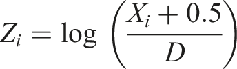

Z_{i} = \log (\frac{X_{i} + 0.5}{D})

Where

X_{i}

, and

Z_{i}

are the untransformed and transformed variables, respectively, for each LoC frequency, and D is the total patient stay on the given day. The imputation was performed with the ward as a cross-sectional variable, the ‘observation time’ as a time stamp, and the day of week as a nominal variable to capture any weekly periodicity. Due to the risk of long tails from the discrete nature of the LoC frequencies, 10 data sets were imputed as opposed to the software default 5 to check for acute shifts in coefficients. Prior to regression analysis the variables were inversely transformed to restore their discrete nature.

Aggregation and analysis

The Ulysses incident data was aggregated by month and ward, and the harm associated with adverse events was dichotomised into “No Harm” events (those labelled as no harm or near miss) and “Harmful” events (all other labels).

Ward-monthly average LoC across all shifts were calculated for each LoC level individually. To make LoC levels more comparable between wards, the previous annual average LoC was subtracted from each monthly average LoC. Subtracting the previous annual average serves the purpose of correcting for between-ward variations in needs due to the typical case load, as well as gradual changes in ward roles. The two data sets were aligned at the month and ward level. This process is outlined in Figure 1.

Figure 1.

Breakdown of data sources through alignment process. ‘Ward-Month’ refers to the aggregated data and indicates 958 unique pairings of ward and month.

The ratio of harmful and non-harmful events in the aggregated data set was analysed via binomial logistic regression in R using the standard generalised linear model functions of the statistics package. The analysis initially considered only a main effects model of three covariates:

• Ward

• Pre or during the Covid-19 initial lockdown (defined as pre or post 1^st March 2020)

• Monthly average patient LoC frequencies (Previous Ward-specific annual average subtracted)

This was subsequently followed by models with interaction terms to investigate if the effect of Ward or variation in LoC changes either side of the initial lockdown measures introduced in England in March 2020. The interaction term models were compared to the main effect models via ANOVA of nested models analysis, using a chi-squared test on deviance residuals. Based on the ANOVA results, an optimal model was selected and summarised via 95% confidence intervals for the relevant coefficients.

Results

DQA step 1

Table 2 presents the DQ summary statistics for the subset of Allocate acuity and Ulysses incident variables used in the binary logistic regression presented later. Of the Allocate acuity variables, five show full completion (‘Ward’, ‘Date’, ‘Census period’, ‘Day of week’ and ‘Status’), with all of the Ulysses incident variables fully completed. Six of the fully completed variables show very high entropy (‘Ward’, ‘Date’, ‘Census Period’ and ‘Day of week’, ‘Department’ and ‘Incident Date’) demonstrating each possible value is well represented in the data. The ‘Status’ variable shows a low entropy, due to the dominance of the ‘Actual’ value, which in this scenario is useful as it demonstrates the majority of LoC observations were made temporally close to the census time. The LoC scores show a mixture of completion percentages, with the Level 0 and Level 1B being most often completed, with the higher LoC scores (Level 2 and 3) often left blank. It is possible that this missingness represents two mechanisms - omission of zeros and missed observations. The ‘Actual Impact’ variable shows a reasonable entropy – dominated by the “1 - No Harm” value (∼68% of entries) but with some evidence of events resulting in a level of harm.

Table 2.

Data quality point estimates for variables drawn into the final analysis (all ‘Status’ included). For statistics for the entire data set see Supplemental Information.

Dataset	Variable	Percent missing	Cardinality	Entropy	Entropy ratio	Modal size (%)	Modal value
Acuity	Ward	0	15	2.70	1	6.9	Charnwood
	Date	0	2637	7.86	1	0.1	21/02/2017
	Census period	0	4	1.27	0.91	43.2	Night
	Level 0	27.2	34	2.72	0.77	27.2	NA
	Level 1A	47.3	35	2.03	0.57	47.3	NA
	Level 1B	21.4	42	3.09	0.83	21.4	NA
	Level 2	74.5	28	1.08	0.33	74.5	NA
	Level 3	92.8	13	0.27	0.1	92.8	NA
Incident	Actual impact	0.00	6	0.87	0.48	68.62	1 - No Harm
	Department	0.00	18	2.65	0.92	13.31	Ward 1
	Incident date	0.00	2000	7.49	0.99	0.16	12/10/2016

During investigating the data, there appear to be two patterns to missing observations; entries where ‘Status’ is either ‘Actual’ or ‘Predicted’ where one or two values were missing, and entries where the ‘Status’ was ‘No Data Entered’ and all five observations were missing. When the data were filtered (excluding ‘Status’ of ‘No Data Entered’) the proportion missing of each patient LoC were correlated with the mean score, with the highest mean score representing the least missing data (highest being Level 1B; mean = 11.9, missing % = 10.7% vs lower being Level 3; mean = 0.06, missing % = 94.9%). It is possible that this missingness represents two mechanisms - omission of zeros and missed observations.

DQA step 2

Initial inspection of the missing information between missingness of LoC scores and other variables in the acuity data set reveals a relationship with the ‘Status’ variable. The ‘Status’ indicates if, and when observations were made relative to the predetermined census period. If the observations are not entered, the variable takes the value ‘No Data Entered’ whereas if the observations are entered, the value is ‘Actual’ if observations are entered within the 2-h window of the census period, and ‘Predicted’ otherwise. The presence of ‘No Data Entered’ shows up with a clear lack of observed LoC scores, with 100% of patient LoC scores missing. Missing LoC scores due to ‘No Data Entered’ made up 37.8% of missing values. Where the status was either ‘Actual’ or ‘Predicted’, it was more common for a single patient LoC frequency to be missing rather than all five, and may not be missing, but shorthand for zero.

With the acuity data filtered by ‘Status’ for ‘Actual’ or ‘Predicted’ observations, the mutual information between the missingness of each patient LoC and the values of the variables were measured and are given in Table 3. It appears that the reporting ‘Ward’, and the frequency of ‘Level 3’ LoC have the greatest influence on when each patient LoC score is missing. Examining the data reveals that missingness of ‘Level 0’, ‘Level 1A’, ‘Level 1B’ and ‘Level 2’ are greatly dependent on the ward, with prevalence of reported zeros correlated to missingness (i.e., wards that reported zeros most often, had the greatest rate of missing data). Hence, it appears likely that these values could be zero and imputing zero values over nulls where some observations were made should be fair and hence was done.

Table 3.

Proportion of entropy of missing data covered by a variable. Columns are the missing variable considered and rows the valued variable.^a

	Level 0	Level 1A	Level 1B	Level 2	Level 3
Ward	0.13	0.24	0.19	0.40	0.15
Date	0.14	0.04	0.09	0.04	0.24
Census period	0.02	0.00	0.00	0.00	0.00
Level 0	1.00	0.22	0.59	0.07	0.00
Level 1A	0.35	1.00	0.56	0.00	0.00
Level 1B	0.44	0.08	1.00	0.00	0.00
Level 2	0.27	0.40	0.93	1.00	0.00
Level 3	0.75	0.80	0.96	0.81	1.00

^aThe table is best read considering each column independently. The first column rates the level of predictive power each variables possessed as to when the ‘Level 0’ variable was not filled in – with “Ward” and “Level 3” showing the highest scores. This indicates a possible relationship between the Ward/‘Level 3’ score and if the ‘Level 0’ variable is recorded.

DQA step 3

A two-stage imputation process has now been followed; imputing zero’s where cases were partially complete (under the assumption these are omitted zero values) and then applying multiple imputation to handle cases of all LoC scores missing. The variable summaries for LoC variables having performed the first zero imputation are given in Table 4.

Table 4.

Data quality point estimates for level of care variables have imputed zero’s on partially complete rows (i.e., omitted values).

Variable	Percent missing	Cardinality	Entropy	Entropy ratio	Modal size (%)	Modal value
Level 0	15.7	34	2.787903	0.79	17	0
Level 1B	15.7	42	3.210763	0.86	15.7	NA
Level 1A	15.7	35	2.204087	0.62	35.9	0
Level [high acuity]	15.7	28	1.327688	0.4	62.7	0

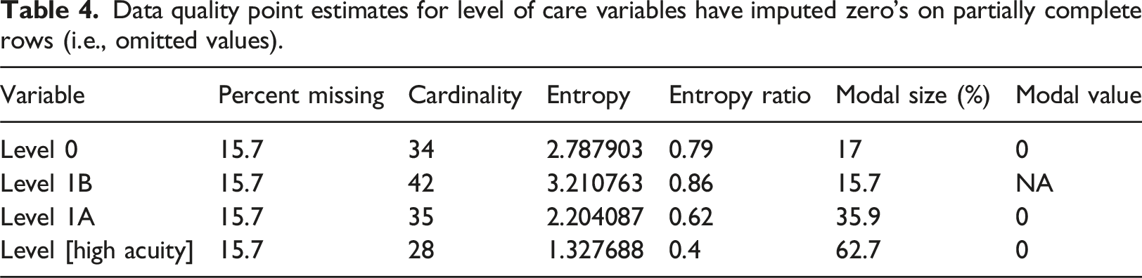
The data set is structured as a time-series-cross-section, with each observed LoC frequency forming a time series within the cross-sectional units of the Ward. A ward (due to specialisation) would be expected to have a greater auto-correlation to previous observations than correlations to other wards in the Trust. Within cross-section auto-correlations of the LoC frequencies were checked via mutual information and, for each LoC, the last observation window shows good evidence of predicting the next value (see SI 4 A for a summary table). Given this behaviour we selected the AMELIA II imputation algorithm as it is explicitly designed for imputation of time-series-cross-sectional data sets. Given the structure of the data we include ‘observation time’, and Ward as key auxiliary variables.

Imputation of each patient LoC frequency (‘Level 0’, ‘Level 1A’, ‘Level 1B’, and ‘High Needs’ [‘Level 2’ + ‘Level 3’]) using the AMELIA II algorithm showed reasonable performance, with Figure 2 shows an example of an over imputed sample from the ‘Level 1A’ scores (similar plots for each LoC frequency can be found in SI2). The over imputed results show good linearity and reasonable breadth of the posterior intervals, suggesting the model will reflect realistic values with reasonable error to capture the possible breadth of values. Hence, the technique appears to have made a good estimate of the data with reasonable accuracy for noise and the pooled results should better reflect uncertainty of the data.

Figure 2.

Subsample of over imputation results for the ‘Level 1A’ patient LoC frequency. Each line represents the oversampled distribution for a complete data point in the study.

Analysis

The ANOVA of nested models indicated that the ‘Prevalence of Harm’ of adverse events did not depend on variations in individual LoC frequencies, but only on the variation in patient numbers (

χ_{3}^{2} = 0.844, p > 0.05

) but the rate before and during the initial Covid-19 lockdown measures was ‘Ward’ specific

(χ_{13}^{2} = 37.31, p < 0.001) .

Hence the reported model features pre- and post-Covid-19 lockdown effects for ward, and the change in patient head count. The 95% CIs are reported for each ward pre-Covid-19 (baseline), the change during the lockdown period, and the effect of change in patient head count in Table 5.

Table 5.

Estimated coefficients of binary logistic regression model for proportion of harm where adverse events have occurred expressed as odds ratios (O.R.).

Type	Term	O.R. estimate	95% CI	Interpretation^a
Baseline^b	Cardiac	0.491	[0.414, 0.582]	N/A
	Discharge/Rehab ward	0.398	[0.262, 0.604]	N/A
	Elective orthopaedic surgical	0.476	[0.382, 0.593]	N/A
	Gastro	0.554	[0.483, 0.636]	N/A
	General medical	0.35	[0.283, 0.433]	N/A
	Geriatric	0.5	[0.434, 0.576]	N/A
	Haematology/Oncology	0.371	[0.317, 0.434]	N/A
	Ortho/Trauma	0.48	[0.42, 0.549]	N/A
	Private ward	0.255	[0.185, 0.353]	N/A
	Respiratory A	0.496	[0.417, 0.59]	N/A
	Respiratory B	0.414	[0.354, 0.485]	N/A
	Short stay medical unit/Covid-19	0.501	[0.43, 0.584]	N/A
	Stroke	0.471	[0.417, 0.533]	N/A
	Surgical A	0.466	[0.387, 0.562]	N/A
	Surgical B	0.55	[0.444, 0.681]	N/A
Level of care (Loc)^c (previous annual average subtracted)	Number of patients (detrended)	1.016	[1.001, 1.03]	*
Covid-19 effect^d (Represents change in O.R. from baseline since 1^st Match 2020)	Cardiac (change during Covid-19)	1.671	[1.295, 2.155]	***
	Discharge/Rehab ward (change during Covid-19)	2.037	[1.291, 3.213]	**
	Elective orthopaedic surgical (change during Covid-19)	1.506	[1.099, 2.063]	*
	Gastro (change during Covid-19)	1.804	[1.489, 2.186]	***
	General medical (change during Covid-19)	2.484	[1.916, 3.221]	***
	Geriatric (change during Covid-19)	1.364	[1.11, 1.675]	**
	Haematology/Oncology (change during Covid-19)	1.557	[1.208, 2.006]	**
	Ortho/Trauma (change during Covid-19)	1.452	[1.188, 1.776]	**
	Private ward (change during Covid-19)	1.872	[1.211, 2.895]	**
	Respiratory A (change during Covid-19)	1.357	[1.057, 1.743]	*
	Respiratory B (change during Covid-19)	1.664	[1.323, 2.092]	***
	Short stay medical unit/Covid-19 (change during Covid-19)	1.025	[0.815, 1.288]	—
	Stroke (change during Covid-19)	1.555	[1.303, 1.855]	***
	Surgical A (change during Covid-19)	1.245	[0.971, 1.596]	—

^aWhere “—” refers to a p-value of (1, 0.05], “*” refers to a p-value of (0.05, 0.005], “**” refers to a p-value of (0.005, 0.001], and “***” refers to a p-value of (0.001, 0]. Interpretations for the baseline coefficients are not performed as they would be comparing to an expected coefficient of zero, i.e., a 50:50 break down of incidents, which has no theoretical underpinning.

^bBaseline O.R. are by ward and represent the shift in odds relative to odds 1.

^cLoC O.R. represent the multiplicative change in odds per unitary change in LoC relative to the previous annual average.

^dCovid-19 Effect O.R. are by ward and represent the change in odds following the introduction of Covid-19 protective measures in March 2020.

In the pre-Covid-19 data it appears that the majority of wards have the same rate of reporting events of harmful: non-harmful events, with the exception of the ‘Private Ward’ which demonstrated a far greater ratio of non-harmful and near miss events. Following the introduction of the initial Covid-19 lockdown response measures, most wards showed a marked increase in the proportion of adverse events reported being harmful, with the ‘Discharge/Rehab Ward’ and ‘General Medical’ wards showing the largest increase in odds ratio.

Considering the role patient acuity plays on reporting culture, the data showed no significant evidence that spiking frequencies of individual LoCs had an effect on the proportion of adverse events reported being harmful. However, increases in patient numbers above average levels do appear to significantly increase the proportion of adverse events reported being harmful.

In this scenario the ANOVA of nested models indicated that the ‘Prevalence of Harm’ of adverse events did not depend on variations in individual LoC frequencies, but only on the variation in patient numbers (

χ_{3}^{2} = 5.21, p > 0.05

) and the rate before and during the initial Covid-19 lockdown measures was not ‘Ward’ specific

(χ_{13}^{2} = 19.47, p > 0.05)

. Hence the reported model features Ward effects, a system wide effect for the initial Covid-19 lockdown, and the change in patient head count. The 95% CIs are reported for each ward (baseline), the change during the lockdown period, and the effect of change in patient head count in Table 6.

Table 6.

Estimated coefficients under listwise deletion of binary logistic regression model for proportion of harm where adverse events have occurred expressed as odds ratios (O.R.).

Type	Term	O.R. estimate	95% CI	Interpretation^¥
Baseline*	Cardiac	0.512	[0.45, 0.583]	N/A
	Charnwood	0.286	[0.229, 0.355]	N/A
	Discharge/Rehab ward	0.516	[0.432, 0.616]	N/A
	Elective orthopedic surgical	0.476	[0.405, 0.559]	N/A
	Gastro	0.611	[0.552, 0.676]	N/A
	General medical	0.572	[0.488, 0.669]	N/A
	Geriatric	0.474	[0.425, 0.527]	N/A
	Hematology/Oncology	0.369	[0.321, 0.424]	N/A
	Ortho/Trauma	0.472	[0.425, 0.524]	N/A
	Respiratory A	0.465	[0.406, 0.531]	N/A
	Respiratory B	0.403	[0.353, 0.458]	N/A
	Short stay medical unit/Covid-19	0.484	[0.421, 0.554]	N/A
	Stroke	0.477	[0.434, 0.523]	N/A
	Surgical A	0.418	[0.367, 0.476]	N/A
	Surgical B	0.367	[0.293, 0.459]	N/A
Level of care (Loc)†	Number of patients (detrended)	1.004	[0.991, 1.018]	—
Covid-19 effect‡	Covid-19 effect	1.515	[1.415, 1.622]	***

^*Baseline O.R. are by ward and represent the shift in odds relative to odds 1.

^†LoC O.R. represent the multiplicative change in odds per unitary change in LoC relative to the previous annual average.

^‡Covid Effect O.R. are by ward and represent the change in odds following the introduction of Covid19 protective measures in March 2020.

^¥Where “-” refers to a p-value of (1, 0.05], “*” refers to a p-value of (0.05, 0.005], “**” refers to a p-value of (0.005, 0.001], and “***” refers to a p-value of (0.001, 0]. Interpretations for the baseline coefficients are not performed as they would be comparing to an expected coefficient of zero, i.e. a 50:50 break down of incidents, which has no theoretical underpinning.

If we compare the models learned from the data with (Table 5) and without (Table 6) imputation and correction for DQ issues we see quite the striking difference. Notably, without the imputation the Covid-19 effects showed no ward dependence; from an operational perspective, if we believe all wards are equally affected, we would distribute our resources evenly, possibly looking for over-arching chronic issues, whereas if we follow the imputed analysis it is far easier to identify ‘Hot Spot’ wards which need individual attention.

Discussion

DQ is a crucial task for leveraging intelligence from routinely collected data, particularly for the NHS in the UK. With a substantial amount of missing data generated, meaningful analyses for adverse event reporting and its consequences are highly challenging for ward-level data. The DQ process illustrated here has focussed on objective measures (Entropy, Cardinality, and Mutual Information) predominantly due to the repeatability and ease of implementation where data already exist. Subjective data quality measures (e.g., timeliness, reliability) are not inherently less valuable – but they do require a greater investment of time and resources where an initial objective analysis can be beneficial in contextualising DQ decisions.³

Our approach of breaking down DQ into three distinct steps (univariate, bivariate and imputation) has aided in structuring the analysis, aiding communication to stakeholders, and improving the transparency of the analysis. While the DQ process identified missing observations as a key concern, the three-step process could be considered as ‘Inspect’, ‘Explore’ and ‘Improve’. Such a paradigm can be tailored to whatever challenges prevail, and the tools/skill sets available. The multiple-step approach is antithetical to a traditional medical statistics approach, as clinical trials demand a highly pre-considered and planned analysis to ensure the minimal risk of multiplicity. For operational decisions/health informatics however, adopting our explorative approach can be beneficial.

The feasibility and necessity of the technique reported here is limited due to the single centre being studied. The results of the analysis may not readily generalise across the health care system, and equivalent data sets may not be readily available to perform an equivalent analysis at a new site. In addition, depending on the scale and mechanism of missingness, it is feasible for a missing-adjusted analysis to result in equivalent results as a non-adjusted analysis, despite having taken time and resource to perform. Such an outcome, however, cannot be determined a priori and the extra expense in time and technical skill accepted.

Conclusions

Handling missing data via techniques such as multiple imputation will remain a controversial issue within clinical trials, predominantly due to the human-dependent decision making around the choice of appropriate strategy (much in the same way prior elicitation limits the use of Bayesian analysis^20–22). However, operational decisions within a clinical setting are inherently different to medical decisions. If a clinical trial is inconclusive, there are existing treatments to rely on. Operationally, decision makers and stakeholders have to make a proactive decision even when studies are inconclusive. The systems are naturally transient, where what was appropriate 30 years ago may no longer be true as systems evolve. Decisions made on moderately reliable evidence are superior to those made on no evidence.

A strong benefit of reliable imputation techniques is the ability to ensure that analysis can be representative of otherwise under-reported (and possibly under-represented) groups. Underserved groups have a greater risk of incomplete data by their very nature, but by leveraging appropriate imputation techniques we can avoid exclusion from analysis. Retaining these individuals in the data will ensure the appropriate decisions are taken to benefit an inclusive population. While the discipline of multiple imputation is gradually expanding the challenge will be to upskill informatics teams²³ and bridge the technical gap between what is possible and what teams can deliver.

Supplemental Material

Supplemental Material - A data quality assurance process to improve the precision of analysis of routinely collected administrative data for the NHS (National Health Service) UK

Supplemental Material for The A data quality assurance process to improve the precision of analysis of routinely collected administrative data for the NHS (National Health Service) UK by Robert M. Cook, Alisen Dube1, Md Asaduzzaman, Tim Beales, Ross Pearce, Luke Blackwell, Claire Whitehouse, Joshua Miller, Malcolm Gough, Mark Radford, Alison Leary and Sarahjane Jones in Health Informatics Journal

Footnotes

Acknowledgments

This study is funded by The Health Foundation under the project NuRS and AmReS: nurse and ambulance workforce retention and safety.

ORCID iDs

Md Asaduzzaman

Joshua Miller

Alison Leary

Sarahjane Jones

Statements and declarations

Author contributions

The study was conceptualized by RC, AD, MD, MG, MR, AL and SJ. Methodology designed by RC, AD, MD, JM, MR, AL and SJ. Formal analysis, R code development and data visualization was carried out by RC. Data curation and resources were carried out by RC, TB, LB, and RP. Project administration was carried out by AD, CW, JM and SJ. Validation was done by MD. The original draft was done by RC, with review and editing by RC, AD, MD, JM, MR, Al, and SJ.

Funding

The authors disclosed receipt of the following financial support for the research, authorship, and/or publication of this article: This work was undertaken as part of the ‘NuRS – Nurse Retention and Safety’ project funded by the Health Foundation as part of their ‘Efficiency Research Programme - Round 3’ (AIMS ID: 1336437).

Conflicting interests

The authors declared no potential conflicts of interest with respect to the research, authorship, and/or publication of this article.

Dedication

This paper is dedicated to our friend and collaborator Malcolm Gough, it was an honour to know you.

Data Availability Statement

Data in anonymised formats may be obtained by request to the corresponding author.

Supplemental Material

Supplemental material for this article is available online.

References

Gandomi

Haider

. Beyond the hype: big data concepts, methods, and analytics. Int J Inf Manag 2015; 35(2): 137–144.

Raghupathi

. Big data analytics in healthcare: promise and potential. Health Inf Sci Syst 2014; 2(1): 3.

Pipino

Lee

Wang

, et al. Data quality assessment. Commun ACM 2002; 45(4): 211–218.

Wang

Strong

. Beyond accuracy: what data quality means to data consumers. J Manag Inf Syst 1996; 12(4): 5–33.

Little

RJA

Rubin

. Statistical analysis with missing data. 3rd ed. Wiley, 2019.

Allison

PD.

Missing data. The SAGE handbook of quantitative methods in psychology. 5th ed. SAGE Publications Ltd, 2009, pp. 72–89.

Donders

ART

van der Heijden

GJMG

Stijnen

, et al. Review: a gentle introduction to imputation of missing values. J Clin Epidemiol 2006; 59(10): 1087–1091.

. Flexible imputation of missing data. 2nd ed. Chapman & Hall/CRC, 2018.

Rubin

. Multiple imputation for nonresponse in surveys. Wiley, 1987.

10.

Buuren

Groothuis-Oudshoorn

. Mice: multivariate imputation by chained equations in R. J Stat Software 2011; 45(3): 1.

11.

Honaker

King

Blackwell

. Amelia II: a program for missing data. J Stat Softw 2011; 45(7): 1.

12.

Stekhoven

Bühlmann

. MissForest—non-parametric missing value imputation for mixed-type data. Bioinformatics 2012; 28(1): 112–118.

13.

Harrell

. Hmisc: harrell miscellaneous. 2023.

14.

Gelman

Hill

, et al. Multiple imputation with diagnostics ( mi ) in R: opening windows into the black box. J Stat Softw. 2011; 45(2): 1–31.

15.

Huque

Carlin

Simpson

, et al. A comparison of multiple imputation methods for missing data in longitudinal studies. BMC Med Res Methodol 2018; 18(1): 168.

16.

Harel

Zhou

. Multiple imputation: review of theory, implementation and software. Stat Med 2007; 26(16): 3057–3077.

17.

Woods

Gerasimova

Van Dusen

, et al. Best practices for addressing missing data through multiple imputation. Infant Child Dev. 2024; 33(1): e2407.

18.

Shannon

. A mathematical theory of communication. Bell System Technical Journal 1948; 27(3): 379–423.

19.

Gray

. Entropy and information theory. 2. Aufl (ed). Springer US, 2011.

20.

Gupta

. Use of Bayesian statistics in drug development: advantages and challenges. Int J Appl Basic Med Res 2012; 2(1): 3–6.

21.

Teira

. Frequentist versus Bayesian clinical trials. Philosophy of medicine. Elsevier B.V, 2011, pp. 255–297.

22.

Yarnell

Abrams

Baldwin

, et al.

Clinical trials in critical care: can a Bayesian approach enhance clinical and scientific decision making?

Lancet Respir Med 2021; 9(2): 207–216.

23.

Robbins

Kyrou

Arvanitis

, et al. Topol digital fellowship aspirants: understanding the motivations, priorities and experiences of the next generation of digital health leaders. Future Healthc J 2022; 9(1): 51–56.

Supplementary Material

Please find the following supplemental material available below.

For Open Access articles published under a Creative Commons License, all supplemental material carries the same license as the article it is associated with.

For non-Open Access articles published, all supplemental material carries a non-exclusive license, and permission requests for re-use of supplemental material or any part of supplemental material shall be sent directly to the copyright owner as specified in the copyright notice associated with the article.

0.00 MB

1.05 MB