Sage Journals: Discover world-class research

Abstract

Discretization is a preprocessing technique used for converting continuous features into categorical. This step is essential for processing algorithms that cannot handle continuous data as input. In addition, in the big data era, it is important for a discretizer to be able to efficiently discretize data. In this paper, a new supervised density-based discretization (DBAD) algorithm is proposed, which satisfies these requirements. For the evaluation of the algorithm, 11 datasets that cover a wide range of datasets in the medical domain were used. The proposed algorithm was tested against three state-of-the art discretizers using three classifiers with different characteristics. A parallel version of the algorithm was evaluated using two synthetic big datasets. In the majority of the performed tests, the algorithm was found performing statistically similar or better than the other three discretization algorithms it was compared to. Additionally, the algorithm was faster than the other discretizers in all of the performed tests. Finally, the parallel version of DBAD shows almost linear speedup for a Message Passing Interface (MPI) implementation (9.64× for 10 nodes), while a hybrid MPI/OpenMP implementation improves execution time by 35.3× for 10 nodes and 6 threads per node.

Keywords

big data classification density-based discretization density estimation supervised discretization

Introduction

Discretization is a preprocessing step in which continuous values of features are transformed into categorical. Specifically, in discretization, a finite number of intervals is provided and values that lie between two consecutive intervals are replaced by a value which characterizes that range. This process can also be considered as a dimensionality reduction methodology since the initial spectrum of a feature’s values is reduced to a smaller finite set of values.^1,2 This paper focuses on supervised discretization, and specifically on its application as a preprocessing step for classification tasks.

The necessity of discretization is due to the fact that a number of existing classifiers and statistical tests, rely on having only discrete data as input. Additionally, with discrete data, the processing time of a classifier can be reduced³ and the results can be easier to interpret, whereas the use of a discretized version of the data can also improve the obtained accuracy by a classifier.^1,4,5 With the big data era, discretization algorithms need to be able to handle such data efficiently without compromising their performance. Hence, it is important to have discretization algorithms that are computationally efficient and can harness the power of high-performance computing, while minimizing the information lost.

Discretization algorithms can be categorized based on some of their main characteristics.¹ A main characteristic is if it is using the class label (supervised) or not (unsupervised), when deciding for the intervals. If a discretizer is independent of a learner then it is static, otherwise it is dynamic. Algorithms that discretize each feature separately are called univariate and if they consider all attributes multivariate. In case only a part of the information of a feature is used when deciding for an interval, the algorithm is considered as local, otherwise as global. Another characteristic is based on whether the intervals are selected simultaneously (direct) or one at a time (incremental). The last two main characteristics of discretizers are the evaluation measure used to select the most appropriate interval and the procedure used to create the intervals (splitting or merging). In the splitting approach, a discretizer starts with an empty set of intervals and each added interval divides the domain, whereas in the merging approach, it begins with a set of intervals which are being merged based on a criterion. In case the algorithm is incremental and uses the splitting approach, it is called Top-Down, whereas if it is using merging, it is called a Bottom-Up approach.

Supervised discretization

In supervised discretization, an algorithm tries to transform each feature from continuous to categorical by using the class label of each instance. By transforming continuous data to discrete, there is the risk of information loss, especially if a very small number of intervals is created. Hence, a discretization algorithm needs to find a balance between the number of intervals created and the information lost.

In Ref.[6], Fayyad and Irani presented an information theory-based discretizer known as MDLP. Its name is from the criterion used for deciding when to stop creating more intervals, the Minimum Description Length Principle, and uses a Top-Down approach. The values of a feature are initially sorted and each midpoint between two consecutive values is considered as a new interval. Then it recursively selects the interval that produces the minimum class information entropy until the stopping criterion is satisfied. A distributed version of MDLP has been proposed⁷ allowing it to be used on big data. Numerous information theory-based algorithms have been proposed in the literature^8–10 but MDLP is one of the most widely used discretizers.

ChiMerge¹¹ is a Bottom-Up discretizer that uses Pearson’s Chi Square test (χ²) to decide if two intervals need to be merged or not. It initially sorts the values of a variable and adds each value in a separate interval. Then it selects the two adjacent intervals with the lowest χ² value and merges them. This is repeated until no adjacent intervals have a χ² value below the predefined threshold. Again, many algorithms were proposed based on χ^212–14 and were found to have good results in Ref [1].

Another Top-Down method is CAIM.¹⁵ This algorithm also sorts the values of a feature and then considers the midpoints between the values as possible intervals. It then repeatedly selects the midpoint that maximizes the class-attribute interdependence as a splitpoint. If the current best value is smaller than the global maximum, the procedure stops. CAIM produces at least C intervals, where C is the number of classes. A version of CAIM that can better handle imbalanced datasets was also proposed,¹⁶ whereas a version for handling multi-label data is also available.¹⁷

Density-based discretization algorithms

The density of a feature can be estimated using parametric or nonparametric methods. Parametric methods are more appropriate when the distribution of the data of a feature follows a known distribution. For example, if the normal distribution is assumed, then a parametric method can be used to calculate the mean and variance of the distribution through maximum likelihood estimates.¹⁸

Nonparametric methods are used when the distribution of a feature is unknown since they can fit different density forms. One such method is kernel density estimation in which a kernel is used with a smoothing parameter for estimating the density of a feature. A simpler method for visualizing such data is the use of histograms, in which the values of a feature are represented by bins and the density of the feature in each bin is shown by its height.

Two well-known discretization algorithms that use binning are the equal-width and equal-frequency discretizers. These are unsupervised methods since they do not take into consideration the class label of the data. Equal-width takes as input the wanted number of bins (k) and creates k equally sized bins. In equal-frequency, k bins with approximately the same number of values are created. These two algorithms did not have a good performance in general in the tests performed in Ref.[1]. A more sophisticated unsupervised density-based discretization (DBAD) algorithm is TUBE,¹⁹ which uses the log-likelihood and cross-validation to select the intervals and decide when to stop splitting the data. It was shown that it can better estimate the density of the data compared to equal-width and equal-frequency in the majority of the tests, where variables had less than 20 unique values, but it is not as fast as equal-width and equal-frequency. A Gaussian mixture model discretization algorithm²⁰ has also been proposed for associative classification of medical data with promising results, but as is the case with TUBE, it is not as fast as the equal-width and equal-frequency approaches.

Contribution

The main contribution of this work is that it turns the fast equal-width unsupervised DBAD algorithm into supervised, while having a performance similar to the state-of-the art supervised discretization algorithms. It initially uses the simple binning approach of the equal-width discretization along with a statistical test to adaptively merge any consecutive bins that have a similar density on each class. Then the resulting intervals of each class are merged to produce a supervised discretization that is computationally efficient. Additionally, the algorithm is parameter-free, thus there is no need to rerun the algorithm multiple times on a dataset to test for different parameter values, which can be a big overhead when dealing with big data.

Methodology

Supervised DBAD

The proposed DBAD algorithm is based on the hypothesis that intervals with different densities can be used to characterize a class and essentially be used to help in separating instances of different classes. For example, Class 1 might have a higher density in the range [0,1], whereas Class 2 in the range of [0.5,2]. Based on this, the following intervals of interest can be created {[0, 0.5], (0.5, 1], (1, 2]} to discretize the data. It is also possible that low-density intervals of a class can help separate it with another class that has no instances in those ranges, hence one should not only focus on identifying the high-density intervals of each class, but instead should identify the intervals in which densities change.

Density-based discretization tries to emulate the way a human would identify similar density intervals with the help of a histogram. Figure 1 illustrates the process followed by DBAD. It begins with equal-width binning (histogram (a)) for estimating the density of a feature in different intervals (bins). Each of the created bins contains a number of instances, which defines the density of the feature in those intervals. The more instances in a bin the higher its density. Once the bins are created, DBAD removes any empty bins by allocating their range to their neighboring non-empty bins (histogram (b)). Then it identifies any consecutive bins with similar densities using a statistical test and merges them (histogram (c)).

Figure 1.

Interval identification for a single class of a feature using density-based discretization (left) and merging of the intervals of each class for identifying the final intervals of a feature (right). The top-left histogram (a) illustrates the initial equal-width binning. Histogram b, illustrates the effect of the removal of the empty bins. The bottom left histogram (c) shows the final bins after merging any consecutive bins with similar densities. The top right (d) histogram shows the intervals selected for Class 1, whereas underneath it (e) the intervals of Class 2 and the bottom-right histogram (f) the final intervals after the ones of the two classes got merged.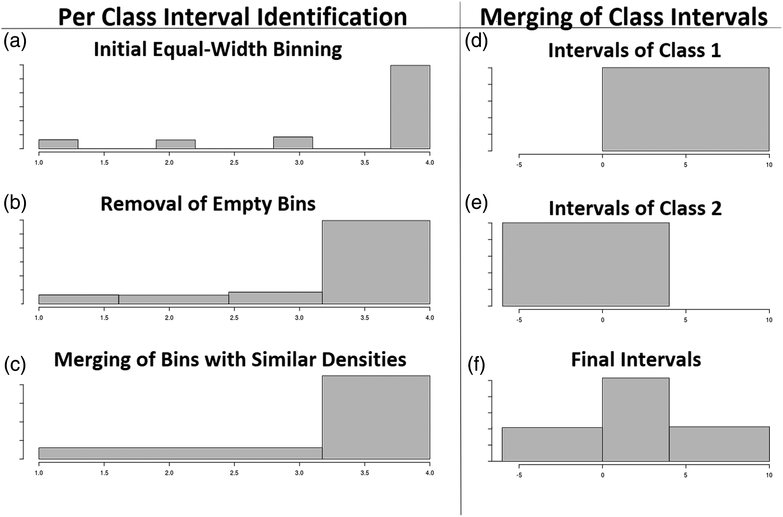

This procedure is performed on the instances of each class of a feature. Once the final intervals of each class are identified, they are merged to obtain the final discretization intervals. An example of the final step of DBAD can be seen on the histograms on the right in Figure 1. As illustrated, Class 1 intervals are in the range [0,10] (histogram (d)), whereas Class 2 intervals are in the range [-6,4] (histogram (e)), so the final intervals for this feature are {[-6, 0], (0, 4], (4,10]} (histogram (f)).

Algorithm 1: DBAD

Require: feature values x

Require: unique class values y

1: featureBins ←∅

2: for each y ∈ y do

3: k ←⌈ log |x^y|⌉ + 1

4: bins ← createEWBins(x^y, k)

5: bins ← removeEmptyBins( bins )

6: bins ← mergeSimilarDensityBins( bins )

7: featureBins ←featureBins⋃ bins

8: end for

9: featureBins ← removeEmptyBins(featureBins)

10: return featureBins

The steps followed by DBAD on a feature are shown in detail in Algorithm 1. The input values of DBAD are the vectors x and y, which contain the values of the feature that will be discretized and the unique class values of the dataset, respectively. To better capture the intervals in which densities change, a proper number of bins (k) needs to be selected. Density-based discretization uses Sturges’ rule²¹ (step 3 in Algorithm 1) for this. Then for each class of the dataset it creates k equal-width bins with the function createEWBins. It then removes any empty bins with the function removeEmptyBins and merges any consecutive bins that have a similar density using mergeSimilarDensityBins. In step 7 of DBAD (Algorithm 1), the intervals of the remaining bins are added in the vector that contains the intervals identified for the other classes for this feature. Once this is done on all of the classes, the function removeEmptyBins is executed (step 9) to remove any empty bins that we might have after the union of the intervals of each class. These are the final intervals that will be used for discretizing the feature.

Algorithm 2 removeEmptyBins

Require: bins

1: i = 1 #indexing starts at 0

2: while i < | bins | do

3: if $b i n s_{i}^{n} = = 0$ then

4: z = i

5: i = i + 1

6: while $b i n s_{i}^{n} = 0$ do

7: $b i n s_{z}^{r i g h t} = b i n s_{i}^{r i g h t}$

8: bins = bins − bins _i

9: i = i + 1

10: end while

11: calculate w using (1)

12: $b i n s_{z - 1}^{r i g h t} = w$

13: $b i n s_{z + 1}^{l e f t} = w$

14: bins = bins − bins _z

15: else

16: i = i + 1

17: end if

18: end while

19: return bins

With equal-width binning it is possible to end up with bins that have no instances in them. To eliminate such bins removeEmptyBins is used (see Algorithm 2). Initially, it merges consecutive empty bins by replacing the right interval of the left empty bin with the right interval of the right empty bin (step 7) and then removing the latter from the bins (step 8). Once the consecutive empty bins are merged, the new empty bin needs to be removed as well. To perform this removal, it is needed to assign its intervals to its surrounding bins. Initially, a new split point (w) is calculated (step 11) using (1)

w \leftarrow b i n s_{z}^{l e f t} + \frac{b i n s_{z - 1}^{n}}{b i n s_{z - 1}^{n} + b i n s_{z + 1}^{n}} * (b i n s_{z}^{r i g h t} - b i n s_{z}^{l e f t})

(1)

where

b i n s_{z - 1}^{n}

and

b i n s_{z + 1}^{n}

represent the number of instances of the bins on the left and right of the empty bin, whereas

b i n s_{z}^{l e f t}

and

b i n s_{z}^{r i g h t}

are the left and right intervals of the empty bin that will be removed. Then the right interval of the bin on the left and the left interval of the bin on the right are replaced by w (steps 12–13) and the empty bin is removed (step 14). This approach ensures that the remaining bins cover the range of the removed bin based on their density, thus bins with more instances (more dense) get a larger range of values. This can be seen in Figure 1. For example, the first two non-empty bins, which have a similar density, shared the empty bin’s space between them, whereas the last bin got the largest share of the empty bin that was on its left because it was much more dense than the third non-empty bin.

Algorithm 3 mergeSimilarDensityBins

Require: bins

1: normalize the bins using (2)

2: i = 1 #indexing starts at 0

3: numBinsM = 1 #num of bins merged with current bin

4: while i < | bins | do

5: $a v g S i z e O f M e r g e d = b i n s_{i - 1}^{n} / n u m B i n s M$

6: $m a x B i n S i z e = \max (a v g S i z e O f M e r g e d, b i n s_{i}^{n})$

7: $m i n B i n S i z e = \min (a v g S i z e O f M e r g e d, b i n s_{i}^{n})$

8: maxMinSize = maxBinSize + minBinSize

9: $p e r c = m i n B i n S i z e / m a x M i n S i z e$

10: CI = confInterval(perc, maxMinSize, 0.05)

11: if 50% ∈ CI then

12: $b i n s_{i - 1}^{r i g h t} = b i n s_{i}^{r i g h t}$

13: $b i n s_{i - 1}^{n} = b i n s_{i - 1}^{n} + b i n s_{i}^{n}$

14: bins = bins − bins _i

15: numBinsM = numBinsM + 1

16: else

17: $b i n s_{i - 1}^{n} = a v g S i z e O f M e r g e d$

18: numBinsM = 1

19: end if

20: i = i + 1

21: end while

22: return bins

The next step of DBAD is to merge any consecutive bins with similar densities (similar number of instances) using mergeSimilarDensityBins. To decide if two consecutive bins have a similar density, a metric is needed which will be less strict with bins representing a small number of instances and stricter with bins of high density. This will enable the identification of intervals in which the densities have a significant difference. This can be tested with a two-tailed test of a population proportion in which the population is the number of instances in the two bins and the hypothesized value of the true population proportion between the two bins is 50%. Essentially the proportion test decides that two bins are similar if 50% is within the calculated confidence interval (CI).

The steps of mergeSimilarDensityBins are shown in Algorithm 3. Initially, two consecutive bins are selected and the bin with the largest and smallest number of instances out of the two is identified (steps 6–7). Then the percentage of the instances of the smallest bin to the sum of the instances of the two is calculated in step 9. Using the calculated percentage and the number of instances of the two bins, the CI at a 5% significance level is calculated (step 10). If 50% is within the calculated CI, the two bins are merged. Initially, the right interval of the bin on the left is set equal to the right interval of the bin on the right (step 12) and the size of the bin on the right is added to the size of the bin on the left (step 13). The bin on the right is then removed from the bins vector (step 14) and the counter of the number of bins contained in the current bin is incremented by one (step 15). Thus, once two or more bins are merged, their new size is the average number of instances of the bins used to create it (avgSizeOfMerged, which is calculated in step 5). The reason for using the average number of instances, is to maintain the density that each bin had separately and have a value that will be comparable with the number of instances of the next bin that will be tested for merging. Once all consecutive similar density bins are merged, the size of the bin that represents them is updated to the value of their average number of instances (step 17).

The range of a CI is affected by the population size since the larger the population the more confident we are on a percentage. In this case, the population size is the number of instances of the two bins DBAD is trying to merge. Specifically, the range of the CI gets narrower as the number of instances increases and hence the criterion becomes stricter. Table 1 represents the number of instances of two bins

(b i n s_{1}^{n}, b i n s_{2}^{n})

, the percentage of bin1

(b i n s_{1}^{n} / (b i n s_{1}^{n} + b i n s_{2}^{n}))

and the calculated CI at a 5% confidence level. As can be seen, for the same percentage, only in the first two cases the 50% criterion is met, but DBAD should merge the two bins in all 4 cases, since 47.6% is very close to 50%.

Table 1.

Confidence intervals as the number of instances increases.

$b i n s_{1}^{n}$	$b i n s_{2}^{n}$	$b i n s_{1}^{n} / (b i n s_{1}^{n} + b i n s_{2}^{n})$	CI
10	11	47.6%	26.4%–69.7%
100	110	47.6%	40.7%–54.6%
1000	1100	47.6%	45.5%–49.8%
10 000	11 000	47.6%	46.9%–48.3%

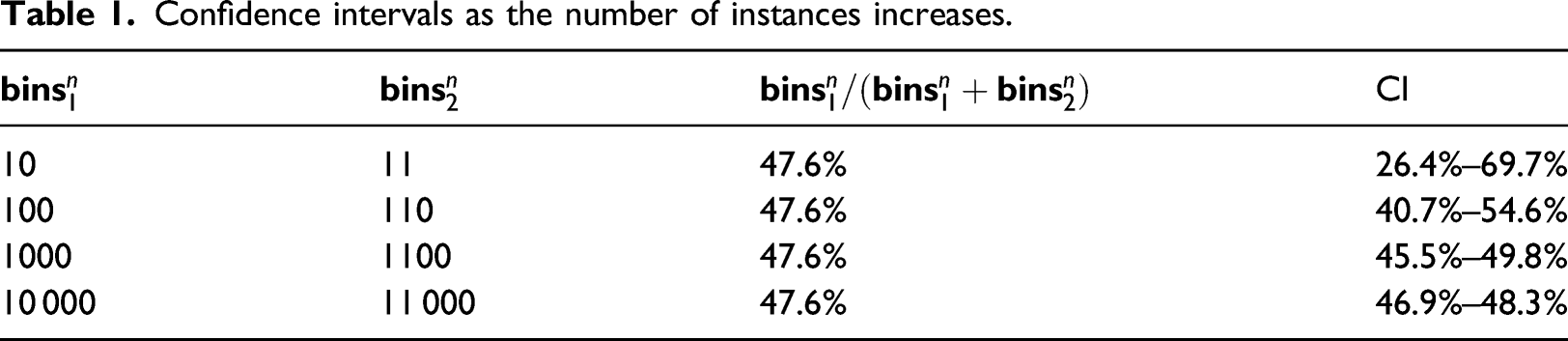
Hence, this approach behaves as needed on low-density bins but can be too strict as the bins’ density increases. To control the strictness of the metric, the sample size of the bins needs to be normalized to have at most α instances in the largest bin using (2)

b i n s_{i}^{n} \leftarrow ⌈ b i n s_{i}^{n} * \frac{\min (α, {b i n s}_{ma x}^{n})}{{b i n s}_{ma x}^{n}} ⌉

(2)

In DBAD, α was empirically set to the value 112, which allows to consider a bin that is consecutive to the largest one as similar if it has at least 75% of its instances.

Parallelization

The algorithm of DBAD can be easily parallelized and executed by multiple resources since each feature can be discretized independently. This is also known as an embarassingly parallel problem that can achieve high-levels of performance. A hybrid parallel version of DBAD that runs on both distributed and shared memory systems using the Message Passing Interface (MPI)²² and OpenMP²³ has been implemented in C++. The algorithm creates multiple MPI processes that will be executed by the available nodes. Each MPI process is scheduled on a separate node in the system, where the DBAD discretization is further parallelized using OpenMP threads (see Figure 2). The algorithm uses as input multiple splitted files of the initial input file to allow processing big data that cannot fit in the RAM of a single node and at the same time reduce the communication overhead between nodes. Initially, MPI is used to distribute the input files evenly to the available nodes. Then each node reads one file at a time and splits its features to the available cores it has and each core executes DBAD on its features. When the cores finish with the discretization of a file, the node returns the discretized version of the file, and the master node merges all results to produce the final output.

Figure 2.

Parallelization of Density-based discretization.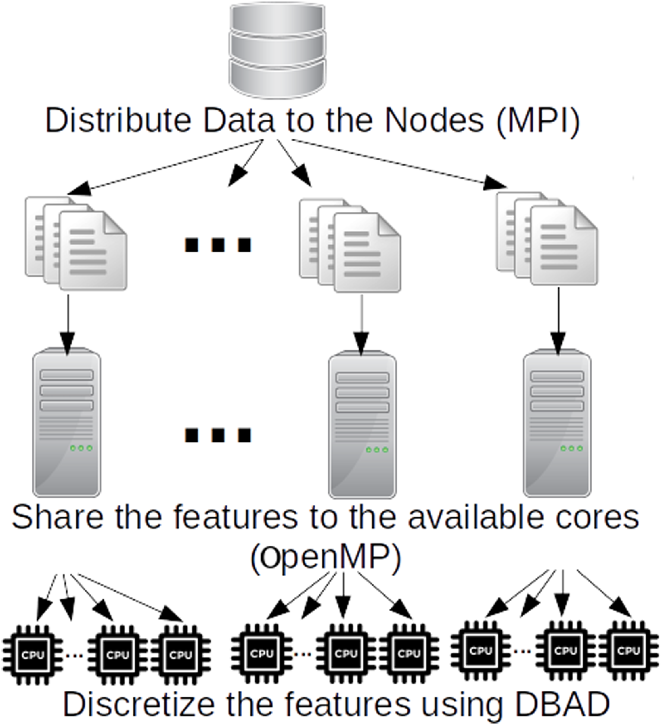

Datasets

A summary of the datasets used in the evaluation is given in Table 2. All of the datasets are from the UCI Machine Learning Repository.²⁴ Since the size of the UCI datasets is of small to medium size, two synthetic big datasets were created to be used for testing the speedup of the parallel version of DBAD.

Table 2.

Summary of the datasets investigated.

Dataset	#Instances	#Features	Instances per class
Heart	270	13 (7)	150/120
SPECTF	267	44 (0)	55/212
Cardiotocography	2126	35 (11)	1655/295/176
Diabetic retinopathy	1151	19 (3)	560/611
Haberman	306	3 (0)	225/81
Saheart	462	9 (1)	302/160
WisconsinBC	569	30 (0)	357/212
Pima	768	8 (0)	500/268
ILPD	583	10 (1)	416/167
Mammographic	830	5 (4)	427/43
Arcene	200	9961 (0)	112/88
Synthetic1	10 000	1000 000 (0)	5000/5000
Synthetic2	1000 000	10 000 (0)	500 000/500 000

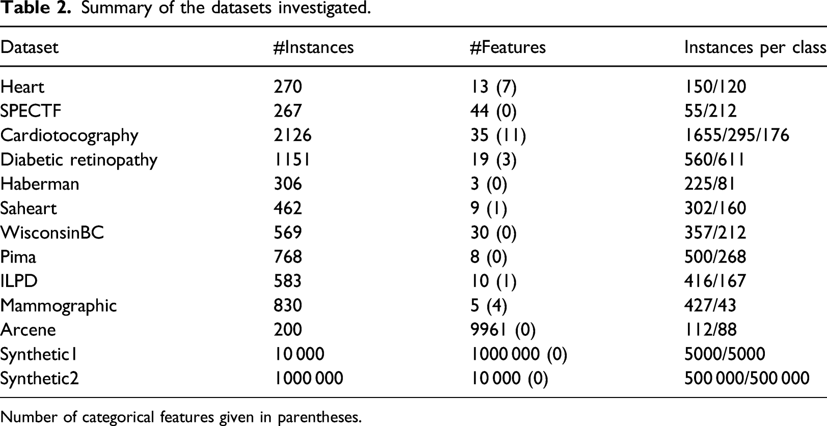
Number of categorical features given in parentheses.

The datasets from the UCI repository cover a wide range of datasets of the life sciences domain. They were selected so as to have different ranges of number of instances and features and have a variety of class balances. These datasets had a two-step preprocessing procedure. The first step was to replace any missing values using (3), which basically replaces the missing values of a variable with its minimum value minus one

x_{\emptyset} \leftarrow \min (x) - 1

(3)

The second was to remove any single-valued features since they did not contain any information that could help with the classification.

The two synthetic datasets were created using different continuous distributions (uniform, Gaussian, and beta) on each feature, to cover some of the common distributions a dataset might have. The Synthetic1 dataset has a large number of features, whereas Synthetic2 dataset has a large number of instances, to test how the algorithm is affected by the size of each dimension.

Evaluation methodology

To evaluate the effectiveness of DBAD at producing meaningful intervals, a 10-fold stratified Cross-Validation (CV) methodology was followed. Initially, the training folds were used by a discretizer so as to create the intervals for each feature. Using these intervals, the training and testing folds were discretized. Then a classifier was trained on the training folds and its accuracy and Cohen’s kappa value was measured on the testing fold. Specifically, the Support Vector Machine (SVM),²⁵ the Random Forest (RF),²⁶ and Naive Bayes (NB) were used for the classification task.

Additionally, the inconsistency rate of the discretizer was calculated on the testing fold. The inconsistency rate is calculated on each feature and it measures the percentage of instances that will be unavoidably misclassified if a single discretized feature is used in a classification. This is due to the fact that after the discretization of a feature, some instances will end up having the same value but their class will differ.

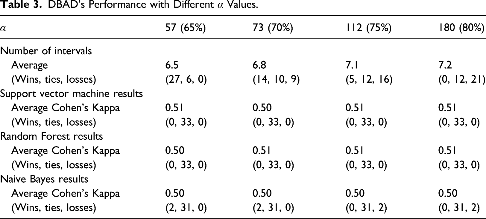
The evaluation was performed among DBAD and three more discretizers which were documented to perform well in the literature.¹ The selected discretization algorithms were CAIM and ChiMerge, which offer excellent performances in different types of classifiers and MDLP which provides a good trade-off between the number of produced intervals and accuracy.¹ To test how the α value of DBAD can affect its results, the values 57 (65%), 73 (70%), 112 (75%), and 180 (80%) were used. All algorithms used the same folds for training and testing during the CV to obtain comparable results.

To test if the intervals created by each discretization algorithm were superior or inferior to DBAD’s intervals, Wilcoxons’ signed-rank test was used on the evaluation measures mentioned above and additionally on the number of intervals produced by each algorithm and its execution time. For the statistical analysis on the sensitivity of DBAD on its α value, initially Friedman’s test was performed and if it was statistically significant, then Wilcoxons’ signed-rank test was used on the different pairs to identify which α value had better results in each scenario. The difference between two algorithms is considered statistically significant if the obtained p-value from the test is less than or equal to 0.05.

The aforementioned evaluation was performed in R. Specifically, from the e1071 package,²⁷ the SVM and NB were used, from the randomForest package,²⁸ RF was used, whereas for the discretization part, the discretization package²⁹ was used for the three discretizers. All of the aforementioned algorithms were used with their default parameters. The version of DBAD used for the aformentioned evaluation was implemented in R to have comparable results with the other discretization methods regarding their execution time.

To test the speedup of the parallel version of DBAD, Synthetic1 and Synthetic2 were split to 10 files each. Specifically, Synthetic1 was split to 10 files with 10,000 instances and 100,000 features each, whereas Synthetic2 was split to 10 files with 1,000,000 instances and 1000 features each. The splitting of the data was necessary for both the parallel and the sequential version of DBAD, so as to be able to load the data in memory, and hence was not considered in the speedup analysis. The speedup was calculated as T₁/T_k, where T₁ is the execution time for discretizing a dataset using a single core and T_k the execution time using k cores. The experiments were run at the Cyprus Institute HPC facility, on nodes with 48 GB of RAM and the Intel Westmere X5650 hexa-core CPUs without hyper-threading. The speedup was tested using a different number of nodes (1–10) and cores (1,2,4,6) per node. This enabled us to identify how the speedup was affected with the increase of the available processing units (cores) in a single node (without the effect of communication delays) and how well it could scale with the addition of more nodes.

Results

In this section, the evaluation results of DBAD are presented. Initially, the analysis on the sensitivity of DBAD’s performance on the α value is shown. Then DBAD’s performance is evaluated against the other discretization algorithms. Initially, results regarding the number of intervals created by each algorithm and the inconsistency rate are presented. Then metrics regarding the performance of the classifiers are shown, which can test the goodness of the intervals and the information lost. The execution time of each algorithm on different datasets is shown and finally the obtained speedup with the parallel version of DBAD is provided. To show if DBAD performed better or worse than another algorithm, the result of the statistical analysis is shown with a sign next to the measure tested. A positive sign indicates that DBAD performed better, whereas a negative sign shows that DBAD had worse performance.

The effect of the α value on DBAD’s performance is shown in Table 3. As expected, with lower α values fewer intervals are created on average, but the difference is less than 1 interval between the smallest and largest α value used. Regarding the Cohen’s Kappa value, the results are similar regardless of the α value. The first two α values had a slightly smaller Cohen’s Kappa value on average on the SVM and RF results, respectively, but the difference was not statistically significant in any of the tested datasets. On the NB results, even though on average all 4 α values had the same Cohen’s Kappa value, the first two (representing 60% and 65%) were found to outperform the other two α values on two datasets, but in general it doesn’t seem that the performance of DBAD can be heavily affected by the α value if it is in the range of values tested.

Table 3.

DBAD’s Performance with Different α Values.

α	57 (65%)	73 (70%)	112 (75%)	180 (80%)
Number of intervals
Average	6.5	6.8	7.1	7.2
(Wins, ties, losses)	(27, 6, 0)	(14, 10, 9)	(5, 12, 16)	(0, 12, 21)
Support vector machine results
Average Cohen’s Kappa	0.51	0.50	0.51	0.51
(Wins, ties, losses)	(0, 33, 0)	(0, 33, 0)	(0, 33, 0)	(0, 33, 0)
Random Forest results
Average Cohen’s Kappa	0.50	0.51	0.51	0.51
(Wins, ties, losses)	(0, 33, 0)	(0, 33, 0)	(0, 33, 0)	(0, 33, 0)
Naive Bayes results
Average Cohen’s Kappa	0.50	0.50	0.50	0.50
(Wins, ties, losses)	(2, 31, 0)	(2, 31, 0)	(0, 31, 2)	(0, 31, 2)

Table 4 provides the average number of intervals created by each algorithm on the training data. In most of the datasets, the smallest number of intervals was created by MDLP and then by CAIM. DBAD is third and created 7 intervals on average on each dataset, whereas ChiMerge had the largest number of intervals in most of the tests.

Table 4.

Average number of intervals.

Dataset	DBAD	MDLP	CAIM	ChiMerge
Heart	5.0	1.7 (−)	2.0 (−)	4.5 (−)
SPECTF	6.7	1.5 (−)	2.0 (−)	4.0 (−)
Cardiotocography	8.7	3.0 (−)	2.7 (−)	14.2 (+)
Diabetic retinopathy	7.5	1.8 (−)	2.0 (−)	46.8 (+)
Haberman	5.0	1.3 (−)	2.0 (−)	3.1 (−)
Saheart	7.4	1.7 (−)	2.0 (−)	17.7 (+)
WisconsinBC	10.1	3.0 (−)	2.0 (−)	44.2 (+)
Pima	9.1	2.1 (−)	2.0 (−)	13.5 (+)
ILPD	7.1	1.6 (−)	2.0 (−)	10.9 (+)
Mammographic	7.2	2.3 (−)	2.0 (−)	3.7 (−)
Arcene	4.0	1.3 (−)	2.0 (−)	7.4 (+)
Average	7.1	1.9	2.1	15.5

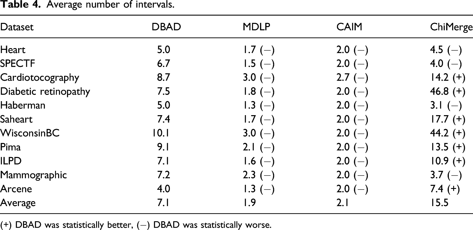
(+) DBAD was statistically better, (−) DBAD was statistically worse.

The inconsistency rate of the testing folds is presented in Table 5. The lowest inconsistency rate was obtained with the original data (NoDiscr), which is essentially the minimum error that can be obtained by a discretization algorithm. The discretization algorithm with the lowest inconsistency rate is ChiMerge and then DBAD follows. MDLP had the worst performance from the discretization algorithms regarding this measure.

Table 5.

Average inconsistency rates.

Dataset	DBAD	NoDiscr	MDLP	CAIM	ChiMerge
Heart	32.3	23.6 (−)	34.5 (+)	33.3 (+)	31.9
SPECTF	19.3	11.5 (−)	20.6 (+)	20.4 (+)	20.0 (+)
Cardiotocography	20.1	17.5 (−)	20.2 (+)	20.2 (+)	19.5 (−)
Diabetic retinopathy	41.2	18.7 (−)	45.0 (+)	43.7 (+)	33.2 (−)
Haberman	25.0	16.0 (−)	25.7	25.5	25.4
Saheart	30.4	10.6 (−)	33.8 (+)	32.3 (+)	27.0 (−)
WisconsinBC	20.4	0.4 (−)	22.9 (+)	22.9 (+)	14.4 (−)
Pima	30.0	16.0 (−)	33.1 (+)	32.4 (+)	29.2
ILPD	27.3	16.7 (−)	28.6 (+)	28.5 (+)	26.7 (−)
Mammographic	27.3	24.8 (−)	28.3 (+)	27.9 (+)	27.6
Arcene	38.7	19.4 (−)	42.2 (+)	39.6 (+)	33.4 (−)
Average	28.4	15.9	30.4	29.7	26.2

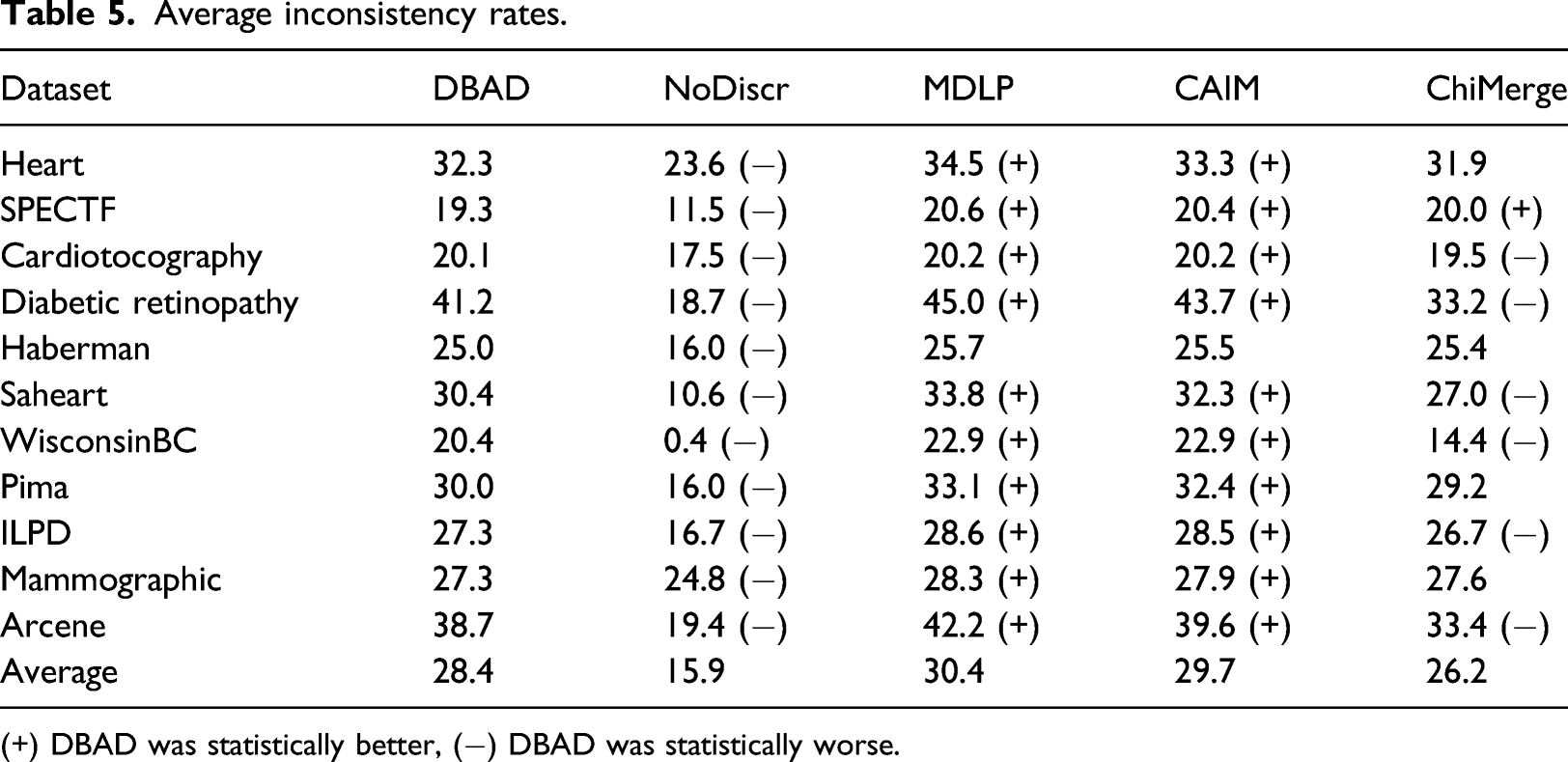
(+) DBAD was statistically better, (−) DBAD was statistically worse.

Table 6 presents the obtained accuracies of the discretized data produced by each algorithm using the three classifiers. The NoDiscr column shows the accuracies obtained with the non-discretized data. As can be seen, DBAD had a similar performance with the other algorithms in the majority of the tests (87%) and performed better (won) 11 times (11%), while it performed worse (lost) in only 2 tests (2%). Additionally, the algorithm had similar or better performance with the non-discretized data and on average had the highest accuracy of all tested discretizers.

Table 6.

Classification accuracy.

Dataset	DBAD	NoDiscr	MDLP	CAIM	ChiMerge
Support vector machine results
Heart	83.7	83.7	84.4	84.1	80.0
SPECTF	78.7	79.0	78.3	79.2	80.6
Cardiotocography	98.8	98.7	99.1	98.8	98.9
Diabetic retinopathy	68.2	69.5	62.3 (+)	63.3 (+)	53.2 (+)
Haberman	72.9	74.8	71.9	74.5	73.2
Saheart	72.1	71.6	70.3	71.2	71.6
WisconsinBC	97.9	97.2	97.0	94.9 (+)	97.2
Pima	75.8	75.5	76.3	73.1	75.4
ILPD	71.3	71.2	70.5	68.2	70.8
Mammographic	82.4	82.9	84.0	83.7	83.1
Arcene	82.4	81.9	66.4 (+)	79.3	70.9 (+)
Random Forest results
Heart	85.6	84.8	85.2	84.8	84.4
SPECTF	81.4	82.5	79.8	81.4	81.8
Cardiotocography	98.9	98.8	99.0	98.8	98.8
Diabetic retinopathy	66.9	68.4	62.6 (+)	63.9 (+)	65.5
Haberman	72.6	74.5	72.6	73.5	74.5
Saheart	72.7	68.4 (+)	70.1	73.0	69.0 (+)
WisconsinBC	96.0	96.5	96.7	95.4	96.8
Pima	77.1	76.8	75.8	75.1	75.4
ILPD	69.3	70.0	69.8	67.9	70.1
Mammographic	81.9	80.6	83.6	84.2 (−)	82.8
Arcene	80.5	82.9	86.0	81.4	82.9
Naive Bayes results
Heart	83.3	78.9	84.4	84.1	81.1
SPECTF	77.6	77.6	77.2	78.3	81.0
Cardiotocography	95.5	95.8	96.6 (−)	96.2	96.4
Diabetic retinopathy	64.4	61.4	62.6	61.8	61.9
Haberman	74.5	71.6	71.9	75.8	73.2
Saheart	68.2	67.5	69.7	72.3	66.3
WisconsinBC	93.8	73.6 (+)	94.2	94.4	93.8
Pima	74.8	66.9 (+)	76.6	72.5	73.7
ILPD	66.9	66.0	67.7	66.4	66.4
Mammographic	83.0	82.8	82.4	81.6 (+)	83.0
Arcene	70.9	67.4	66.4 (+)	66.9	73.0
average	79.5	78.2	78.5	78.8	78.4

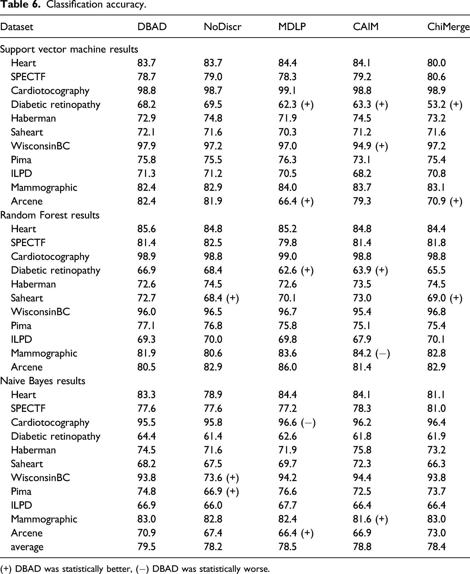
(+) DBAD was statistically better, (−) DBAD was statistically worse.

Table 7 shows the performance of the algorithms on their sensitivity, specificity, and precision. The cardiotocography dataset was not included in this analysis because it has three classes. Regarding the sensitivity measure, DBAD had a similar number of wins and losses against MDLP and ChiMerge but had more wins against CAIM, whereas in specificity it had a similar number of wins and losses against CAIM and ChiMerge but had more wins against MDLP. DBAD performed better more times than the other discretizers in precision. Overall, DBAD performed better than the other algorithms and the non-discretized data in 61 tests and worse in 27 and on average had higher values in all three measures.

Table 7.

Sensitivity, specificity, and precision.

	DBAD	NoDiscr	MDLP	CAIM	ChiMerge
Sensitivity
Average	75.3	71.7	73.9	74.5	73.0	Total
SVM		(2 ,7, 1)	(3 ,6, 1)	(2, 8, 0)	(1, 8, 1)	(8, 29, 3)
RF		(0, 10, 0)	(1, 7, 2)	(0, 9, 1)	(0, 10, 0)	(2, 36, 2)
NB		(5, 4, 1)	(1, 8, 1)	(3, 5, 2)	(2, 7, 1)	(11, 24, 5)
Total		(7, 21, 2)	(5, 21, 4)	(6, 22, 2)	(3, 25, 2)	(21, 89, 10)
Specificity
Average	70.3	68.4	68.7	69.6	69.6	Total
SVM		(1, 6, 3)	(1, 9, 0)	(1, 7, 2)	(1, 7, 2)	(4, 29, 7)
RF		(1, 8, 1)	(4, 5, 1)	(3, 6, 1)	(1, 9, 0)	(9, 28, 3)
NB		(2, 7, 1)	(1, 9, 0)	(1, 8, 1)	(1, 7, 2)	(5, 31, 4)
Total		(4, 21, 5)	(6, 23, 1)	(5, 21, 4)	(3, 23, 4)	(18, 88, 14)
Precision
Average	75.2	70.3	69.3	73.2	72.4	Total
SVM		(1, 8, 1)	(4, 6, 0)	(2, 7, 1)	(2, 7, 1)	(9, 28, 3)
RF		(1, 9, 0)	(4, 6, 0)	(3, 7, 0)	(1, 9, 0)	(9, 31, 0)
NB		(2, 8, 0)	(1, 9, 0)	(1, 9, 0)	(0, 10, 0)	(4, 36, 0)
Total		(4, 25, 1)	(9, 21, 1)	(6, 23, 1)	(3, 26, 1)	(22, 95, 3)

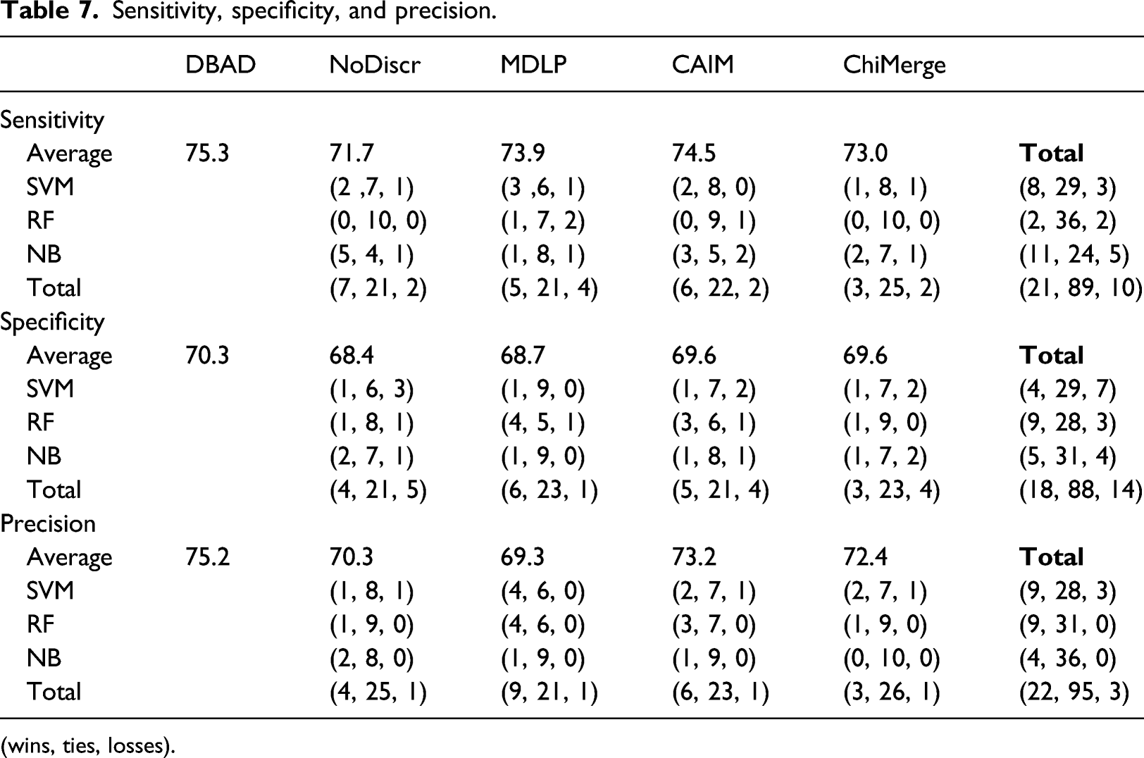
(wins, ties, losses).

The obtained Cohen’s Kappa values are shown in Table 8. As was the case with the accuracy results in Table 6, DBAD had a similar performance with the other algorithms in most of the performed tests. Overall, it performed better than the other algorithms in more tests (15) than it did not (3). Most of its wins were with the SVM classifier as was the case with the accuracy tests.

Table 8.

Cohen’s Kappa values.

Dataset	DBAD	NoDiscr	MDLP	CAIM	ChiMerge
Support vector machine results
Heart	0.67	0.67	0.68	0.67	0.59
SPECTF	0.19	0.01 (+)	0.00 (+)	0.25	0.29 (−)
Cardiotocography	0.97	0.97	0.97	0.97	0.97
Diabetic retinopathy	0.37	0.39	0.26 (+)	0.27 (+)	0.00 (+)
Haberman	0.18	0.18	0.12	0.25	0.20
Saheart	0.33	0.32	0.30	0.34	0.32
WisconsinBC	0.95	0.94	0.94	0.89 (+)	0.94
Pima	0.44	0.44	0.44	0.37	0.43
ILPD	0.09	0.00 (+)	−0.02 (+)	0.09	0.13
Mammographic	0.65	0.66	0.68	0.67	0.66
Arcene	0.65	0.63	0.34 (+)	0.58	0.37 (+)
Random Forest results
Heart	0.71	0.69	0.70	0.69	0.68
SPECTF	0.28	0.29	0.34	0.34	0.32
Cardiotocography	0.97	0.97	0.97	0.97	0.97
Diabetic retinopathy	0.34	0.37	0.27 (+)	0.28 (+)	0.31
Haberman	0.14	0.20	0.16	0.11	0.18
Saheart	0.37	0.25 (+)	0.29	0.37	0.28 (+)
WisconsinBC	0.91	0.92	0.93	0.90	0.93
Pima	0.47	0.48	0.43	0.41 (+)	0.44
ILPD	0.20	0.18	0.02 (+)	0.08	0.22
Mammographic	0.64	0.61	0.67	0.68 (−)	0.66
Arcene	0.66	0.65	0.71	0.61	0.65
Naive Bayes results
Heart	0.66	0.57	0.68	0.68	0.62
SPECTF	0.42	0.24	0.45	0.47	0.44
Cardiotocography	0.88	0.89	0.91 (−)	0.90	0.90
Diabetic retinopathy	0.29	0.24	0.27	0.22 (+)	0.24
Haberman	0.21	0.14	0.12	0.28	0.20
Saheart	0.31	0.26	0.34	0.38	0.26
WisconsinBC	0.87	0.41 (+)	0.88	0.88	0.87
Pima	0.45	0.27 (+)	0.48	0.37 (+)	0.42
ILPD	0.31	0.23	0.31	0.27	0.25
Mammographic	0.66	0.66	0.65	0.63	0.66
Arcene	0.42	0.36	0.34	0.35	0.45
average	0.51	0.46	0.47	0.49	0.48

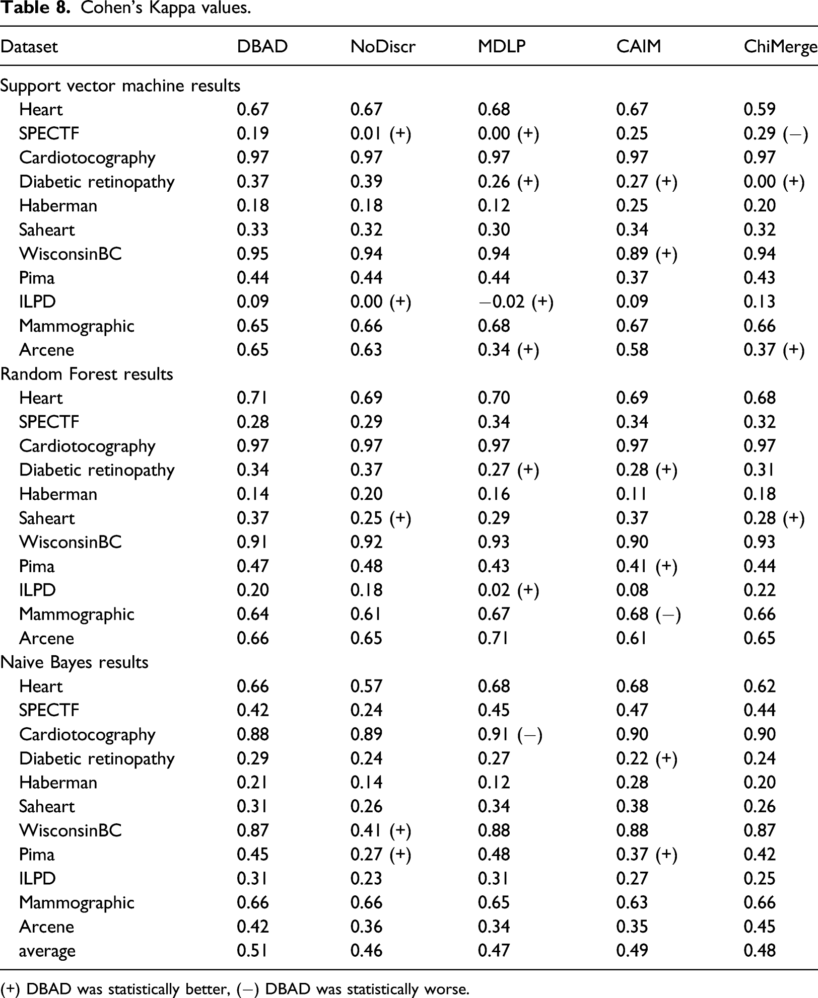
(+) DBAD was statistically better, (−) DBAD was statistically worse.

The average execution time of each discretization algorithm on the training folds is provided in Table 9. Density-based discretization has the lowest computational complexity from the rest of the algorithms, which explains the results shown in Table 9. Density-based discretization is the fastest and in some tests it is at least an order of magnitude faster than the rest. The difference is more obvious in the Arcene dataset, which has the largest number of features from all the datasets. In this dataset, DBAD is approximately 4 times faster than MDLP, 9 times faster than CAIM, and 32 times faster than ChiMerge.

Table 9.

Average execution time in seconds.

Dataset	DBAD	MDLP	CAIM	ChiMerge
Heart	0.03	0.15 (+)	0.42 (+)	1.45 (+)
SPECTF	0.25	0.70 (+)	2.14 (+)	3.78 (+)
Cardiotocography	0.23	2.68 (+)	18.69 (+)	100.13 (+)
Diabetic retinopathy	0.14	3.62 (+)	28.78 (+)	453.44 (+)
Haberman	0.02	0.04 (+)	0.15 (+)	0.22 (+)
Saheart	0.06	0.81 (+)	3.33 (+)	29.27 (+)
WisconsinBC	0.21	10.17 (+)	31.14 (+)	408.20 (+)
Pima	0.05	0.75 (+)	3.11 (+)	21.83 (+)
ILPD	0.05	0.56 (+)	2.20 (+)	8.91 (+)
Mammographic	0.01	0.10 (+)	0.24 (+)	0.34 (+)
Arcene	68.77	300.58 (+)	632.32 (+)	2199.30 (+)
Average	6.3	29.1	65.7	293.4

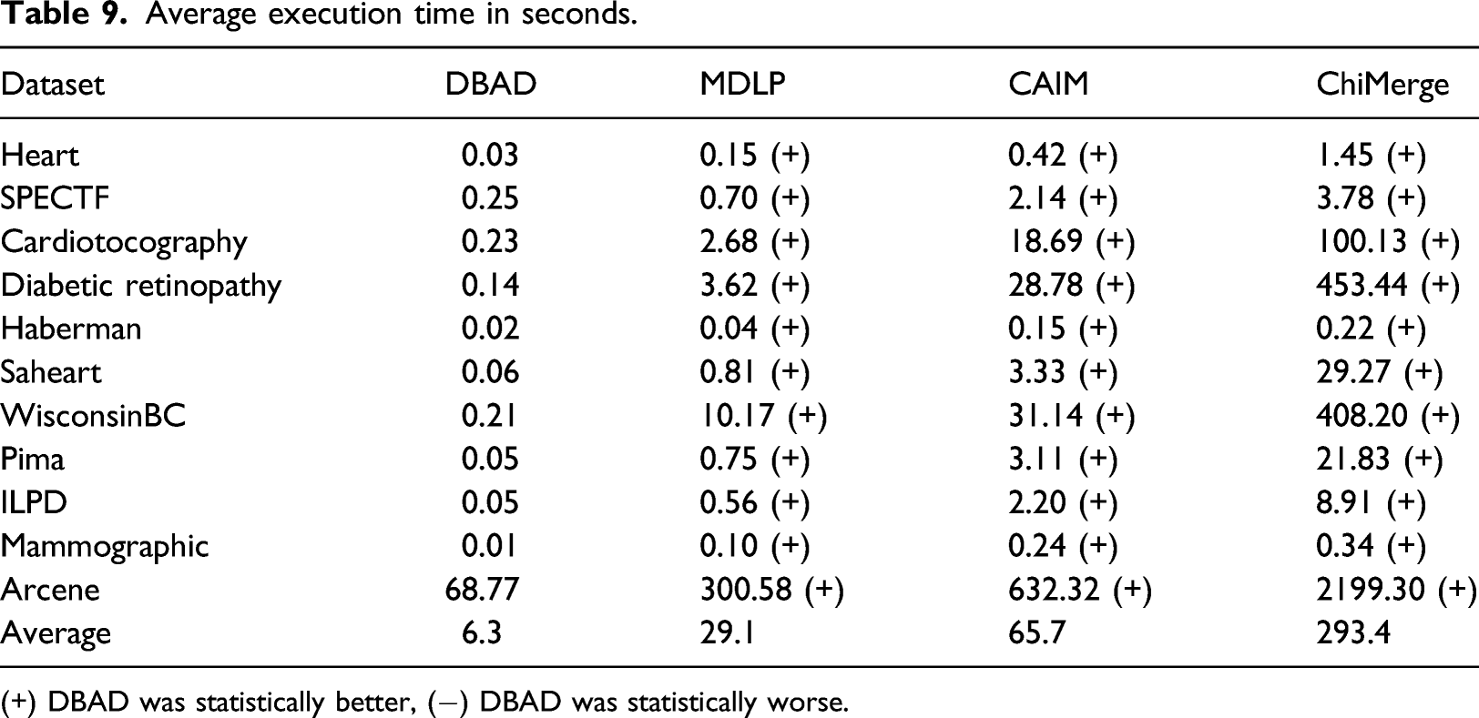
(+) DBAD was statistically better, (−) DBAD was statistically worse.

Table 10 provides the obtained speedup of the parallel version of DBAD. Each cell in the table represents a scenario that the parallel DBAD was tested. In each scenario, a different number of nodes (columns) and a different number of cores per node (rows) were available. For example, in the top-left cell, the speedup of using a single node and a single core is shown, whereas the bottom-right cell shows the obtained speedup when using 10 nodes with 6 cores per node (a total of 60 cores). The time needed to discretize the Synthetic1 dataset with a single node and a single thread was 233 min (approximately 3.9 h), whereas Synthetic2 needed 217 min (7% faster). The first thing worth mentioning is that the speedup was similar in both synthetic datasets, which indicates that the parallel execution is not affected when the number of instances or number of features is much larger than the other. The second thing we notice is that when the number of nodes was set constant and only the number of available cores per node increased (see each column separately), which is also illustrated in Figure 3, even though the speedup increased it did not scale linearly, in fact, it was closer to a logarithmic scaling and hence after some point the addition of more cores per node would not provide any additional gain in speedup. Regarding the scenarios in which the number of cores available per node was stable but the number of nodes increased, we considered T₁ as the time a single node with the number of its available cores needed to discretize a dataset and T_k the time needed when using k nodes and hence k times more cores, similar to the approach followed in Ref.[30] The results are illustrated in Figure 4, where we notice that there is a linear speedup when the number of splits (10) is divisible by the number of nodes.

Table 10.

Speedup of the parallel implementation over the sequential execution time.

#Cores per node	#Nodes
#Cores per node	Dataset	1	2	3	4	5	10
1	Synthetic1	1.0	2.0	2.5	3.3	4.9	9.9
1	Synthetic2	1.0	2.0	2.5	3.3	4.9	9.6
2	Synthetic1	1.7	3.5	4.3	5.7	8.6	17.2
2	Synthetic2	1.8	3.4	4.3	5.7	8.6	17.1
4	Synthetic1	2.7	5.4	6.6	9.1	13.5	26.3
4	Synthetic2	2.8	5.6	7.0	9.4	14.1	28.0
6	Synthetic1	3.3	6.7	8.4	11.1	16.4	33.3
6	Synthetic2	3.8	7.0	8.9	11.8	17.8	35.3

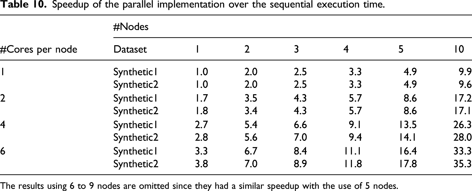
The results using 6 to 9 nodes are omitted since they had a similar speedup with the use of 5 nodes.

Figure 3.

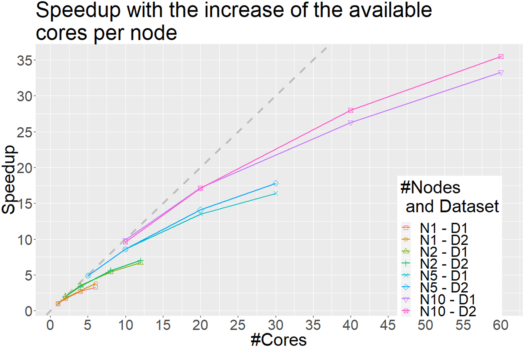
The x axis represents the number of cores and the y axis the obtained speedup compared to using a single node with a single core. Each line represents a different scenario. For example, N1–D1 represents the scenario in which a single node is used to discretize the Synthetic1 dataset (D1) with an increase in the number of available cores, whereas N10–D2 the scenario in which 10 nodes are used for the discretization of the Synthetic2 dataset with an increase in the number of available cores per node. Each point on the lines represents the total number of cores available when the speedup is calculated. The dashed gray line represents the optimal linear speedup. Only scenarios where the number of splits is divisible with the number of nodes are illustrated.

Figure 4.

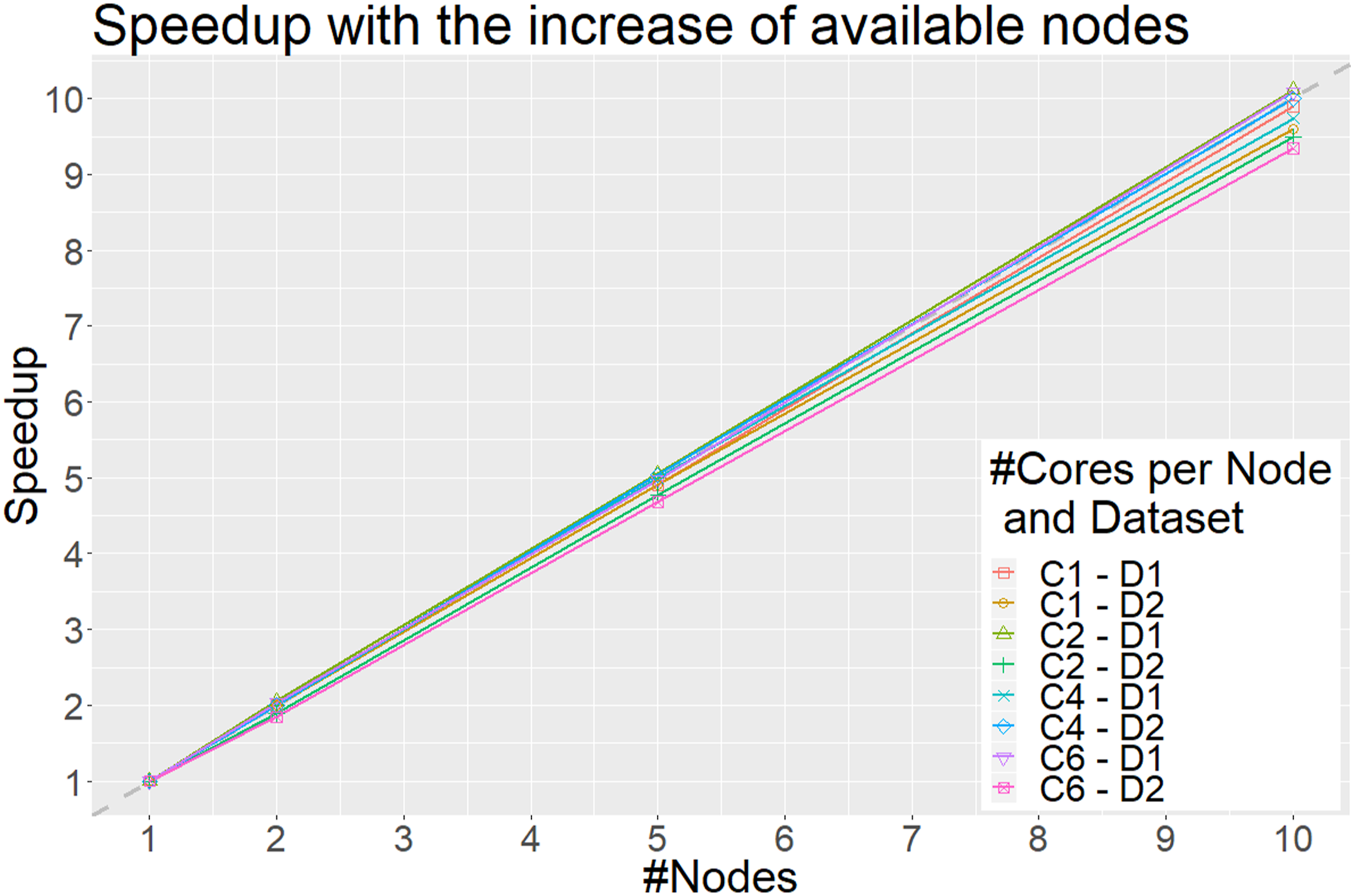
The x axis represents the total number of nodes and the y axis the obtained speedup when increasing the number of nodes (and hence also the number of total cores) compared to using a single node with a specified number of available cores. Each line represents a different scenario. For example, C1–D1 represents the scenario in which each node uses only a single core to discretize the Synthetic1 dataset (D1), whereas C6–D2 the scenario in which each node uses 6 cores to discretize the Synthetic2 dataset. Each point on the lines represents the total nodes used. The dashed gray line represents the optimal linear speedup. Only scenarios where the number of splits is divisible with the number of nodes are illustrated.

Discussion

An important feature of a discretization algorithm is to be able to produce a small number of intervals. Even though MDLP and CAIM performed better on this task, DBAD produced a reasonable number of intervals, whereas ChiMerge produced the largest number of intervals. DBAD might produce a large number of intervals in the case of datasets with many classes with different distributions. This is due to the fact that the intervals are created per class and if the densities are in different intervals on each class, we will end up with much more intervals. On the other hand, this might not negatively affect a classifier’s performance since it could further help with the separation of the classes.

The results regarding the inconsistency rates seem to be associated with the number of intervals produced by the algorithms. As was also found by Ref.[1] the more intervals an algorithm creates, the lower its inconsistency rate is. The performance on this metric does not seem to be correlated with the performance of the classifiers. If that was the case, then the non-discretized data would have produced better results than the discretized.

The results on the obtained accuracies, indicate that DBAD had a similar or better performance compared to the other algorithms in the majority of the tests and in only 2% of the performed tests its performance was worse. Additionally, when using the SVM classifier, it did not perform worse than any of the other methods. A positive outcome of this analysis is that DBAD’s discretization did not significantly reduce the information of the datasets since it performed equally or better than the original datasets in all of the tests. In general, discretization can help increase the accuracy of a classifier, since it can reduce noise from the data and hence reduce overfitting,¹ but in case there is high information loss from the process the opposite results will occur.⁵ The results on specificity indicate that it had a similar performance with the other methods on this measure, while it was able to perform better than the other algorithms more times than they did when considering sensitivity and precision. Cohen’s kappa values also had more tests in which DBAD had a better performance than the other discretization algorithms (15 wins and 3 losses). Since this measure takes into consideration random hits³¹ and many of the tested datasets were imbalanced, it is more appropriate as a measure to compare the efficiency of the discretization algorithms. On average, DBAD had the highest scores in all of the aforementioned measures and since the statistical analysis indicates that it performs similarly or better than the other algorithms in the majority of the tests, there is a good indication that using the regions in which density changes per class is a promising approach for data discretization.

For the aforementioned results, the datasets used in the experiments were of a small to medium size and did not include many non-binary classification tasks, hence some hypotheses could not be fully examined. Since only one dataset had more than two classes (Cardiotocography), it is not clear how well the algorithm can perform with such a dataset. In the Cardiotocography dataset, DBAD produced a larger number of intervals compared to its average, but this was also the case for the rest of the discretizers (except ChiMerge). The performance of the classifiers using DBAD’s discretized version of Cardiotocography was not negatively affected, except in the case of NB which had better results using MDLP’s version. Since there aren’t more tests on such cases, no clear conclusion can be made regarding the effect of the number of classes to the number of produced intervals and its effect on the classifiers’ performance. Finally, since there aren’t any real-world big datasets in the experiment, it is not possible to conclude if the algorithm would have created better intervals and help the classifiers’ performance since with more data it is expected that the true density of the variables would be revealed. Similarly, the other discretization algorithms could have also benefited from larger datasets and produce better intervals as well.

The proposed algorithm has a clear advantage over the others regarding its computational complexity. A dataset can be discretized by DBAD in O(m*n), where m is the number of features and n is the number of instances. Specifically, for a single feature, the binning and number of instances in each bin can be calculated with a single pass from the feature’s data (O(n)), whereas the removal of empty bins and the merging of similar density bins is O(log(n)) since this is approximately the number of bins that are initially created using Sturges’ rule. Algorithms like CAIM, MDLP, and ChiMerge, have a computational complexity of at least O(n* log(n)) for each feature, since this is the complexity for sorting the data. Then the Top-Down approaches have an additional cost of O(k*n), where k is the number of intervals created. For CAIM and MDLP, this value is close to the number of classes and since this is much smaller than the number of instances their complexity is O(m*n* log(n)). Due to the fact that ChiMerge merges two consecutive points/bins at a time, this means that it has an additional complexity of O((n − k)*n), and hence its complexity for discretizing a dataset is O(m*n²). Based on this analysis, it is clear that DBAD has a low computational complexity, which explains its small execution times on the performed experiments.

In addition to its low complexity, DBAD is an embarrassingly parallel algorithm, since each feature can be discretized separately, which enables the use of the algorithm on big data. This also means that the parallelization is limited by the number of features since we cannot use more cores than the available number of features in a dataset. When increasing the number of available cores in a node, the obtained speedup is not linear, similar to the results of the parallel version of MDLP⁷ on a larger dataset, because the overhead of reading the dataset in memory and writing the discretized version of the dataset dominates the total execution time for discretizing the data. The reading and writing tasks are sequential and cannot be parallelized and once the parallel task of the discretization becomes faster than the time needed to read and write the data, no additional speedup can be obtained. Similarly to the results of the parallel MDLP, we expect that the obtained speedup will be lower in smaller datasets since the overhead of data distribution will be larger than the computational part of the discretization and hence the parallel version of DBAD should be applied on big data. On the other hand, when testing the scalability of the algorithm (Figure 4), as performed in Ref.[30] by adding more nodes that have the same number of available cores each, the algorithm shows that it can scale linearly. In Ref.[30], they were able to utilize 82% of the available processing power using four nodes with 8 computing cores each when they scaled from a single node of 8 computing cores, whereas in DBAD more than 90% is utilized using 10 nodes with 6 computing cores when we scaled from a single node of 6 computing cores, which shows that the algorithm has good scalability. Since the reading and writing of each file can be done in parallel in each node, it provides a linear speedup compared to only using a single node with the same number of available cores per node. To get the optimal speedup of DBAD in a distributed system, one should split the initial data to a number of files that is divisible with the number of nodes that will be used. This will allow an optimal load balancing to each node. It is also worth mentioning that the initial splitting of the dataset into smaller subsets will have an overhead which will depend on the speed of the storage disk of the system.

In general, DBAD is a good choice for the fast discretization of data for classification tasks. A limitation of the algorithm is that it will under-perform if for a feature, the data of each class to be discretized are from the same uniform distribution. In such cases, since the density is the same in the entire range of values for all classes, DBAD will not be able to identify any intervals and will return a single-valued feature. In case this feature is interacting with another one, then this information will be lost. On the other hand, DBAD has an advantage over methods that use measures based on class separability, in cases that the data of each class of features are from different distributions and have interactions with low main effects. In such cases, a single feature does not have enough information for separating the different classes unless it is considered in combination with other features, and hence a univariate method that uses a measure based on class separability will return a single-valued feature. DBAD would still be able to split such features based on their density differences and those splits could allow the identification of interacting features. Another limitation of the algorithm is that the initial number of bins selected per class using Sturges’ rule, is the same for all features and it is known that this rule works better on Gaussian data.³² This limitation is handled up to a point by the adaptive merging of the initially created bins that have a similar density by DBAD, but there will be cases that this will not be enough if the initial number of bins is smaller than what is needed. A solution to this would be to use an adaptive algorithm for selecting the initial number of bins per feature,^19,33,34 but usually such methods have extra parameters that need to be fine-tuned or are computationally expensive, which is not desirable when coping with big data.

Conclusions

A new supervised discretization algorithm has been proposed based on how the density of the values of a feature changes for each class. DBAD is a univariate discretizer and hence does not consider any possible feature interactions when selecting the best intervals for each feature, but results indicate that it does not significantly reduce the information contained in a dataset. It is a static discretizer since it is independent of the classifier that will be used at the processing step, which allows it to produce more generic intervals that can perform well with different classifiers. It initially creates all of the bins simultaneously and then follows a bottom-up approach for merging consecutive bins with similar densities, based on the CI of their percentage.

In the performed evaluation, DBAD produced an acceptable number of intervals and had comparable results with the other discretizers. An advantage it has over the other methods is its low computational complexity and the fact that it has no parameters that need to be optimized, hence discretization will be faster than the other tested supervised discretizers on big data. Another reason DBAD can be easily applied to big data is that it is an embarrassingly parallel algorithm since each feature can be discretized independently. Our experiments have shown that even though it doesn’t have a linear speedup with the addition of processing cores it can benefit from them and it scales linearly with the addition of more nodes.

The results of the evaluation indicate that DBAD is a promising approach and needs to be further investigated. One possible direction is to test different methods for the initial binning of the data since the current approach is based only on the number of instances and hence the true distribution of the data might be misrepresented. Another possible direction could be on having an additional step for further reducing the number of the final intervals of each feature based on other metrics.

Footnotes

Declaration of conflicting interests

The author(s) declared no potential conflicts of interest with respect to the research, authorship, and/or publication of this article.

Funding

The author(s) disclosed receipt of the following financial support for the research, authorship, and/or publication of this article: This work was co-funded by the European Regional Development Fund and the Republic of Cyprus through the Research Promotion Foundation (Project Cy-Tera ΝΕΑ ϒΠΟΔΟΜΗ/ΣΤΡΑΤΗ/0308/31).

ORCID iD

Aristos Aristodimou

References

Garcia

Luengo

Sáez

, et al. A survey of discretization techniques: Taxonomy and empirical analysis in supervised learning. IEEE Trans Knowledge Data Eng 2013; 25(4): 734–750.

Ali

Siddiqi

Lee

. Rough set-based approaches for discretization: a compact review. Artif Intelligence Rev 2015; 44(2): 235–263.

Richeldi

Rossotto

. Class-driven statistical discretization of continuous attributes. In: European conference on machine learning, Berlin, Heidelberg, 25–27 April 1995. Springer, pp. 335–338.

Dougherty

Kohavi

Sahami

. Supervised and unsupervised discretization of continuous features. In: Machine learning proceedings 1995, California, 9–12 July 1995. Elsevier; 1995, pp. 194–202.

Kotsiantis

Kanellopoulos

. Discretization techniques: a recent survey. GESTS Int Trans Computer Sci Eng 2006; 32(1): 47–58.

Fayyad

Irani

. Multi-interval discretization of continuous-valued attributes for classification learning. In: IJCAI, pp. 1022–1029.

Ramírez-Gallego

García

Mouriño-Talín

, et al. Data discretization: taxonomy and big data challenge. Wiley Interdisc Rew: Data Mining Knowledge Discov 2016; 6: 5–21.

Zighed

Rabaséda

Rakotomalala

. FUSINTER: a method for discretization of continuous attributes. Int J Uncertainty, Fuzziness Knowledge-Based Syst 1998; 06(03): 307–326.

Liu

Wang

. A discretization algorithm based on a heterogeneity criterion. IEEE Trans Knowledge Data Eng 2005; 17(9): 1166–1173.

10.

Wen

Min

Wang

. A two-stage discretization algorithm based on information entropy. Appl Intelligence 2017: 1–17.

11.

Kerber

. Chimerge: discretization of numeric attributes. In: Proceedings of the tenth national conference on Artificial intelligence, San Jose, California, July 12–16 1992. Aaai Press, pp. 123–128.

12.

Liu

Setiono

. Feature selection via discretization. IEEE Trans Knowledge Data Eng 1997; 9(4): 642–645.

13.

Tay

FEH

Shen

. A modified chi2 algorithm for discretization. IEEE Trans Knowledge Data Eng 2002; 14(3): 666–670.

14.

Gonzalez-Abril

Cuberos

Velasco

, et al. Ameva: an autonomous discretization algorithm. Expert Syst Appl 2009; 36(3): 5327–5332.

15.

Kurgan

Cios

. CAIM discretization algorithm. IEEE Transactions Knowledge Data Eng 2004; 16(2): 145–153.

16.

Cano

Nguyen

Ventura

, et al. ur-CAIM: improved CAIM discretization for unbalanced and balanced data. Soft Comput 2016; 20(1): 173–188.

17.

Cano

Luna

Gibaja

, et al. Laim discretization for multi-label data. Inf Sci 2016; 330: 370–384.

18.

Scott

. Multivariate density estimation and visualization. In: Handbook of computational statistics. Berlin, Heidelberg: Springer, 2012, pp. 549–569.

19.

Schmidberger

Frank

. Unsupervised discretization using tree-based density estimation. PKDD, volume 5. Berlin, Heidelberg: Springer, pp. 240–251.

20.

Khanmohammadi

Chou

C-A

. A gaussian mixture model based discretization algorithm for associative classification of medical data. Expert Syst Appl 2016; 58: 119–129.

21.

Sturges

. The choice of a class interval. J Am Stat Assoc 1926; 21(153): 65–66.

22.

Walker

Dongarra

. Mpi: a standard message passing interface. Supercomputer 1996; 12: 56–68.

23.

Dagum

Menon

. Openmp: an industry-standard api for shared-memory programming. Comput Sci Eng 1998; 5: 46–55.

24.

Lichman

. UCI machine learning repository, 2013. http://archive.ics.uci.edu/ml.

25.

Cortes

Vapnik

. Support-vector networks. Machine Learn 1995; 20(3): 273–297.

26.

Breiman

. Random forests. Machine Learn 2001; 45(1): 5–32.

27.

Meyer

Dimitriadou

Hornik

, et al. Misc functions of the department of statistics, probability theory group (Formerly: E1071). TU Wien, 2017. URL, https://CRAN.R-project.org/package=e1071. R package version 1.6-8.

28.

Liaw

Wiener

. Classification and regression by randomforest. R News 2002; 2(3): 18–22. http://CRAN.R-project.org/doc/Rnews/.

29.

Kim

. Discretization: data preprocessing, discretization for classification, 2012. https://CRAN.R-project.org/package=discretization. R package version 1.0-1.

30.

Segatori

Bechini

Ducange

, et al. A distributed fuzzy associative classifier for big data. IEEE Trans Cybernetics 2018; 48(9): 2656–2669.

31.

Cohen

. A coefficient of agreement for nominal scales. Educ Psychol Measurement 1960; 20(1): 37–46.

32.

Scott

. Sturges’ rule. Wiley Interdiscip Rev Comput Stat 2009; 1(3): 303–306.

33.

Anderson

Mahle

Doom

, et al. Dynamic adaptive binning: an improved quantification technique for nmr spectroscopic data. Metabolomics 2011; 7(2): 179–190.

34.

Wang

Dengdenpehc

. Density peak based efficient hierarchical clustering. Inform Sci 2016; 373: 200–218.

A fast supervised density-based discretization algorithm for classification tasks in the medical domain

Abstract

Keywords

Introduction

Supervised discretization

Density-based discretization algorithms

Contribution

Methodology

Supervised DBAD

Parallelization

Datasets

Evaluation methodology

Results

Discussion

Conclusions

Footnotes

Declaration of conflicting interests

Funding

ORCID iD

References