Sage Journals: Discover world-class research

Abstract

Guillain-Barré Syndrome (GBS) is a neurological disorder affecting people of any age and sex, mainly damaging the peripheral nervous system. GBS is divided into several subtypes, in which only four are the most common, demanding different treatments. Identifying the subtype is an expensive and time-consuming task. Early GBS detection is crucial to save the patient’s life and not aggravate the disease. This work aims to provide a primary screening tool for GBS subtypes fast and efficiently without complementary invasive methods, based only on clinical variables prospected in consultation, taken from clinical history, and based on risk factors. We conducted experiments with four classifiers with different approaches, five different filters for feature selection, six wrappers, and One versus All (OvA) classification. For the experiments, we used a data set that includes 129 records of Mexican patients and 26 clinical representative variables. Random Forest filter obtained the best results in each classifier for the diagnosis of the four subtypes, in the same way, this filter with the SVM classifier achieved the best result (0.6840). OvA with SVM classifier reached a balanced accuracy of 0.8884 for the Miller-Fisher (MF) subtype.

Keywords

feature selection methods multiclass classification single classifiers performance measures predictive model

Introduction

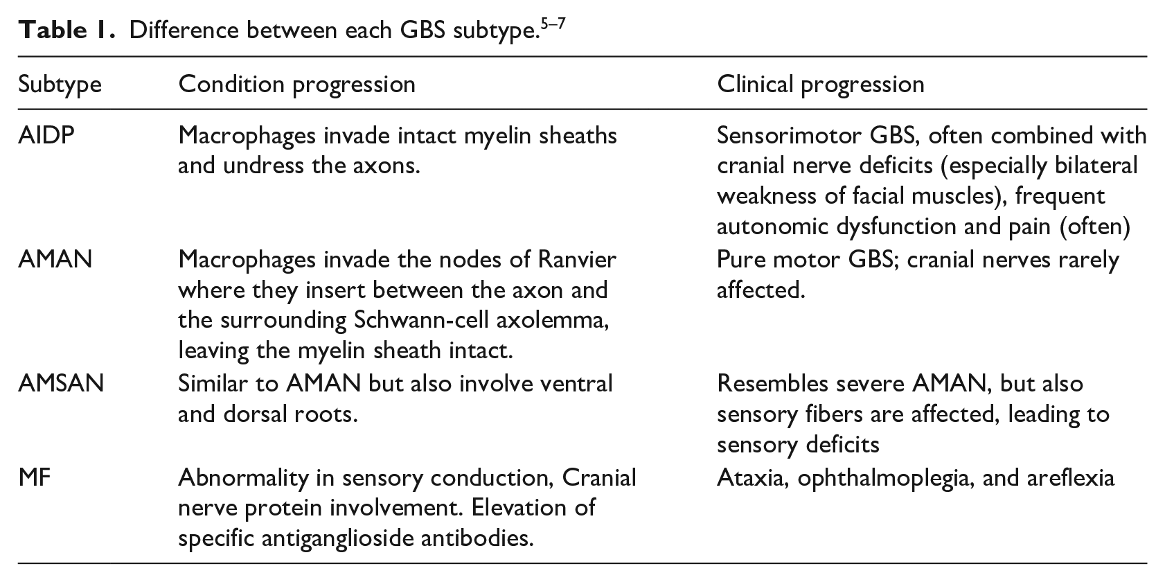
Guillain-Barré syndrome (GBS) is an autoimmune system disorder that affects the peripheral nerves and their roots. It is the most common cause of flaccid paralysis, causing rapid weakness of the facial, respiratory, and swallowing muscles and limbs.¹ GBS is commonly triggered by multifocal inflammation of the spinal roots and peripheral nerves. In severe cases, the prolongation of neurons responsible for driving the nerve impulse is also damaged.² The estimated annual incidence of GBS is 0.61–2 cases per 100,000 people and approximately 25% of patients with GBS require intensive care. Despite adequate supportive treatment, 3.5% die because of complications related to respiratory muscle paralysis, heart attack, or thrombosis.³ This syndrome differs in terms of their appearance, duration, the symmetry of clinical manifestations and if they mainly damage myelin, axon, or mostly peripheral nerve fibers that are dedicated to the motor, sensory and autonomic functions. Therefore the GBS is divided into subtypes, of which four are the most common: acute inflammatory demyelinating polyneuropathy (AIDP), acute motor axonal neuropathy (AMAN), and acute motor.⁴ Due to the variation in severity and treatment between sensory axonal neuropathy (AMSAN) and Miller-Fisher Syndrome (MF) subtypes, differentiation between them is crucial. Table 1 shows the difference between each GBS subtype.

Table 1.

Difference between each GBS subtype.^5
–7

Subtype	Condition progression	Clinical progression
AIDP	Macrophages invade intact myelin sheaths and undress the axons.	Sensorimotor GBS, often combined with cranial nerve deficits (especially bilateral weakness of facial muscles), frequent autonomic dysfunction and pain (often)
AMAN	Macrophages invade the nodes of Ranvier where they insert between the axon and the surrounding Schwann-cell axolemma, leaving the myelin sheath intact.	Pure motor GBS; cranial nerves rarely affected.
AMSAN	Similar to AMAN but also involve ventral and dorsal roots.	Resembles severe AMAN, but also sensory fibers are affected, leading to sensory deficits
MF	Abnormality in sensory conduction, Cranial nerve protein involvement. Elevation of specific antiganglioside antibodies.	Ataxia, ophthalmoplegia, and areflexia

One way to differentiate groups or subgroups in medicine today is through machine learning by creating predictive models. Machine learning is a technique that allows us to build a computational model that learns automatically, this model is then used to simulate and study the behavior of the variables under study. Thus, publications with clinical prediction models have increased in recent years.⁸ For example,⁹ identified and reviewed some of the machine learning and data mining applications in diabetes research as prediction and diagnosis, diabetic complications, genetic background and environment, and health care and management. They found that 85% of machine learning algorithms used a supervised learning approach¹⁰ reviewed the importance of machine learning in the prediction and diagnosis of cancer, using supervised learning techniques such as Artificial Neural Networks (ANNs), Bayesian Networks (BNs), Support Vector Machines (SVM), and Decision Trees (DTs)¹¹ compared different machine learning algorithms such as SVM, Decision Tree (C4.5), Naive Bayes (NB), and k-Nearest Neighbors (k-NN) for the prediction and diagnosis of breast cancer; obtaining the best accuracy with the SVM model¹² employed supervised learning techniques to diagnose Parkinson’s disease and discriminate against Progressive Supranuclear Palsy patients, obtaining an efficiency of approximately 90%¹³ applied a semi-supervised and self-advice learning model to diagnose skin cancer using labeled and unlabeled data. Their model was tested with 100 dermoscopic images and the classification outperformed the most popular methods used in machine learning¹⁴ developed a machine learning model for the diagnosis of glaucoma. Their dataset included 399 cases for training and validation, and 100 cases for testing. Four different algorithms were applied: C5.0, Random Forest (RF), SVM, and k-NN, reaching more than 90% of performance in its results. Despite all the work done in developing prediction models in chronic diseases, there is little literature regarding work with the GBS. The diagnosis and prediction models efficiently improve the detection and classification of diseases. In particular, the diagnosis of GBS is complicated due to a large number of intervening variables.

Previously, diagnosis models for GBS have been created using machine learning algorithms and using the common variables reported in the literature,^15,16 obtained a performance higher than 0.90% in the classification of GBS subtypes in a predictive model based on simple learning algorithms. They conducted experiments with 15 single classifiers in two scenarios and using a dataset with 16 relevant features out of an original 365 feature dataset. In this case, 4 of the 16 features were clinical, and the remaining features came from medical studies. Also,¹⁷ in a predictive model based on the ensemble methods Boosting, Bagging, C5.0, RF, and Random Subspace, reached an accuracy of 0.9366.

In this work, we considered only clinical variables for the creation of our models. Our goal was to investigate if using only the clinical variables could create a diagnosis model for GBS with significant acceptable accuracy. The advantage of having a purely clinical model is that the variables used are detected in medical consultation without the need for complementary studies. We aimed at simplifying previous diagnosis models.

For experiments, we applied four classifiers with different approaches: C4.5 (tree-based), SVM (kernel-based), JRip (rules-based), and k-NN (instances-based). In order to investigate if feature selection can increase the model’s accuracy, we also used filters and wrapper methods. Five filters were selected: Chi-squared, CFS (Correlation-based Feature Selection), Consistency, OneR, and Random Forest. These filters evaluate the goodness of the features based on their intrinsic characteristics in a fast and simple way instead of based on the predictive model; this lead to detect which features are relevant for classification. Then, we choose six wrappers: GA (Genetic Algorithm), Random search, SFS (Sequential Forward Search), SBS (Sequential Backward Search), SFFS (Sequential Floating Forward Search), and SFBS (Sequential Floating Backward Search). The last four wrappers are Deterministic forward or backward search. Wrappers use a predictive model that scores feature subsets based on the error rate of the model, and produce the best selection of features in each iteration. Finally, the One versus All (OvA) binarization technique was used. We compared the balanced accuracy of each created model, where 4 models include all the features, 44 models were obtained using feature selection, and the remaining 16 models were obtained using OvA. Typical metrics evaluated the performance of the models in machine learning such as accuracy, balanced accuracy, sensitivity, specificity, Kappa statistic, and the receiver operating characteristic curve (ROC). Our main metric was balanced accuracy, since our dataset is imbalanced. We used the Wilcoxon non-parametric test¹⁸ to find a statistical difference between the two best models. The two best models including all the features, the two models including only the relevant ones and the two best models with Ova technique.

This article is organized as follows: In section 2, we present a description of the dataset, the machine learning algorithms, and the performance measures used in the study. Section 3 describes the experimental procedure. In section 4, we present and discuss the experimental results. Finally, in section 5, we summarize the results, draw conclusions from the study, and suggest future work.

Materials and methods

Dataset

The dataset used in this work was collected at the Instituto Nacional de Neurología y Neurocirugía (National Institute of Neurology and Neurosurgery) in México from 1993 to 2002. There are 129 patient records, each 1 classified with a kind of GBS subtypes: 20 AIDP, 37 AMAN, 59 AMSAN, and 13 Miller-Fisher. The original dataset has 365 features of which the first 38 are considered clinical; the other 327 correspond to laboratory tests, treatment, and patient tracking. Serological and neuroconduction studies confirmed the subtypes in each patient in this dataset.¹⁹ From the 38 clinical features, 13 were discarded because they represent metadata, such as case number, file number, hospital admission date, discharge date, and duration in days of different situations, leaving the 25 relevant clinical features shown in Table 2.

Table 2.

Dataset features used in this work.

Variable	Feature name	Feature type
v4	Age	✓
v7	Days from the onset of muscle strength diminishing or cranial nerve compromise to the previous event	✓
v9	Days from the onset of symptoms to seek medical advice	✓
v10	Days from the onset of respiratory distress	✓
v36	How many days required the breathing machine	✓
v5	Sex	Male = 1, Female = 2
v21	Weakness	Yes = 1, No = 2
v23	Paresthesia (feeling of tingling, burning skin)	✓
v34	Dyspnea (respiratory distress)	✓
v35	Required assisted ventilation	✓
v2	Diagnosis meets criteria	Range from 1 to 5
v6	Previous event pathology	Range from 0 to 5
v22	Symmetry	Range from 0 to 2
v24	Upper limb muscle strength (strength in arms)	Range from 1 to 6
v25	Lower limb muscle strength (strength in legs)	✓
v26	Location of symptom onset	Range from 1 to 7
v27	Reflexes	Range
v29	Affectation of extraocular muscles	Range from 0 to 2
v30	Ptosis (drooping eyelid - cranial nerve III-)	Range from 0 to 3
v31	Cerebellar affectation	✓
v32	Ataxic gait (cerebellar ataxic gait)	Range from 1 to 3
v33	Cranial nerve involved	Range from 0 to 9
v37	Complications	Range from 0 to 8
v38	Involvement of sphincter (urinary and rectal)	Range from 0 to 2
vS	Season (spring, summer, fall, and winter)	Range from 1 to 4

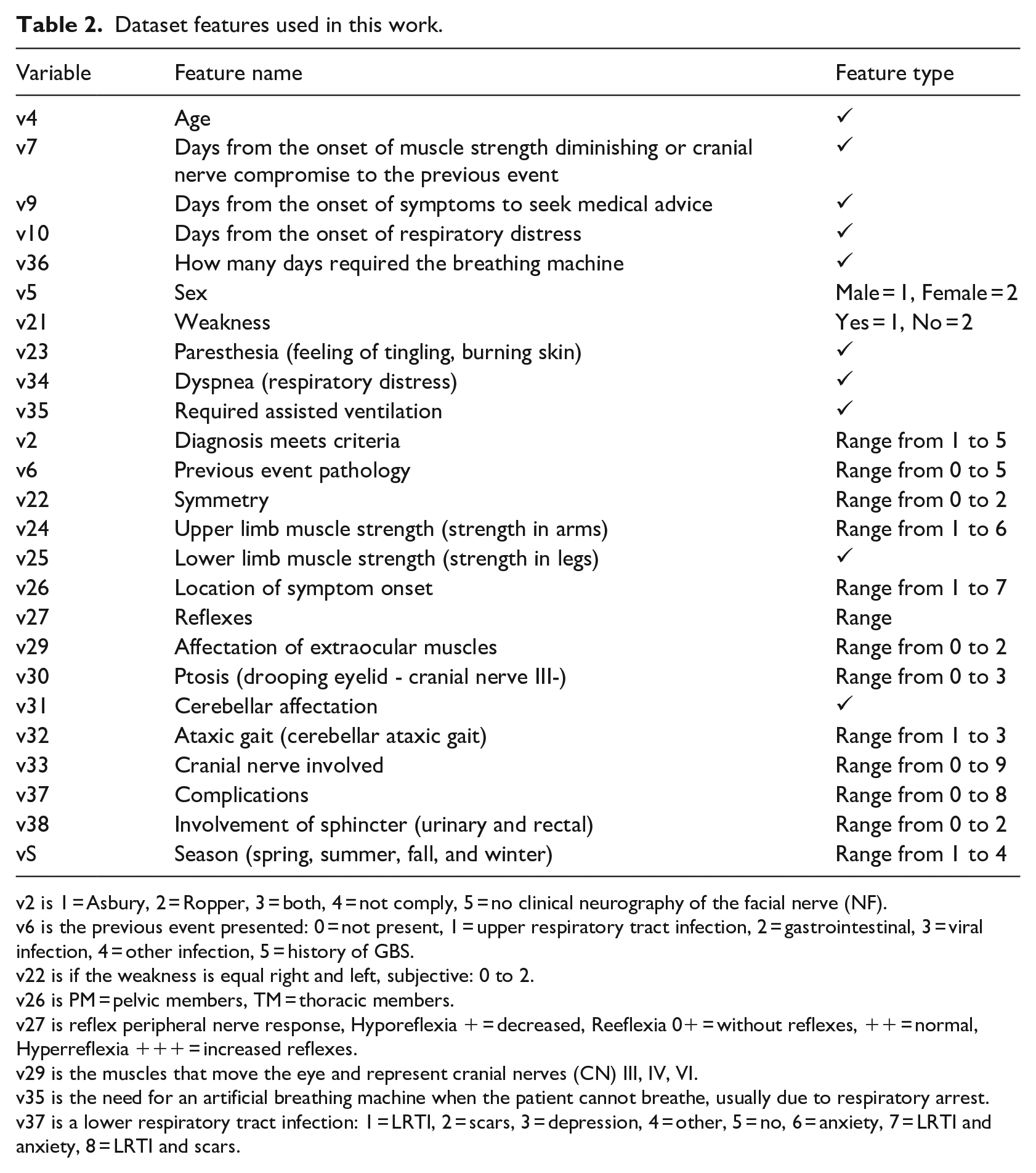
v2 is 1 = Asbury, 2 = Ropper, 3 = both, 4 = not comply, 5 = no clinical neurography of the facial nerve (NF).

v6 is the previous event presented: 0 = not present, 1 = upper respiratory tract infection, 2 = gastrointestinal, 3 = viral infection, 4 = other infection, 5 = history of GBS.

v22 is if the weakness is equal right and left, subjective: 0 to 2.

v26 is PM = pelvic members, TM = thoracic members.

v27 is reflex peripheral nerve response, Hyporeflexia + = decreased, Reeflexia 0+ = without reflexes, ++ = normal, Hyperreflexia +++ = increased reflexes.

v29 is the muscles that move the eye and represent cranial nerves (CN) III, IV, VI.

v35 is the need for an artificial breathing machine when the patient cannot breathe, usually due to respiratory arrest.

v37 is a lower respiratory tract infection: 1 = LRTI, 2 = scars, 3 = depression, 4 = other, 5 = no, 6 = anxiety, 7 = LRTI and anxiety, 8 = LRTI and scars.

Machine learning algorithms

JRip

A ruled-based learner that implements the Repeated Incremental Pruning to Produce Error Reduction (RIPPER) algorithm. JRip identifies the classes by building a set of rules.²⁰ A rule has the form:

if attribute1 <relational operator>

value1 <logical operator>

attribute2 <relational operator>

value2 . . . then

decision-value

C4.5

Builds a decision tree from training data using recursive partitions. In each iteration, C4.5 selects the attribute with the highest gain ratio as the attribute from which the tree is branched,²¹ resulting in a more simplified tree. C4.5 is a decision tree algorithm.

k-NN

Classifies by categories the untagged instances based on the majority class in the k-nearest neighbour in the training set. The classifier’s performance depends significantly on the distance metric used.²²

SVM

Given a set of training instances (input space), where the instances belong to class A or class B, SVM uses a mapping function (kernel) to transform the input space into a dimension space upper (feature space).²³ That is, if the input space is 2D, then it is assigned in a 3D space. In the feature space, SVM finds a hyperplane that gives the most significant separation between classes, called a maximum margin hyperplane. The maximum margin hyperplane has the most significant distance from the hyperplane to the closest training instances. Instances located on the boundaries of the hyperplane are called support vectors. However, the more considerable margin is not always the best solution since it can jeopardize the model’s generalization to new instances. SVM introduces a parameter C that creates a soft margin that allows some errors in the classification, but at the same time penalizes them. An adjustment procedure is necessary to find the best value of C.

Feature selection

The feature selection method allows feature reduction, removing them to increase, or improve the performance. There are three kinds of feature selection: Filter, Wrappers, and Embedded. In this work, we will use the first two.²⁴

Filters

Five filters were taken from the Fselector package: CFS (using correlation and entropy measures), Consistency (using consistency measure), Chi-squared (based on a chi-squared test), OneR (based on simple association rules involving only one attribute in condition part), and Random Forest (using the Random Forest algorithm).²⁵ The first two filters find a feature subset for discrete and continuous data, the remaining ones find weights of discrete attributes.

Wrappers

Six wrappers were taken from the mlr package: GA (genetic algorithm optimization method), Random search (where feature vectors are randomly created, up to a maximum number of features), SFS, SBS, SFFS, and SFBS (extending [forward] or shrinking [backward] a feature set).²⁶

One-versus-all

OvA is a powerful technique and is conceptually simple. OvA turns multiclass classification into binary classification, comparing one class with all the remaining ones.²⁷

Performance measures

Performance measures are a set of statistical techniques, created to describe the performance of models. Different sets of performance measures are applied to the single-label predictors and multi-label predictors.²⁸

Balanced accuracy

Avoids inflated performance estimates in unbalanced datasets. It is the arithmetic mean of sensitivity and specificity or the average precision obtained in any of the classes.²⁹ It is considered more precise than the accuracy when the dataset is unbalanced.

Balanced accuracy = \frac{(\frac{T P}{(T P + F N)}) + (\frac{T N}{(F P + T N)})}{2}

Validation

The validation set approach we used for experiments was a train-test, a straightforward method. We divided two-thirds of the data for the training fitted to the model and one-third for testing and predicting.³⁰

Experimental design

From the dataset described in section Dataset, 64 diagnosis models were created employing the four selected classifiers: 4 diagnosis models using all the features, 44 models using subsets of features obtained after applying filters and wrappers, and 16 models were created using OvA.

For each diagnosis model, we made 30 executions with different seeds to approximate a normal distribution, taking the balanced accuracy as the main metric in each case. For the models with classifiers k-NN and SVM, a pre-execution tuning was performed.

Regarding filters, CFS and Consistency provide a list of the most relevant features when executed, creating a subset of the original dataset. With these two subsets we performed the 30 executions with different seeds. Chi-squared, OneR, and Random forest give a feature ranking as a result, i.e., a ranking of the listed features from most to least relevant. We picked the two best attributes, the three best features from these rankings, and so on until we picked them all. We created subsets with each selection to find which subset of features gives the best performance. This evaluation was performed with 30 independent runs using each classifier.

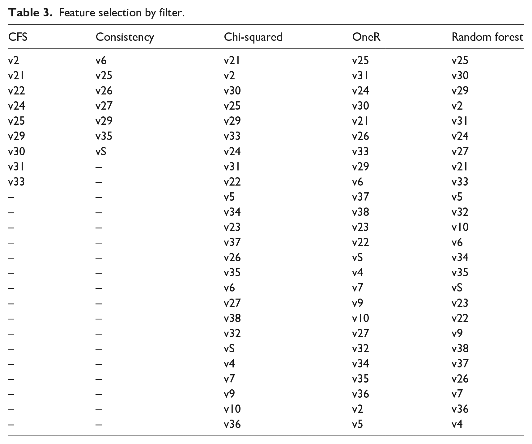
Results for Chi-squared are shown in Figure 1(a), for OneR in Figure 1(b), and Random forest in Figure 1(c). Table 3 shows the feature selection of CFS and consistency filters and the ranking of the Chi-squared, OneR, and Random forest filters.

Figure 1.

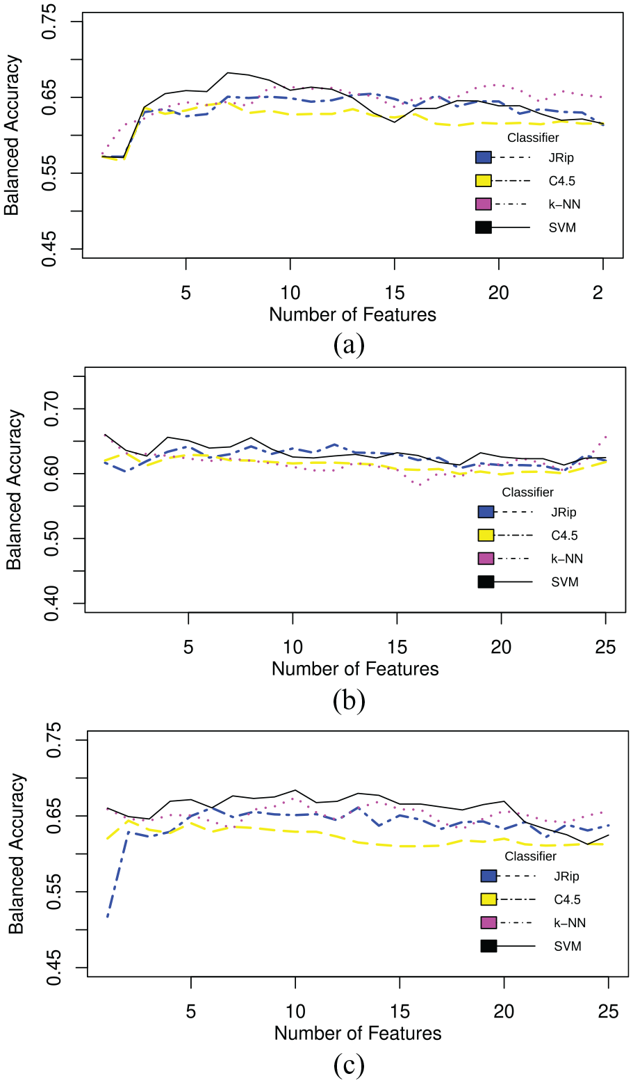
Balanced accuracy across 30 runs: (a) Chi-squared filter, (b) OneR filter, and (c) random forest.

Table 3.

Feature selection by filter.

CFS	Consistency	Chi-squared	OneR	Random forest
v2	v6	v21	v25	v25
v21	v25	v2	v31	v30
v22	v26	v30	v24	v29
v24	v27	v25	v30	v2
v25	v29	v29	v21	v31
v29	v35	v33	v26	v24
v30	vS	v24	v33	v27
v31	–	v31	v29	v21
v33	–	v22	v6	v33
–	–	v5	v37	v5
–	–	v34	v38	v32
–	–	v23	v23	v10
–	–	v37	v22	v6
–	–	v26	vS	v34
–	–	v35	v4	v35
–	–	v6	v7	vS
–	–	v27	v9	v23
–	–	v38	v10	v22
–	–	v32	v27	v9
–	–	vS	v32	v38
–	–	v4	v34	v37
–	–	v7	v35	v26
–	–	v9	v36	v7
–	–	v10	v2	v36
–	–	v36	v5	v4

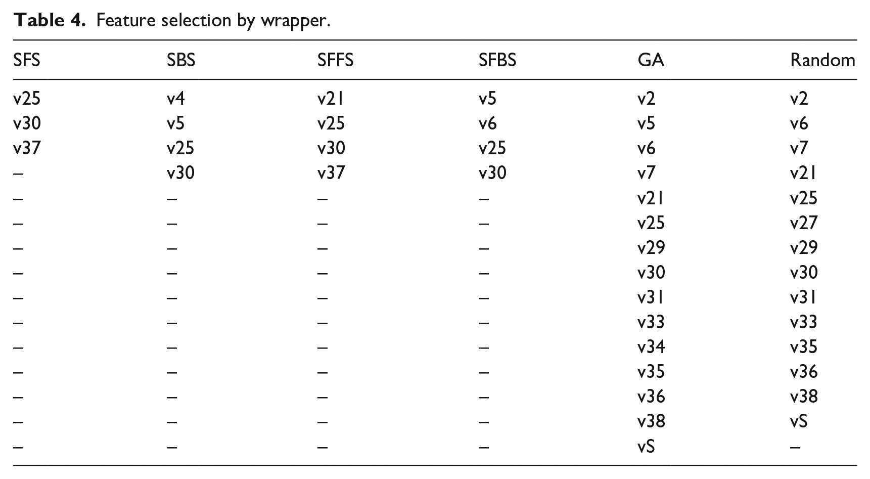
On the other hand, wrappers create a new subset with some features collected with the particular search type, whether Random search, GA, forward, or backward search. These new subsets were tested in each of the selected classifiers. Table 4 shows the chosen feature subset by wrapper.

Table 4.

Feature selection by wrapper.

SFS	SBS	SFFS	SFBS	GA	Random
v25	v4	v21	v5	v2	v2
v30	v5	v25	v6	v5	v6
v37	v25	v30	v25	v6	v7
–	v30	v37	v30	v7	v21
–	–	–	–	v21	v25
–	–	–	–	v25	v27
–	–	–	–	v29	v29
–	–	–	–	v30	v30
–	–	–	–	v31	v31
–	–	–	–	v33	v33
–	–	–	–	v34	v35
–	–	–	–	v35	v36
–	–	–	–	v36	v38
–	–	–	–	v38	vS
–	–	–	–	vS	–

In the case of OvA, we turned the multiclass problem into a binary problem, comparing one GBS subtype against the remaining three. The new datasets AIDP versus ALL, AMAN versus ALL, AMSAN versus ALL, and MF versus ALL were tested in each of the selected classifiers.

A Wilcoxon statistical test was conducted to compare the two best models using all features for detecting all the subtypes, and the two best models using a feature selection method. We used a significance value of 0.05. Similarly, we applied the Wilcoxon test on the two best models for the detection of a subtype with One versus All technique. We used a non-parametric test because the initial conditions that guaranteed the credibility of parametric tests could not be met, making the statistical analysis less reliable with this type of test.

Experiments using the R platform were performed in RStudio 1.1.463; we use the psych, Rweka, Fselector, caret, pROC, rJava, partykit, kknn, randomForest, and e1071 packages.

SVM and k-NN were optimized through the tune function, assigning the values of 0.001, 0.01, 0.1, 1, 10, 50, 80, and 100 for the C parameter in SVM, and the values 5–35 for k, distance 1 for Manhattan, and distance 2 for Euclidean in k-NN.

Results and discussion

Clinical variables are a group of variables used for the diagnosis of GBS. In the literature, all machine learning models include clinical variables plus complementary studies. The Instituto Mexicano del Seguro Social (Mexican Institute of Health) classifies GBS symptoms and signs in three types: typical, additional, and alarm.² The IMSS states that the Asbury and Cornblath criteria are useful for diagnosing conventional forms of Guillain Barré syndrome. The lumbar puncture and electrophysiological studies (the most sensitive and specific diagnostic tests according to³¹ were used to diagnose GBS in the Western Balkans¹. The WHO³ defines GBS cases using the Brighton criteria, which are based on clinical and complementary tests such as neurophysiological studies and lumbar puncture. These diagnostic criteria were validated in another study with a population of 494 adult patients with GBS.³²

In the experiments performed in this work, only clinical variables were used. Table 5 shows the comparison of the best results obtained by each classifier with no filter, the corresponding filters, the average of the 30 executions, the standard deviation, the best, and the worst result. The highest average result obtained by each classifier is highlighted in bold. In Table 5 we can see that in most cases, using filters improves the balanced accuracy, except for Consistency in the JRip and k-NN classifiers.

Table 5.

Comparison of the best results by classifier and filter.

Classifier	Parameters	Balanced accuracy
		All Variables	Chi squared	CFS	Consistency	OneR	Random forest
JRip	Average	0.6265^†	0.6549	0.6463	0.6098	0.6448	0.6606
	SD	0.0459	0.0453	0.0523	0.0436	0.0414	0.0401
	Best	0.7009	0.7336	0.7371	0.7142	0.7120	0.7371
	Worst	0.5426	0.5179	0.5179	0.4557	0.5179	0.5791
C4.5	Average	0.6169	0.6430	0.6321	0.6270	0.6315	0.6438
	SD	0.0599	0.0317	0.0436	0.0266	0.0578	0.0422
	Best	0.6999	0.6934	0.7105	0.6851	0.7173	0.7294
	Worst	0.4828	0.5578	0.5134	0.5544	0.5000	0.5714
k-NN	Average	0.6563^{† *}	0.6668	0.6658	0.6396	0.6590	0.6740^‡
	SD	0.0447	0.0435	0.0540	0.0304	0.0519	0.0371
	Best	0.7337	0.7530	0.7891	0.6859	0.7559	0.7478
	Worst	0.5681	0.5586	0.5121	0.5649	0.5714	0.6084
SVM	Average	0.6254	0.6825	0.6778	0.6298	0.6603	0.6840^‡
	SD	0.0497	0.0486	0.0539	0.0543	0.0458	0.0548
	Best	0.7427	0.7650	0.7960	0.7171	0.7294	0.7798
	Worst	0.5249	0.5915	0.5443	0.4721	0.5544	0.5718

†

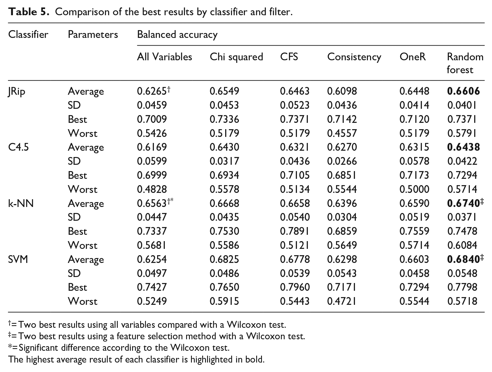
= Two best results using all variables compared with a Wilcoxon test.

‡

= Two best results using a feature selection method with a Wilcoxon test.

= Significant difference according to the Wilcoxon test.The highest average result of each classifier is highlighted in bold.

For the two best models with all the variables for detecting all subtypes (denoted by † in Table 5), the best results were obtained using the k-NN classifier with a balanced accuracy of 0.6563 and, in second place, using the JRip classifier with a balanced accuracy of 0.6265. In this case, there was a significant difference according to the Wilcoxon test. For the two best models using a feature selection method (denoted by ‡ in Table 5), first we have the k-NN and SVM applying Random forest as a filter, reaching a Balanced accuracy of 0.6740 and 0.6840, respectively. In this case, there was not a significant difference according to the Wilcoxon test. For the best two models using the OvA technique (denoted by † in Table 7), we reached with the MF subtype and the classifiers k-NN and SVM a Balanced accuracy of 0.8728 for k-NN and a balanced accuracy of 0.8884 for SVM. In these models, we found no significance with the Wilcoxon test.

Table 6 shows the balanced accuracy obtained using wrappers. Again, the SVM classifier achieved the best performance, this time wit GA wrapper. However, results show that using wrappers for feature selection does not improve in comparison with filter selection.

Table 6.

Comparison of the best results by classifier and wrappers.

Classifier	Parameters	Balanced accuracy
		SFS	SFFS	SFBS	SBS	Random	GA
JRip	Average	0.6221	0.6141	0.6389	0.6198	0.6250	0.6301
	SD	0.0292	0.0319	0.0296	0.0253	0.0445	0.0390
	Best	0.6948	0.6662	0.7227	0.7014	0.7108	0.6851
	Worst	0.5621	0.4900	0.5621	0.5621	0.5084	0.5084
C4.5	Average	0.6292	0.6268	0.6324	0.6232	0.6083	0.6165
	SD	0.0279	0.0269	0.0303	0.0389	0.0478	0.0513
	Best	0.7034	0.7034	0.7187	0.7145	0.7101	0.6948
	Worst	0.5802	0.5596	0.5795	0.5468	0.4854	0.4978
k-NN	Average	0.6443	0.6245	0.6523	0.6525	0.6159	0.6363
	SD	0.0303	0.0447	0.0439	0.0380	0.0377	0.0371
	Best	0.7231	0.7224	0.7332	0.7038	0.6949	0.7105
	Worst	0.5863	0.5510	0.5777	0.5572	0.5151	0.5743
SVM	Average	0.6486	0.6432	0.6483	0.6501	0.6531	0.6584
	SD	0.0392	0.0441	0.0479	0.0490	0.0435	0.0382
	Best	0.7324	0.7324	0.7426	0.7352	0.7387	0.7407
	Worst	0.5729	0.5286	0.5377	0.5509	0.5724	0.5521

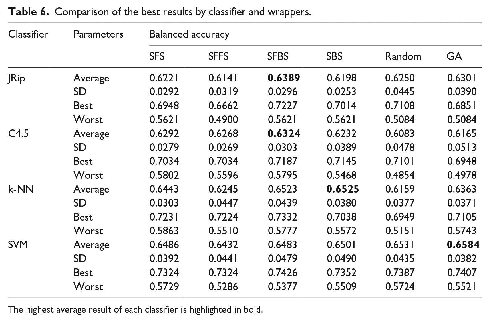
The highest average result of each classifier is highlighted in bold.

One versus All (OvA) classification was applied on the four classifiers to all variables, i.e., with no feature selection method. OvA means that one subtype is compared versus the remaining ones. AIDP versus All, AMAN versus ALL, AMSAN versus ALL, and MF versus ALL. The best result was obtained with SVM classifier and OvA Classification comparing Miller Fisher subtype versus All, reaching a balanced accuracy of 0.8884%. This is mainly due to that Miller-Fisher syndrome (MF) is considered the most common variant of Guillain-Barré syndrome and is characterized by the clinical triad: ophthalmoplegia, ataxia, and areflexia.³³ These clinical variables are represented in our work as the features v27, v30, and v32. Then, we can say that using only clinical variables, it is possible to identify the Miller Fisher GBS subtype from the others. Table 7 shows the average results across 30 runs.

Table 7.

Comparison of the best results by classifier and OvA.

Classifier	Parameters	Balanced accuracy
		AIDP versus ALL	AMAN versus ALL	AMSAN versus ALL	MF versus ALL
JRip	Average	0.5472	0.5394	0.5014	0.8213
	SD	0.0711	0.0542	0.0076	0.1241
	Best	0.7500	0.7167	0.5417	0.9868
	Worst	0.4028	0.4417	0.5000	0.5000
C4.5	Average	0.4995	0.5403	0.5392	0.7259
	SD	0.0093	0.0570	0.0544	0.1336
	Best	0.5278	0.6583	0.6499	0.9868
	Worst	0.4583	0.4000	0.4405	0.4868
k-NN	Average	0.5282	0.6003	0.6190	0.8728^†
	SD	0.0530	0.0530	0.0625	0.1099
	Best	0.6528	0.7083	0.7551	1.0000
	Worst	0.4444	0.4917	0.4760	0.4868
SVM	Average	0.5032	0.5014	0.5600	0.8884^†
	SD	0.0602	0.0076	0.0564	0.0938
	Best	0.6250	0.5417	0.6899	1.0000
	Worst	0.3750	0.5000	0.4497	0.6118

†

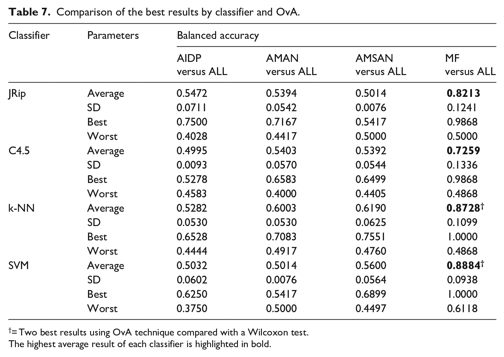
= Two best results using OvA technique compared with a Wilcoxon test.The highest average result of each classifier is highlighted in bold.

Conclusion

In this work, we investigated whether it is possible to create a purely clinical diagnosis model that could quickly and efficiently classify GBS subtypes, through simple classifiers, feature selection by filters and wrappers, and OvA classification. To our knowledge, this work is the first attempt to improve the efficiency of the predictive models of GBS in medical practice.

In this study, we compare the models’ performance with the balanced accuracy parameter. The best performance obtained for the diagnosis of all subtypes was with the SVM classifier and the Random forest filter, achieving a balanced accuracy of 0.6840. But, a performance of 0.8884 with the SVM classifier was reached with the OvA selection on the MF subtype. Currently, our model can be useful for a statistical study of patient records to suggest conclusions and support decision-making.

The results achieved in this study show a significant acceptable accuracy for the diagnosis of one GBS subtypes. Yet, we have not found a way to build a purely clinical model that distinguishes the four subtypes of GBS. Our limitations to achieve such model is that there is no public data about this disease to make comparisons. Also, there are clinical variables often used for diagnosis, e.g., tachycardia, orthostatic hypotension, vasomotor signs, etc. that are not present in our dataset. However, these can only be identified when the condition has progressed.

Serological and neuroconduction studies identified the subtypes suffered by the patients included in the dataset. These studies are not included in this study because our objective was to develop a predictive model that use only variables obtained in clinical practice, in order to help as a primary diagnostic means.

In future works, we consider other techniques to improve the diagnosis through a screening tool in an emergency unit, and for improving the performance of models with solely clinical features. In order to improve our model, we can consider different single classifiers and metaheuristics, ensemble methods, data balancing techniques, and the One versus One (OvO) technique.

Footnotes

Acknowledgements

To CONACYT (Ministry of Science in México) for supporting the Computer Science master’s program at the Universidad Juárez Autónoma de Tabasco.

Conflict of interest

The author(s) declare that there is no conflict of interest.

Funding

The author(s) received no financial support for the research, authorship, and/or publication of this article.

ORCID iD

Oscar Chávez-Bosquez

References

Peric

Milosevic

Berisavac

, et al. Clinical and epidemiological features of Guillain-Barré syndrome in the Western Balkans. J Peripher Nerv Syst 2014; 19(4): 317–321.

Instituto Mexicano del Seguro Social. Diagnóstico y tratamiento: Síndrome de Guillain-Barré, segundo y tercer nivel de atención, http://www.cenetec.salud.gob.mx/descargas/gpc/CatalogoMaestro/089_GPC_SxGBarre2y3NA/GuillainBarrE_EVR_CENETEC.pdf (2016, accessed 15 July 2019).

World Health Organization. Identification and treatment of Guillain-Barré syndrome in the context of the Zika virus outbreak, https://www.who.int/csr/resources/publications/zika/guillain-barre-syndrome/en/ (2016, accessed 16 September 2019).

GBS/CIDP Fundation International. Guillain-Barré syndrome, CIDP and variants: an overview for the layperson, https://www.gbs-cidp.org/wp-content/uploads/2014/09/Overview-for-the-Layperson-ENGLISH.pdf (2010, accessed 07 September 2019).

Panesar

. Guillain-Barré syndrome. US Pharm 2014; 39(1): 35–38.

Uncini

Kuwabara

. Electrodiagnostic criteria for Guillain-Barré syndrome: a critical revision and the need for an update. Clin Neurophysiol 2012; 123(8): 1487–1495.

Van Den Berg

Walgaard

Drenthen

, et al. Guillain-Barré syndrome: pathogenesis, diagnosis, treatment and prognosis. Nat Rev Neurol 2014; 10(8): 469–482.

Steyerberg

. Clinical prediction models: a practical approach to development, validation, and updating. 1st ed. New York: Springer, 2009.

Kavakiotis

Tsave

Salifoglou

, et al. Machine learning and data mining methods in diabetes research. Comput Struct Biotechnol J 2017; 15: 104–116.

10.

Kourou

Exarchos

, et al. Machine learning applications in cancer prognosis and prediction. Comput Struct Biotechnol J 2015; 13: 1–8.

11.

Asri

Mousannif

Al Moatassime

, et al. Using machine learning algorithms for breast cancer risk prediction and diagnosis. Procedia Comput Sci 2016; 83: 1064–1069.

12.

Salvatore

Cerasa

Castiglioni

, et al. Machine learning on brain mri data for differential diagnosis of Parkinson’s disease and progressive supranuclear palsy. J Neurosci Methods 2014; 222: 230–237.

13.

Masood

Al-Jumaily

Anam

. Self-supervised learning model for skin cancer diagnosis. In: 2015 7th International IEEE/EMBS conference on neural engineering (NER), 2015, pp.1012–1015, IEEE Montpellier, France.

14.

Kim

Cho

. Development of machine learning models for diagnosis of glaucoma. PLoS One 2017; 12(5): e0177726.

15.

Hernández-Torruco

Canul-Reich

Frausto-Solís

, et al. Predictores de falla respiratoria y de la necesidad de ventilación mecánica en el síndrome de Guillain-Barré: una revisión de la literatura. Rev Mex Neuroci 2013; 14(5): 162–170.

16.

Canul-Reich

Frausto-Solís

Hernández-Torruco

. A predictive model for Guillain-Barré syndrome based on single learning algorithms. Comput Math Methods Med 2017; 2017: 1–9.

17.

Canul-Reich

Hernández-Torruco

Chávez-Bosquez

, et al. A predictive model for Guillain-Barré syndrome based on ensemble methods. Comput Intell Neurosci 2018; 2018: 1–10.

18.

Cuzick

. A Wilcoxon-type test for trend. Stat Med 1985; 4(1):87–90.

19.

Hernández-Torruco

Canul-Reich

Frausto-Solís

, et al. Feature selection for better identification of subtypes of Guillain-Barré syndrome. Comput Math Methods Med 2014; 2014: 1–9.

20.

Hindle

German

Godfrey

, et al. Automatic classication of large changes into maintenance categories. In: 2009 IEEE 17th International Conference on Program Comprehension, 2009, pp.30–39. IEEE Vancouver, British Columbia, Canada.

21.

Salzberg

. C4.5: Programs for machine learning. Mach Learn 1994; 16(3): 235–240.

22.

Hassanat

Abbadi

Altarawneh

, et al. Solving the problem of the k parameter in the k-NN classifier using an ensemble learning approach. Int J Comput Sci Inf Secur 2014; 12(8): 33–39.

23.

Vapnik

. Statistical learning theory. 1st ed. New Jersey: Wiley-Interscience, 1998.

24.

Keles

Klç

. Artificial bee colony algorithm for feature selection on SCADI dataset. In: 2018 3rd International conference on computer science and engineering (UBMK), 2018, pp.463–466, IEEE.

25.

Romanski

Kotthoff

Schratz

. Package ‘fselector’. CRAN Repository, 2018.

26.

Bischl

Lang

Kotthoff

, et al. mlr: machine learning in R. J Mach Learn Res 2016; 17(170): 1–5.

27.

Rifkin

Klautau

. In defense of one-vs-all classification. J Mach Learn Res 2004; 5: 101–141.

28.

Jiao

. Performance measures in evaluating Machine Learning based bioinformatics predictors for classifications. Quant Biol 2016; 4(4): 320–330.

29.

Witten

Frank

Hall

. Data mining: practical machine learning tools and techniques. 3rd ed. Burlington: Morgan Kaufmann, 2011.

30.

James

Witten

Hastie

, et al. An introduction to statistical learning (with Applications in R), 1st ed. New York: Springer, 2013.

31.

Mendoza-Hernández

Blancas-Galicia

Gutiérrez-Hernández

. Síndrome de Guillain-Barré. Alerg Asma Inmunol Pediatr 2010; 19(2): 56–63.

32.

Fokke

Van Den Berg

Drenthen

, et al. Diagnosis of Guillain-Barré syndrome and validation of brighton criteria. Brain 2013; 137(1): 33–43.

33.

Rodríguez-Uranga

Delgado-López

Franco-Macías

, et al. Síndrome de Miller-Fisher: hallazgos clínicos, infecciones asociadas y evolución en 8 pacientes. Med Clin 2004; 122(6): 223–226.

CFS	Consistency	Chi-squared	OneR	Random forest
v2	v6	v21	v25	v25
v21	v25	v2	v31	v30
v22	v26	v30	v24	v29
v24	v27	v25	v30	v2
v25	v29	v29	v21	v31
v29	v35	v33	v26	v24
v30	vS	v24	v33	v27
v31	–	v31	v29	v21
v33	–	v22	v6	v33
–	–	v5	v37	v5
–	–	v34	v38	v32
–	–	v23	v23	v10
–	–	v37	v22	v6
–	–	v26	vS	v34
–	–	v35	v4	v35
–	–	v6	v7	vS
–	–	v27	v9	v23
–	–	v38	v10	v22
–	–	v32	v27	v9
–	–	vS	v32	v38
–	–	v4	v34	v37
–	–	v7	v35	v26
–	–	v9	v36	v7
–	–	v10	v2	v36
–	–	v36	v5	v4

SFS	SBS	SFFS	SFBS	GA	Random
v25	v4	v21	v5	v2	v2
v30	v5	v25	v6	v5	v6
v37	v25	v30	v25	v6	v7
–	v30	v37	v30	v7	v21
–	–	–	–	v21	v25
–	–	–	–	v25	v27
–	–	–	–	v29	v29
–	–	–	–	v30	v30
–	–	–	–	v31	v31
–	–	–	–	v33	v33
–	–	–	–	v34	v35
–	–	–	–	v35	v36
–	–	–	–	v36	v38
–	–	–	–	v38	vS
–	–	–	–	vS	–

CFS	Consistency	Chi-squared	OneR	Random forest
v2	v6	v21	v25	v25
v21	v25	v2	v31	v30
v22	v26	v30	v24	v29
v24	v27	v25	v30	v2
v25	v29	v29	v21	v31
v29	v35	v33	v26	v24
v30	vS	v24	v33	v27
v31	–	v31	v29	v21
v33	–	v22	v6	v33
–	–	v5	v37	v5
–	–	v34	v38	v32
–	–	v23	v23	v10
–	–	v37	v22	v6
–	–	v26	vS	v34
–	–	v35	v4	v35
–	–	v6	v7	vS
–	–	v27	v9	v23
–	–	v38	v10	v22
–	–	v32	v27	v9
–	–	vS	v32	v38
–	–	v4	v34	v37
–	–	v7	v35	v26
–	–	v9	v36	v7
–	–	v10	v2	v36
–	–	v36	v5	v4

SFS	SBS	SFFS	SFBS	GA	Random
v25	v4	v21	v5	v2	v2
v30	v5	v25	v6	v5	v6
v37	v25	v30	v25	v6	v7
–	v30	v37	v30	v7	v21
–	–	–	–	v21	v25
–	–	–	–	v25	v27
–	–	–	–	v29	v29
–	–	–	–	v30	v30
–	–	–	–	v31	v31
–	–	–	–	v33	v33
–	–	–	–	v34	v35
–	–	–	–	v35	v36
–	–	–	–	v36	v38
–	–	–	–	v38	vS
–	–	–	–	vS	–

Toward a machine learning model for a primary diagnosis of Guillain-Barré syndrome subtypes

Abstract

Keywords

Introduction

Materials and methods

Dataset

Machine learning algorithms

JRip

C4.5

k-NN

SVM

Feature selection

Filters

Wrappers

One-versus-all

Performance measures

Balanced accuracy

Validation

Experimental design

Results and discussion

Conclusion

Footnotes

Acknowledgements

Conflict of interest

Funding

ORCID iD

References

CFS	Consistency	Chi-squared	OneR	Random forest
v2	v6	v21	v25	v25
v21	v25	v2	v31	v30
v22	v26	v30	v24	v29
v24	v27	v25	v30	v2
v25	v29	v29	v21	v31
v29	v35	v33	v26	v24
v30	vS	v24	v33	v27
v31	–	v31	v29	v21
v33	–	v22	v6	v33
–	–	v5	v37	v5
–	–	v34	v38	v32
–	–	v23	v23	v10
–	–	v37	v22	v6
–	–	v26	vS	v34
–	–	v35	v4	v35
–	–	v6	v7	vS
–	–	v27	v9	v23
–	–	v38	v10	v22
–	–	v32	v27	v9
–	–	vS	v32	v38
–	–	v4	v34	v37
–	–	v7	v35	v26
–	–	v9	v36	v7
–	–	v10	v2	v36
–	–	v36	v5	v4

SFS	SBS	SFFS	SFBS	GA	Random
v25	v4	v21	v5	v2	v2
v30	v5	v25	v6	v5	v6
v37	v25	v30	v25	v6	v7
–	v30	v37	v30	v7	v21
–	–	–	–	v21	v25
–	–	–	–	v25	v27
–	–	–	–	v29	v29
–	–	–	–	v30	v30
–	–	–	–	v31	v31
–	–	–	–	v33	v33
–	–	–	–	v34	v35
–	–	–	–	v35	v36
–	–	–	–	v36	v38
–	–	–	–	v38	vS
–	–	–	–	vS	–