
Abstract
Glaucoma is a serious eye disease characterized by dysfunction and loss of retinal ganglion cells (RGCs) which can eventually lead to loss of vision. Robust mass screening may help to extend the symptom-free life for the affected patients. The retinal optic nerve fiber layer can be assessed using optical coherence tomography, scanning laser polarimetry (SLP), and Heidelberg Retina Tomography (HRT) scanning methods which, unfortunately, are expensive methods and hence, a novel automated glaucoma diagnosis system is needed. This paper proposes a new model for mass screening that aims to decrease the false negative rate (FNR). The model is based on applying nine different machine learning techniques in a majority voting model. The top five techniques that provide the highest accuracy will be used to build a consensus ensemble to make the final decision. The results from applying both models on a dataset with 499 records show a decrease in the accuracy rate from 90% to 83% and a decrease in false negative rate (FNR) from 8% to 0% for majority voting and consensus model, respectively. These results indicate that the proposed model can reduce FNR dramatically while maintaining a reasonable overall accuracy which makes it suitable for mass screening.
Introduction
Computer-based diagnosis from image data is important for medicine. Eye images provide an insight into important parts of the visual system and can also indicate the health of the entire human body. Glaucoma is an eye disease that can lead blindness. It is a disease in which structural changes occur to the optic nerve head, retinal nerve fiber layer (RNFL) thickness, and ganglion cell and inner plexiform layers as well as loss of the visual field. 1 The retinal optic nerve fiber layer can be assessed using optical coherence tomography, scanning laser polarimetry (SLP), and Heidelberg Retina Tomography (HRT) scanning methods. However, these methods are expensive and hence a novel automated glaucoma diagnosis model that uses extracted features from digital fundus images is needed. Robust mass screening may help to extend the symptom-free life for the affected patients; the ocular fundus image can be easily obtained and can be used to automatically identify whether an eye is glaucomatous or not. However, the image has a two-dimensional distribution, and it is difficult to feature the whole image through some real-valued parameters in general. 2
Generally, raw datasets usually include useful information that cannot be extracted by traditional data classification; although traditional solutions can reveal some latent information, they often require longer time and usually include some human mistakes. Finding hidden relationships in datasets from different sources (e.g. medical science, transportation, news, social media, weather, . . ., etc.) require computer-based solutions, such as machine learning and data mining 3 to provide reliable worthy models with high accuracy. The exploration of medical data is a significant issue as it has a close direct relationship to our life. Thus, the proposed models in this field should have the lowest error rates in terms of treatment and diagnosis. 4 These popular models and techniques include support vector machine (SVM), Naïve Bayes model, K-Nearest neighbor (KNN), and random forests (RFs).
SVM is a supervised learning algorithm that depends on the statistics theory. It is basically used for dimensional pattern recognition and nonlinear regression. In both cases, sample data are split into two different feature groups: training data that is applied for training the SVM model network and testing data that is used for the model validation. SVM treats all data equally as it requires all the training feature data to be multiplied with the same weighted coefficient, which neglects the importance of the special feature data. Accordingly, fuzzy memberships are used to describe the corresponding input feature data, which is regarded as the affiliation of corresponding feature data to one of the classes. 5
Naïve Bayes algorithm was introduced to the text retrieval community in the 1960s. 6 It is a machine learning tool that depends on applying Bayes’ theorem with strong independence assumptions between the features. Naïve Bayes classifier is a popular method for text categorization that rules if documents do belong to one category or another based on word frequencies as the features. This classifier can solve the problem of multi-class density-based classification. In other words, it can calculate explicit probabilities for each hypothesis based on the Bayes theorem. 7 Although Naïve Bayes algorithm is less competitive than SVM, it was successfully applied in automatic medical diagnosis. 8
KNN is a non-parametric supervised machine learning algorithm that can solve both regression and classification problems. 9 It relies on labeled input data to learn a function that produces an appropriate output when given new unlabeled data. The input consists of the k-closest training examples in the feature space. In KNN classification, the output is a class membership; an object is classified by a plurality vote of its neighbors, with the object being assigned to the most common class among its k nearest neighbors. 10
RFs is a nonlinear regression or classification model that consists of ensembles of regression/classification trees such that each tree depends on a random vector sampled independently from the data. Random forests algorithm was introduced by Breiman 11 to overcome some of the shortcomings of the decision trees algorithm particularly its instability with small perturbations in a learning sample. RFs uses many randomly built decision trees to combine their predictions and reduces the possible correlation between decision trees by selecting different subsamples of the feature space. It turns out that the random forests algorithm has become a very powerful, efficient, and popular tool for the survival analysis. 12
This paper is organized as follows: The following section provides literature review on the use of the above machine learning models and few others to screen glaucoma patients. Section 3 presents the proposed system. Section 4 lays out the experimental results, and finally conclusions are provided in Section 6.
Related works
Several works attempted to help with glaucoma diagnosis. For example, an inductive logic programming (ILP) system called GKS was developed, not only to deal with low-level measurement data such as images, but also to produce diagnostic rules that are readable and comprehensive for interactions with medical experts. 13 Another work provided automated identification of normal and glaucoma classes using Higher Order Spectra (HOS) and Discrete Wavelet Transform (DWT) features. 14 The extracted features are fed into the SVM classifier with linear, polynomial order 1, 2, 3, and Radial Basis Function (RBF) to select the best kernel function for automated decision making. In this work, SVM classifier with kernel function of polynomial order 2 was able to identify the glaucoma and normal images automatically with an accuracy of 95%, and sensitivity and specificity of 93.33% and 96.67%, respectively. Mookiah et al. 14 present a computer-based glaucoma screening system in which optic nerve defects detection, visual field examination, and expert system fuzzy rules are combined to increase the sensitivity and specificity. 14 The system is cost effective and is suitable for detecting early-stage glaucoma, especially for large-scale screening.
Several computational algorithms have been used for image-based glaucoma diagnosis. Most of these methods follow the two-stage pipeline structure: feature extraction and classification. This includes Discrete Wavelet Transform (DWT), Higher Order Spectra (HOS), Gabor transform for feature extraction and SVM, Artificial Neural Network (ANN), and KNN for prediction. The design of such hand-crafted features is a tedious job and time consuming. These features are strongly related to expert knowledge with a restricted representation power. Thus, for a huge dataset it cannot show the discriminative power. Deep features are essential to overcome this problem and enhance the classification performance. Using deep neural network techniques like CNN were applied on colored retinal images and achieved promising results as shown in Raghavendra et al.15,16
The detailed literature reviews of the existing work for automated glaucoma diagnosis are summarized in Table 1. Moreover, the table includes a comparative summary with different performance parameters such as: accuracy (acc), sensitivity (sen), and specificity (spc).
A summary of the existing work for automated glaucoma diagnosis.

GLAUDIA: A predicative system for glaucoma diagnosis in mass scanning
In the following sub-sections, we describe the dataset and the proposed model.
Dataset
The dataset is retrieved from Kim et al. 34 It consists of 499 numerical records with seven input features extracted from digital fundus images and one label feature in a CSV file format. The dataset is distributed as follows: 202 records of non-glaucoma cases and 297 of glaucoma cases (primary open angle glaucoma (POAG) or normal tension glaucoma (NTG)). The dataset contains a set of features that are used to describe the glaucoma cases including age, ocular pressure, cornea thickness, retinal nerve fiber layer (RNFL) thickness, glaucoma hemifield test (GHT), history of macular degeneration (MD), and pattern standard deviation (PSD). In addition to one dependent variable (diagnosis) that takes either a value of 1 to indicate a Glaucoma case or a value of 0 to indicate a normal case. All features are used as an input to the classifiers.
For more information on feature extraction from the dataset, see Kim et al. 34
Proposed model
Figure 1 represents the proposed model, which consists of six steps. In the first step, the data is preprocessed by normalizing the values of each feature to be between 0 and 1 as shown in equation (1). The data is then divided into two sets: 80% for training and 20% for testing as indicated in step 2. Different types of classifiers are applied to the training parts with 10-fold validation to obtain generalized models as shown in step 3. In step 4, we use accuracy from the average of 10-fold divisions to rank the models, where accuracy is defined as the percentage of true predicated cases either positive or negative to the total number of all cases as shown in equation (2).
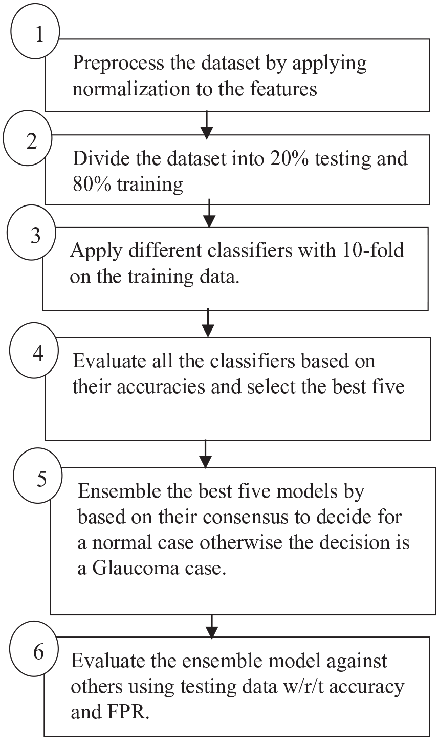
Proposed model.
In step 5, the top five models with the highest accuracy are ensembled together; all the models have to be in consensus about a case to be classified as a negative case (no glaucoma disease), while if one model is positive about a case, then the case will be classified as a positive case (glaucoma disease). The final decision of the stacked model is defined as shown in equation (4). Finally, the proposed model is evaluated with the other staging models that are based on the majority voting, not on the consensus, from two different metrics: accuracy and FNR. Equation (3) shows the FNR that represents the percentage of positive cases (glaucoma disease) that were falsely predicated as negative cases (no glaucoma disease).
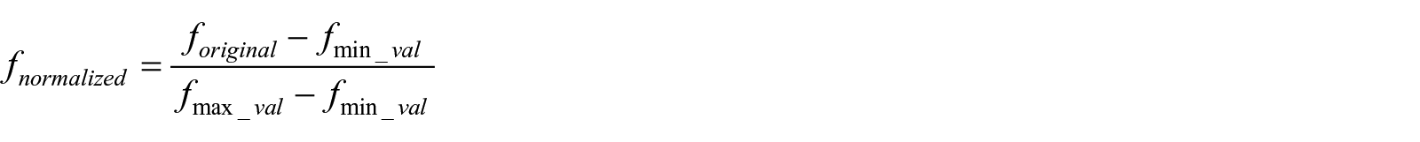
Where

Where:


Experimental results
In this section we describe the results obtained and give a detailed discussion about it. We used the Google Colab (a tool for machine learning) for the implementation of the machine learning techniques, Python and Keras (a machine learning library) were used. We started our experiment by normalizing the data to ensure that it is between 0 and 1. After that, we divided the data into 80% for training and 20% for testing. The division is done using a built-in library in Skit Learn that grants random and balanced distributions of the output labels. It is worth mentioning that the data distribution is 40.4% non-glaucoma cases and 59.6% glaucoma cases; the data is not fully balanced. However, the bias is on the side of positive cases which can be more suitable for mass screening as the goal is to reduce FNR even if this leads to reducing the overall accuracy for the sake of early diagnosis.
In the machine learning step, nine different techniques were applied: Logistic Regression, K-Neighbors, Random Forest, Decision Tree, Naïve Bayes with both Gaussian and Bernoulli distributions, and SVM with different kernels (Linear, Poly, and RBF). For each model, we used 10-fold validation for the training data to grant generalization for the obtained model and to avoid any overfitting by averaging the resulting error from the validation results. In addition, a random search approach for tuning each model parameters were used to achieve best accurate result. Figure 2 shows a bar chart for the mean average accuracy from applying 10-fold validation for the nine models in descending order.
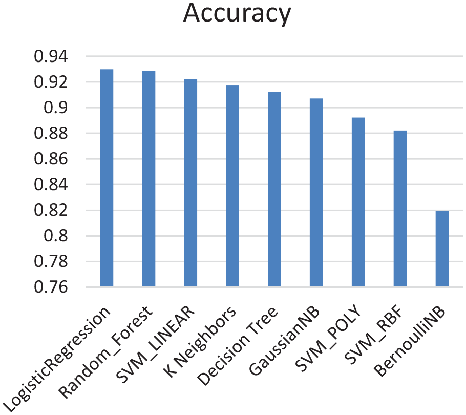
Results obtained from applying machine learning algorithm.
From Figure 2, the highest five accuracies were achieved by Logistic Regression, Random Forests, SVM with linear kernel, K-Nearest Neighbors, and decision trees. We have then built an ensemble model that constitutes these top five models only. We evaluated the model for both majority voting and consensus using 20% of the dataset, that is, to decide if a case is negative, majority voting must have a highest count for a negative case across all the techniques while the consensus model needs just one technique to determine that the case is negative. The consensus among the five models does also help with avoiding overfitting as its target is to reduce false negative error based on reducing the overall accuracy to be suitable for mass scanning.
For the first phase, we chose 10-fold validation to overcome the sample size limitation and avoid any overfitting. While in the second phase we divided the dataset into 80% for training and 20% for testing which is a rule of thumb in dividing small size datasets reasonably.
A comparison between the FNR is shown in Figure 3. The results show that FNR has decreased to 0% using the ensemble model. In Table 2, we compare between the accuracy of the ensemble while considering the majority voting approach and consensus approach, it is noticed that accuracy has decreased from 90% for the majority voting to 83% for the consensus approach.
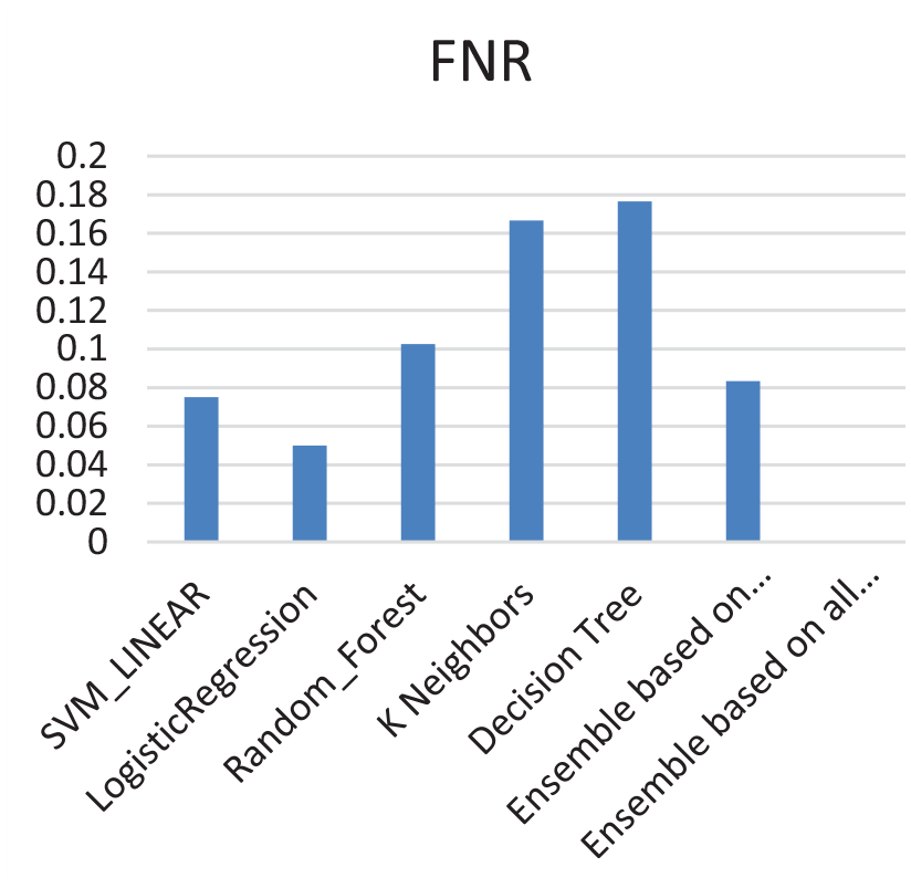
Comparisons of FNR for the best top five models, ensemble based on majority voting, and ensemble based on consensus.
Accuracy of ensemble models.

Conclusions and future work
This paper presents a new model to screen for the glaucoma disease based on different features. The proposed model compares between different machine learning techniques and ensemble the top five techniques that provide the highest accuracies based on 10-fold validation. The ensemble of the best top five models is done via two different approaches: majority voting and consensus. The results obtained a decrease in the accuracy from 90% using majority voting to 83% using consensus for testing data that was never seen before by the trained models. The results also show a decrease in false negative rate (FNR) from 8% using majority voting to 0% using consensus. When it comes to mass screening, FNR is more critical than accuracy as the main goal is to reduce the number of cases that needs to be screened by the physicians to positive cases only. This makes the ensemble approach based on consensus an attractive one. The main contribution of this work is to identify five top best classifiers based on the resulting accuracy rate, in addition to providing a consensus model that aims to reduce the false negative rate to make the proposed model more suitable for mass scanning. Future work includes combining different modalities to diagnose glaucoma, such as retinal images associated with risk factors to increase the accuracy of the model without losing the advantage of having low FNR, in addition to differentiating between Glaucoma types. In addition, other features that do not exist in the current dataset would be considered, such as gender and race as they might have a role in Glaucoma diagnosis.