Sage Journals: Discover world-class research

Abstract

Early and accurate diagnoses of sepsis enable practitioners to take timely preventive actions. The existing diagnostic criteria suffer from deficiencies, such as triggering false alarms or leaving conditions undiagnosed. This study aims to develop a clinical decision support system to predict the risk of sepsis using tree augmented naive Bayesian network by identifying the optimal set of biomarkers. The key feature of our approach is that we captured the dynamics among biomarkers. With an area under receiver operating characteristic of 0.84, the proposed model outperformed the competing diagnostic criteria (systemic inflammatory response syndrome = 0.59, quick sepsis-related organ failure assessment = 0.65, modified early warning system = 0.75, sepsis-related organ failure assessment = 0.80). The richness of our proposed model is measured not only by achieving high accuracy, but also by utilizing fewer biomarkers. We also propose a left-center-right imputation method suitable for electronic medical record data. This method uses the individual patient’s visit, instead of aggregated (mean or median) value, to impute the missing data.

Keywords

artificial intelligence Bayesian classifiers clinical decision support system data mining machine learning sepsis

Introduction

Sepsis is a life-threatening organ dysfunction caused by a dysregulated host response to infection.¹ Patients with sepsis are at considerable risk of severe complications and death. In-hospital mortality rates for sepsis patients range from 10% to 20%.² Between 2007 and 2013, the number of hospital admissions due to sepsis increased nearly 49% to more than 352 per 1,00,000 persons per year.³ At about $20 billion, or 5.2% of national hospital costs, sepsis is considered the most expensive condition treated in U.S. hospitals.⁴

The prognosis of sepsis is a complicated process due to its complex physiological mechanism. The complication involves the effect of individual variables as well as the random variations. A proper understanding of dynamics among variables is important to explain the state of the disease. Recently, the new definition of sepsis has been introduced by Sepsis-3 in an effort to simplify the diagnosis of sepsis.¹ This definition proposed a paradigm shift by moving the focus of sepsis diagnoses from inflammatory response to organ failures. The Sepsis-3 study also tied the diagnosis of sepsis in suspected infected patients to the risk of mortality.⁵

Most of the existing sepsis diagnostic criteria still rely on the old definitions and lack in performance: systemic inflammatory response syndrome (SIRS) are known to have poor specificity,^6–8 modified early warning system (MEWS) have limited accuracy,⁹ and sepsis-related organ failure assessment (SOFA) are highly complex and require knowledge of four laboratory results that can be difficult to measure in resource constrained environment.¹⁰ Although a new diagnostic criteria, known as quick sepsis-related organ failure assessment (qSOFA), was proposed with the announcement of new sepsis definitions, it was not widely accepted in medical communities due to its poor sensitivity.¹¹ Hence, there exists a need for a diagnostic model that is easy to use and delivers high performance.

Bayesian network modeling techniques, with their characteristic to capture the conditional dependencies among variables, can be suitable to describe the relationship among biomarkers for the better prediction of mortality. Bayesian networks are very popular for capturing the uncertain knowledge in medicine and have been extensively used in the diagnosis of diseases.^12–14 The tree augmented naive (TAN) Bayesian network is a specific class of Bayesian networks used for classification problems and applied widely in health care.¹⁵ The TAN Bayesian networks perform better than alternate classifiers when biomarkers are correlated, and at the same time maintain the mathematical simplicity.^16,17

In this article, we developed a clinical decision support system to predict the risk of sepsis using TAN Bayesian network. Following the Sepsis-3 study, the main hypothesis of our study is that mortality and sepsis have a close relationship among patients with suspicion of sepsis. Therefore, we used mortality to infer about the diagnosis of sepsis. The framework to develop the model includes the following steps: data preprocessing, model learning, and evaluation. The data preprocessing phase includes imputation, variable selection and discretization. In the model learning phase, the interactions among selected biomarkers were captured by utilizing the TAN Bayesian network. Unlike other studies where biomarkers were considered independently,¹⁸ our study captured probabilistic interactions among biomarkers to better estimate the risk of mortality. Finally, along with discussing results with practitioners, the performance of the proposed model was compared to popular diagnostic criteria used in practices such as SIRS,¹⁹ qSOFA,¹ MEWS²⁰, and SOFA.²¹ Our predictive model outperforms existing sepsis diagnostic criteria while using fewer biomarkers.

This study makes the following contributions:

Develop a sepsis predictive model with high sensitivity and high specificity by utilizing the new sepsis definitions.

Identify important biomarkers that enable easy and quick diagnosis.

Capture probabilistic interrelations among biomarkers rather than considering them independent to better evaluate the risk of mortality.

Propose an imputation method that is suitable for electronic medical records where percentage of missing data is dominant.

The remainder of the article is organized as follows. “Literature review” section includes a synopsis on relevant studies. “Method” section discusses data, preprocessing of data, and applied methodology along with an explanation of the proposed imputation approach. “Results and discussion” section includes the comprehensive set of experiments. “Conclusion” section elaborates on the results and incorporates concluding remarks.

Literature review

Many studies have been dedicated to the development of decision support systems for sepsis identification to aid practitioners in diagnosis. Mathe et al.²² developed a sepsis surveillance system that monitors specific lab and vital signs in real time, and visualizes them on a screen. The system notifies health care providers in case of observed abnormalities. However, this tool does not analyze the information recorded and provide any suggestion about the future outcome. Brandt et al.²³ derived a flow chart for sepsis diagnosis and developed an electronic sepsis surveillance system. The major drawback of the system was that it had low specificity. Amland and Hahn-Cover²⁴ designed a computerized early warning tool for sepsis diagnosis. This tool generates two kinds of alerts: SIRS alert and sepsis alert. The results showed that the system was able to alert physicians with the median of 8.6 h earlier than the time of suspicion of infection noted by doctors. The limitation of this tool was that it triggered many false-positive alarms. Only 25% of patients that were alerted required the physician’s attention. Henry et al.²⁵ proposed a Target Real-time Early Warning (TREW) score to predict septic shock using the cox-proportional hazard model. This support system triggers a warning of septic shock based on the change in clinical variables over time. The proposed model achieved discrimination ability of 0.83. The limitation of this analysis is that it does not capture the effect of previous condition of disease and also does not comment about the mortality risk. Most expert systems for sepsis consider clinical variables independently. However, it is highly unlikely that physiological variables are independent.

A few attempts have been made to apply Bayesian network to understand the dynamics of sepsis. Mani et al.²⁶ developed a predictive model using noninvasive clinical observations for sepsis prediction among neonatals (infants during the first month). The authors compared the performance of nine machine-learning algorithms and found that naive Bayes, with area under receiver operating characteristic (AUROC) curve of 0.79, outperformed other learning techniques. Gultepe et al.¹² applied the Bayesian network structure learning algorithm (hill-climbing) to unearth the interaction among clinical variables used for sepsis diagnosis. Along with developing the Bayesian network structure to understand the dependencies among variables, the authors also proposed a model for mortality prediction using naive Bayes and support vector machine (SVM). With AUROC of 0.73, SVM-based model performed better than naive Bayes. The possible reason for poor performance of naive Bayes model was that the data set was small (number of patients was 741 where only 151 had sepsis and others were of control group). Nemzek et al.²⁷ applied Bayesian networks to the protein and cellular components of sepsis-related organ failure and elucidated the intricate relationships among the variables that cause lung dysfunction. Although this study provided detailed insights on development of sepsis-related lung dysfunction, it used the protein and cellular components that are not directly accessible and required laboratory analysis.

Some studies use the variant of Bayesian networks known as dynamic Bayesian networks (DBNs) to improve the performance of sepsis diagnostic system. Peelen et al.¹³ proposed a clinical support system for medical practitioners to predict organ failures in intensive care units (ICUs). They developed three different models of the problem, and each model is an advancement of the previous. Model 1 takes into account the number of organ failures, Model 2 considers the transition of one organ failure to other, and Model 3 incorporates the dependency of one organ failure to other organs, that is, independent assumption was relaxed. The authors captured the dynamic nature of patients’ recovery in ICU using a Markov chain. The states in the Markov chain denote various conditions of patient’s stay in the ICUs. The transition probabilities are calculated using logistic regression. The limitation of the study is that the authors used data only from ICU admissions; therefore, it was not clear to what extent the findings could be generalized to non-ICU admissions. Another study by Sandri et al.²⁸ developed a model to predict the sequence of organ failure in a patient using DBNs. The main limitation of this study was that the organ dysfunctional time was not known, therefore, authors used orders of organ failure based on physicians’ recommendations.

In this study, we capture important interactions among biomarkers. The inclusion of dynamics among biomarkers differentiates our model from existing models. In addition, the existing sepsis diagnostic models lack in providing balance between sensitivity and specificity.^6,11 Due to the nature of unbalance between sensitivity and specificity, both qSOFA and SIRS were criticized and considered unhelpful. Therefore, practitioners require a more sophisticated diagnostic system. MEWS provides a better alternative, but its sensitivity, specificity, and AUROC are not strong. Although SOFA provides high performance accuracy, its complexity is the biggest challenge in resource-constrained environments.¹⁰ In this article, we aim to develop an easy-to-use expert system using Bayesian network classifier that captures the interaction among clinical variables and facilitates a balance between sensitivity and specificity by selecting the optimal set of biomarkers.

Method

In this study, we used the following steps to build a predictive model: (1) data extraction, (2) data preprocessing (imputation, feature selection, and discretization), and (3) building TAN Bayesian network (Figure 1).

Figure 1.

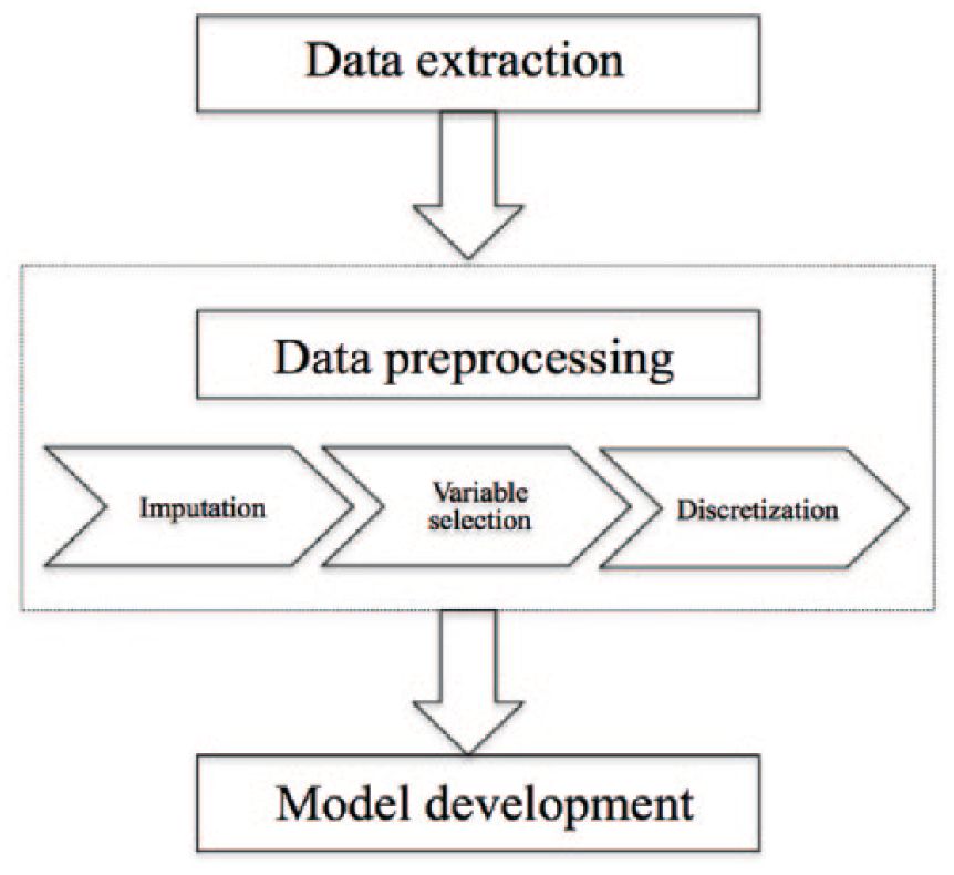
Systemic procedure to develop model.

Data extraction

This study used deidentified data from Cerner Corporations HIPAA-compliant Health Facts database. The database comprises electronic health records (EHRs) for 379 million patient visits, about 63 million patients, from 480 affiliated hospitals across the United States. These comprehensive clinical records for individual patient visits include demographic, vital signs, laboratory results, medication, diagnosis codes (both ICD-9 and ICD-10), pharmacy, procedures performed, and date- and time-stamped information on admission and discharge. This data set is one of the largest electronic medical records in the United States.²⁹

The population of suspected infection was selected using the gold standard explained in Sepsis-3.⁵ The gold standard includes a combination of culture drawn (Event 1) and antibiotics administration (Event 2) within a defined time interval. There are two scenarios: (1) Event 1 occurs first, then Event 2 occurs within 72 h, (2) Event 2 occurs first, then Event 1 occurs within 24 h. The study cohort includes patient visits that satisfy either of the two aforementioned scenarios. The time of infection is the time of occurrence of the first event. The selection of culture and antibiotic was based on the consultation with practitioners. In the final data set, we had 16,909 patient visits. The outcome variable was discharge type (expired or nonexpired).

Data preprocessing

Data preprocessing includes three main steps. First, the missing values in the data were imputed using the proposed left-center-right method. Second, an optimal set of variables was identified using feature extraction, and these variables were used for further construction of the model. Using the combination of elastic net and recursive partitioning, irrelevant, or redundant variables were eliminated. Third, the selected biomarkers were discretized using Hartemink³⁰ method, which is suitable to be used with Bayesian classifiers.

Imputation

This section explains the proposed left-center-right imputation method and compares it to alternate imputation approaches. Imputation is a critical step to develop an effective clinical model using EHR data. EHR data are collected for the billing purpose rather than performing analytics, therefore, the data have a lot of missing clinical measurements. Also, variables that are easy to measure such as routine vital signs are frequently present while others, such as lab tests, are sparsely available. Since we wanted to capture the interactions among variables, it was important to use values recorded in the same time intervals instead of taking the aggregate values such as mean or median over the hospital stay of the patient. Considering measurements at the same time interval is especially important for sepsis as it progresses aggressively, therefore, aggregate measurements are clinically less meaningful.

In the proposed imputation method, we utilized observed biomarker measurements to impute unobserved biomarkers of individual patient’s visit. For this study, we divided the patient’s length of stay after the first suspicion of infection into 24 h (or 1 day) windows. We selected 24 h windows because the popular existing criteria such as SOFA uses the worst value recorded in 24 h.²¹ The imputation procedure is easy to explain with the example shown in Figure 2. In Figure 2, t = 0 is the time at which patient is suspected to have infection. The subsequent hospital stay is divided into 24 h intervals until the discharge of the patient (i.e. t = 8). 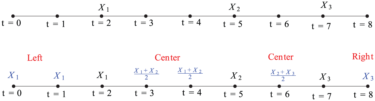For a specific variable in a patient visit, suppose we know the observation for t = 2, 5, and 7 ( $X_{1}$ , $X_{2}$ , and $X_{3}$ ). To impute the values in remaining intervals, we use carry-forward (right in Figure 2) and carry-backward (left in Figure 2) methods along with the mean in intermittent intervals (center in Figure 2). In the carry-forward and carry-backward methods, the most recent value is carried forward or backward, respectively, to fill empty intervals. We referred to this imputation method as left-center-right for convenience. Using observed data at t = 2, 5, and 7 (shown in black), the other time intervals were imputed (shown in blue).

Figure 2.

Left-center-right imputation.

We compared the imputed data generated from the proposed imputation method to the mean and the median imputation. This comparison was established for each individual variable. For illustration purposes, let us consider bilirubin. The same population data (explained in “Data extraction” section) were used for this comparison purpose. We expect that good imputed data should follow the density plot of data without imputation. Figure 3 shows the density plot of three imputation techniques along with density plot of data without imputation. The density plot for the left-center-right method closely aligns with the data without imputation as desired. The density plots obtained from other imputation techniques changed the shape of distribution and showed peaks at different points than the original mean. The reason for peaks at different points is attributed to the sparsity of EHR data. Therefore, we avoided the use of mean or median imputation for our analysis.

Figure 3.

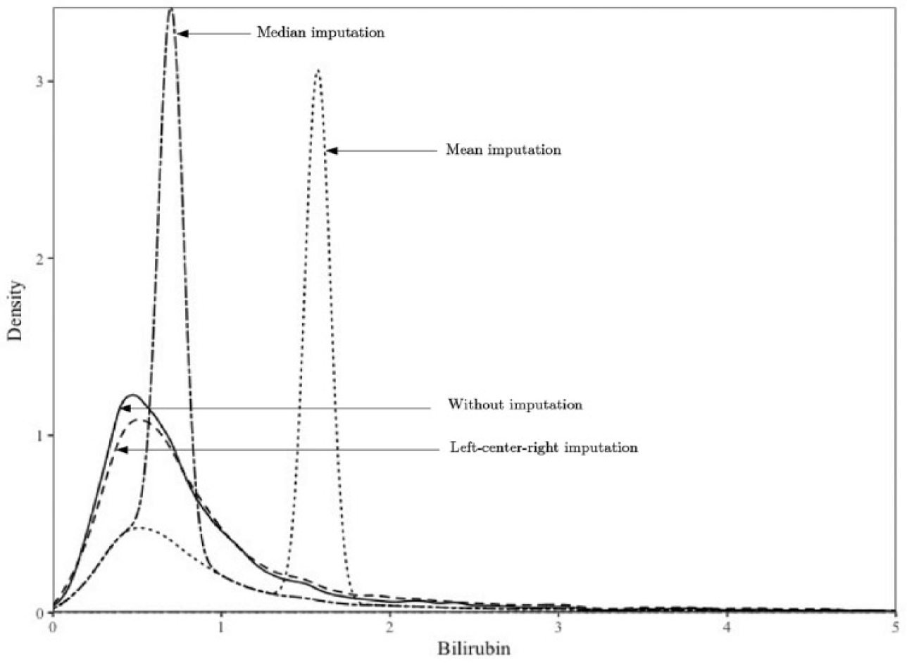
Density plots for different imputation techniques.

Variable selection

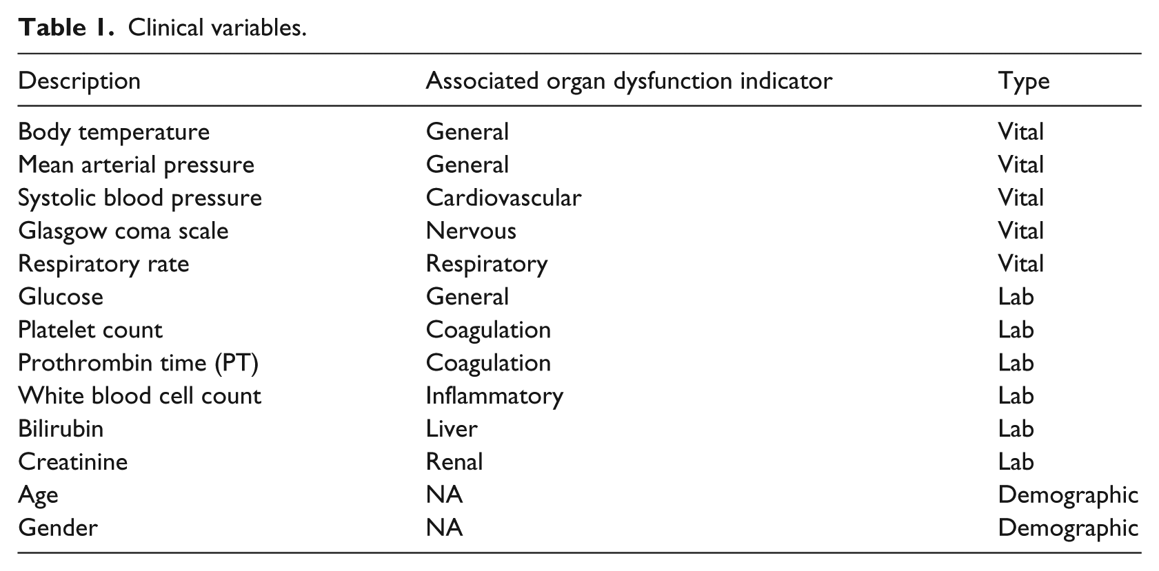
Variable selection is the most critical part of the analysis because most clinical results have lead time and cost associated with it. Also, Capan et al.³¹ has shown that not all organ failures are equally associated with sepsis mortality. Therefore, to keep our model simple, and at the same time maintain high performance, we need to establish the best subset of variables. Table 1 includes the names and types of the variables initially selected in this study. The primary selection of biomarkers was based on the literature and discussion with practitioners. Later, the best subset of biomarkers among the primarily selected biomarkers was obtained using the machine learning techniques.

Table 1.

Clinical variables.

Description	Associated organ dysfunction indicator	Type
Body temperature	General	Vital
Mean arterial pressure	General	Vital
Systolic blood pressure	Cardiovascular	Vital
Glasgow coma scale	Nervous	Vital
Respiratory rate	Respiratory	Vital
Glucose	General	Lab
Platelet count	Coagulation	Lab
Prothrombin time (PT)	Coagulation	Lab
White blood cell count	Inflammatory	Lab
Bilirubin	Liver	Lab
Creatinine	Renal	Lab
Age	NA	Demographic
Gender	NA	Demographic

We used both elastic net³² and recursive partitioning³³ for variable selection. The two methods stand on different principals. The elastic net pulls the coefficients of unimportant variables toward zero by minimizing the sum of square errors and regularization term. We used the elastic net rather than the stepwise selection because it facilitates shrinkage and avoids overfitting using the regularizing factor. The shrinkage implies reducing the complexity of the model by dragging the weights of unimportant biomarkers to zero. Shrinkage is an important characteristic for clinical applications because each biomarker (lab test or vital signs) is associated with a significant cost. The recursive partitioning focuses on minimizing the impurity present in the data by partitioning. For the final model, a conservative approach was applied and only variables that were suggested by both variable selection methods were used.

Zou and Hastie³² proposed elastic net regression that utilized both L1 norm and L2 norm. The objective function (or prediction error) for the elastic net is given by equation (1). The variable of interest is the weight vector at which objective function is minimum

\hat{w} = a r g \min_{w} {\sum_{n = 1}^{N} {(Y^{n} - w^{T} X^{n})}^{2} + λ α ∥ w ∥_{1} + \frac{λ (1 - α)}{2} ∥ w ∥_{2}}

(1)

Here $Y^{n}$ is the observed output (discharge type) of $n t h$ data point, $X^{n}$ is the input vector of length $p$ (number of biomarkers; $p$ = 13) of $n t h$ data point, $n$ is the index for admission visit $(n \in {1, 2, \dots, N})$ . $N$ is the number of admission visits ( $N$ = 16,909). $α$ is a tuning parameter, $w$ is a estimated weight vector, and $∥ w ∥_{1}$ , $∥ w ∥_{2}$ are L1 norm and L2 norm, and equal to $Σ_{j = 1}^{p} | w_{j} |$ and $\sqrt{Σ_{j = 1}^{p} w_{j}^{2}}$ , respectively. For a specific $α$ , we search for best $λ$ that provides the least cross-validation error (CV-E) with the minimum set of biomarkers.

To obtain an optimal set of variables, we searched for different $α$ $(0 \leq α \leq 1)$ and $λ$ . Figure 4 shows the plot between CV-E and $\log (λ)$ on different $α$ . Five-fold cross-validation was used to avoid the bias due to selection of sample. Each dot (in red) and bar (in gray) in the graph represents the CV-E and one standard deviation from mean, respectively, corresponding to a specific $\log (λ)$ . Two vertical lines in each plot represent $λ$ at which CV-E is minimum and $λ$ above which CV-E is greater than one standard deviation of the minimum CV-E. To compute the optimal number of variables, we used $λ$ above which CV-E is greater than one standard deviation of the minimum CV-E instead of using $λ$ at which CV-E is minimum. This selection of $λ$ enables significant reduction in the size of optimal set of variables with the minimal increase in error. For example, at $α$ = 1, minimum CV-E was achieved at $\log λ$ = –7.32 with 12 variables (shown in the top of each plot) and maximum CV-E that is within one standard deviation of minimum CV-E is at $\log λ$ = –5.27 with nine variables. Therefore, we selected nine as an optimal set of variables for $α$ = 1. We expected as $α$ decreases, sparsity of the model decreases due the nature of equation (1). It is evident from Figure 4 that the optimal number of variables increases as $α$ decreases from 1 to 0. The size of optimal set of variables for $α$ = 0.33 and $α$ = 0 were 10 and 13, respectively (bottom two plots of Figure 4). Figure 4 depicts number of selected variables on the top of each plot. This number of selected variables is identified using variables with nonzero weights. The clinical variables with zero weights for $α$ = 0.66 and log( $λ$ ) = –4.3 are struck out in Table 2.

Figure 4.

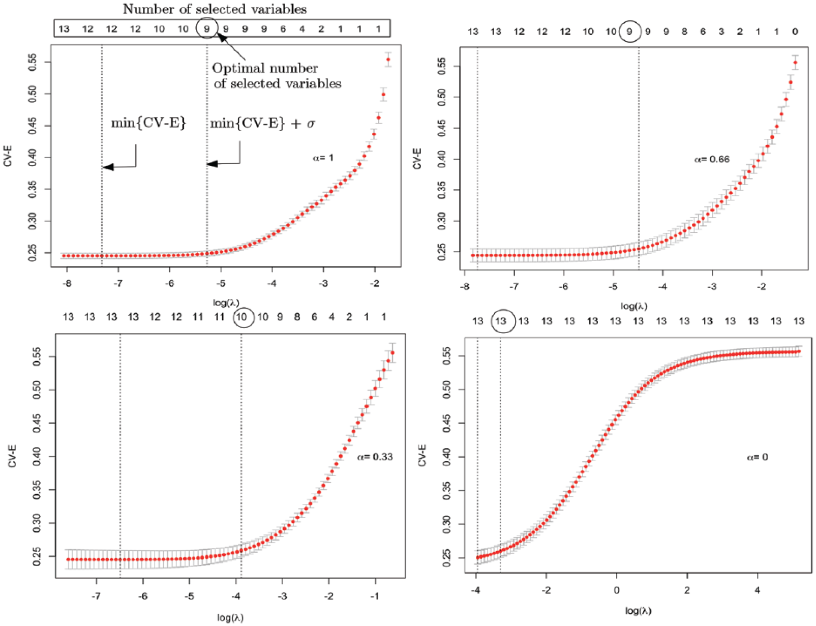
CV-E versus $\log (λ)$ on $α$ = 1, 0.66, 0.33, 0.

Table 2.

Variable weights for $α$ = 0.66 and log( $λ$ ) = –4.3.

Variable	Variable
Body temperature	Prothrombin time (PT)
Mean arterial pressure	White blood cell count
Systolic blood pressure	Bilirubin
Glasgow coma scale	Creatinine
Respiratory rate	Age
Glucose	Gender
Platelet count

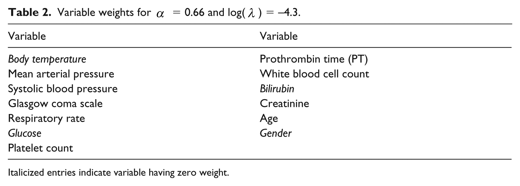
Italicized entries indicate variable having zero weight.

In recursive partitioning, the data are recursively partitioned to reduce the impurity present in the data. Each step of the recursive partitioning includes the splitting of data into two subgroups. The split is determined by the variable that reduces the impurity most. We used two methods to measure the impurity: Gini index and Information index.³³

Gini index is defined as

G i n i i n d e x = \sum_{i = 1}^{2} p_{i} (1 - p_{i})

Information index is defined as

I n f o r m a t i o n i n d e x = - \sum_{i = 1}^{2} p_{i} l o g (p_{i})

Where $p_{i}$ is the probability of outcome class $i$ . We have two classes in outcome variable (1 = nonexpired, 2 = expired).

The recursive partitioning can be summarized as follows:

1. Select variable that provides highest information gain (or reduction in impurity). The information gain is calculated using the following expression

Information gain = impurity (before split) - impurity (after split)

2. Split data using the selected variable.

3. Repeat 1 and 2 until information gain is greater than a predefined threshold.

For our data, recursive partitioning using both splitting criteria resulted in the same classification accuracies (0.96). Since we had the same classification accuracies and the research has shown that both criteria disagree only in 2% cases,³⁴ we selected information index for further explanation of the results.

The variable importance of each biomarker obtained by recursive partitioning using information index is shown in Figure 5. Figure 5 illustrates a significant drop in variable importance from respiratory rate (RR) to mean arterial pressure. Therefore, we performed a sensitivity analysis to inspect the change in accuracy for two scenarios: considering only first five important variables (dotted variables in Figure 5), considering all variables with nonzero variable importance. The classification accuracy of the model (0.96) with five variables (dotted variables in Figure 5) was the same as the classification accuracy of the model (0.96) with nine variables (both dotted and shaded variables in Figure 5). Therefore, we considered only five biomarkers from recursive partitioning: Glasgow coma scale (GCS), creatinine, blood pressure, white blood cell (WBC), and RR.

Figure 5.

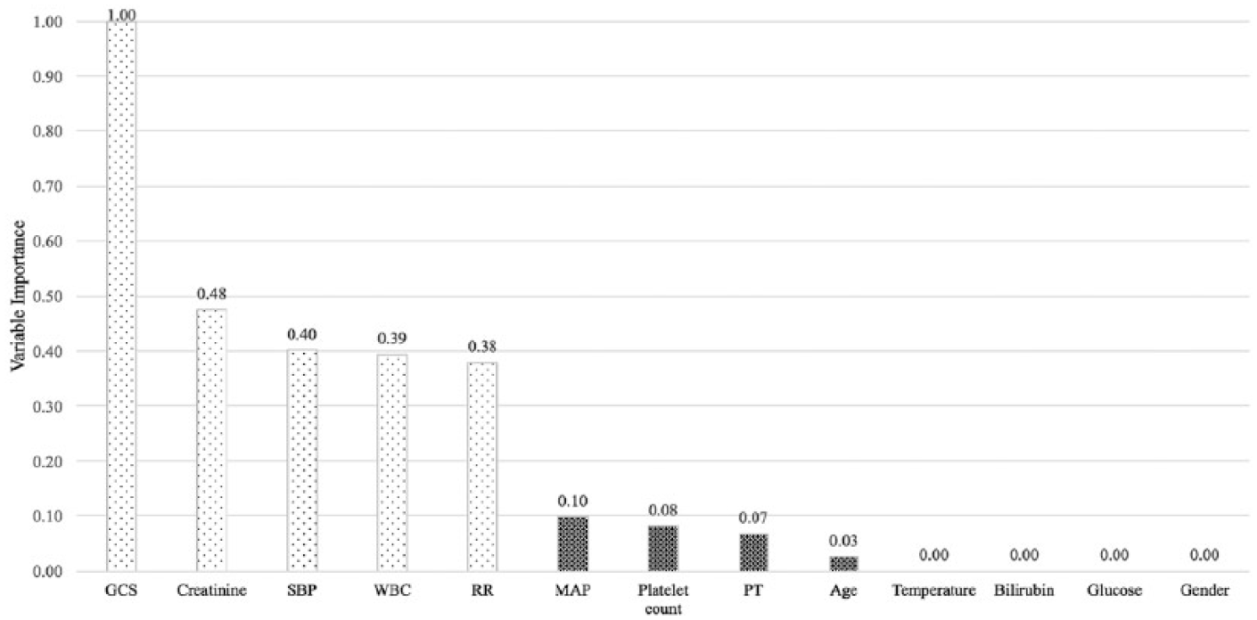
Variable importance from recursive partitioning.

We summarized the variables selection using elastic net ( $α$ = 0, 0.33, 0.66, 1) and recursive partitioning in Table 3. Although for our experiments, the variables, selected by recursive partitioning, are the subset of variables selected by the elastic net ( $α$ = 1), it is not always the case. The variables used for further analysis are shown in bold font in Table 3.

Table 3.

Selected variable.

Variable	$α$ = 0	$α$ = 0.33	$α$ = 0.66	$α$ = 1	Recursive partitioning
Body temperature	✓
Mean arterial pressure	✓	✓	✓	✓
Systolic blood pressure	✓	✓	✓	✓	✓
Glasgow coma scale	✓	✓	✓	✓	✓
Respiratory rate	✓	✓	✓	✓	✓
Glucose	✓
Platelet count	✓	✓	✓	✓
Prothrombin time (PT)	✓	✓	✓	✓
White blood cell count	✓	✓	✓	✓	✓
Bilirubin	✓	✓
Creatinine	✓	✓	✓	✓	✓
Age	✓	✓	✓	✓
Gender	✓

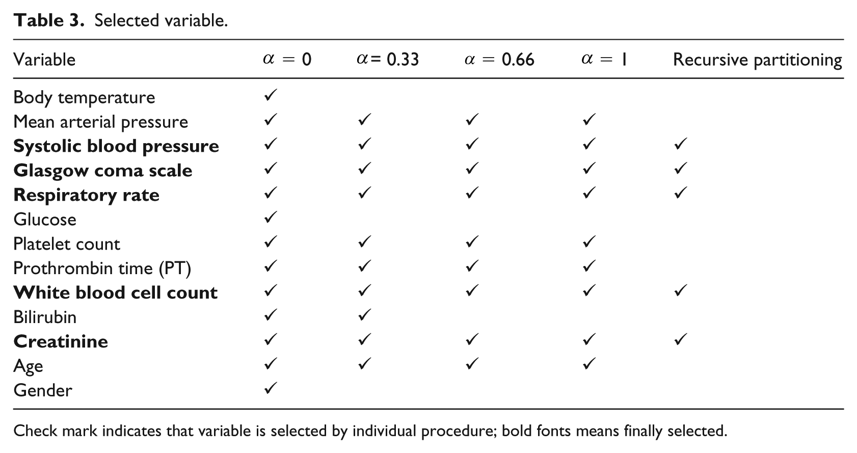
Check mark indicates that variable is selected by individual procedure; bold fonts means finally selected.

Discretization

Many methods have been developed to discretize continuous variables, and the performance of these methods depends on the shape and the nature of the data. Some approaches such as quantile and equal intervals utilize variables in isolation, while others such as Hartemink³⁰ consider relationship among variables to decide the cut-offs.

The correlation analysis uncovers significant dependencies among biomarkers. Figure 6 illustrates correlations among biomarkers. The size of the circle represents the strength of the correlation between biomarkers. The cross signs show that the correlation was nonsignificant. Therefore, a relationship among biomarkers should be utilized for discretization to avoid the loss of information. Hence, we selected Hartemink method to efficiently compute the discrete levels of biomarkers. Another reason why we chose it is that research has shown that Hartemink³⁰ discretization performs better with Bayesian classifiers.

Figure 6.

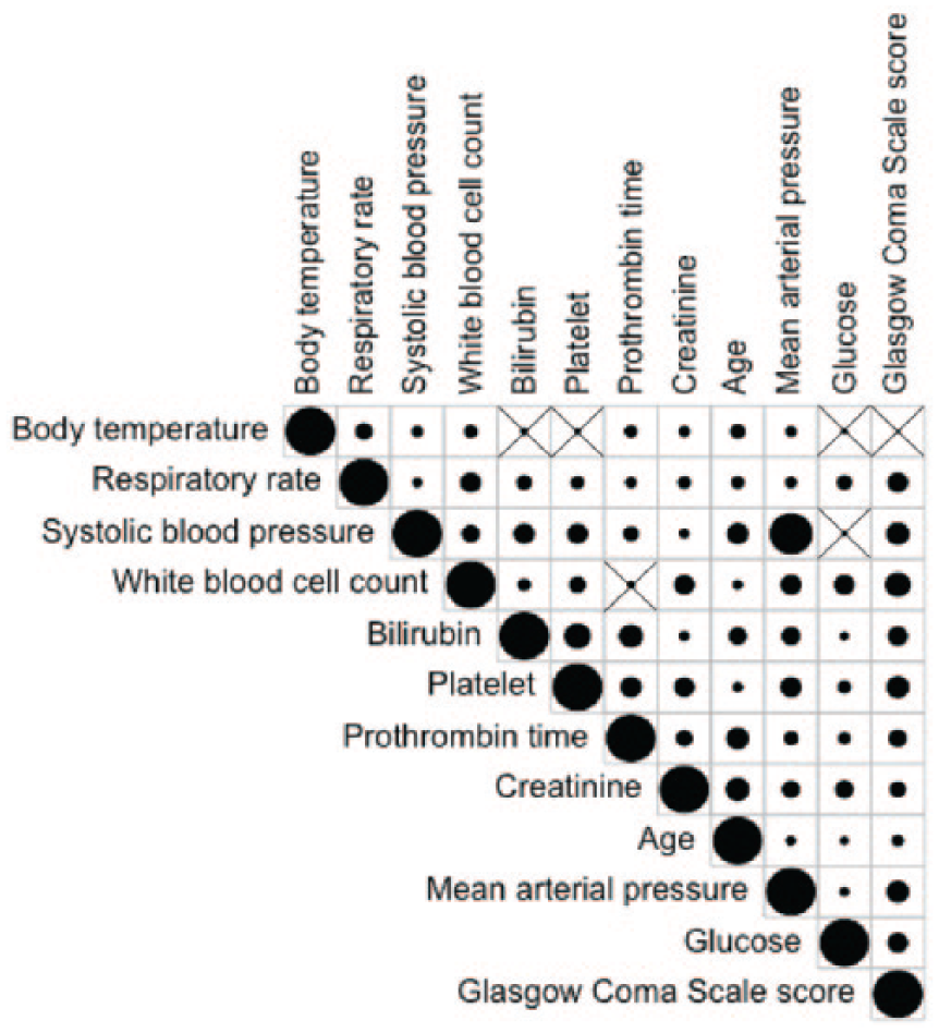
Correlation analysis among biomarkers.

Hartemink discretization assumed that the continuous variables are normal by distribution. Therefore, we inspected the density plot of each variable. Using the Box-Cox method,³⁵ the transformed variables were obtained when original variables were deviating from normal, except for the GCS sore. For example, the original distribution of platelet count and its transformed distribution are shown in Figure 7. The GCS score was heavily left skewed, therefore, no better distribution was found using the Box-Cox method. 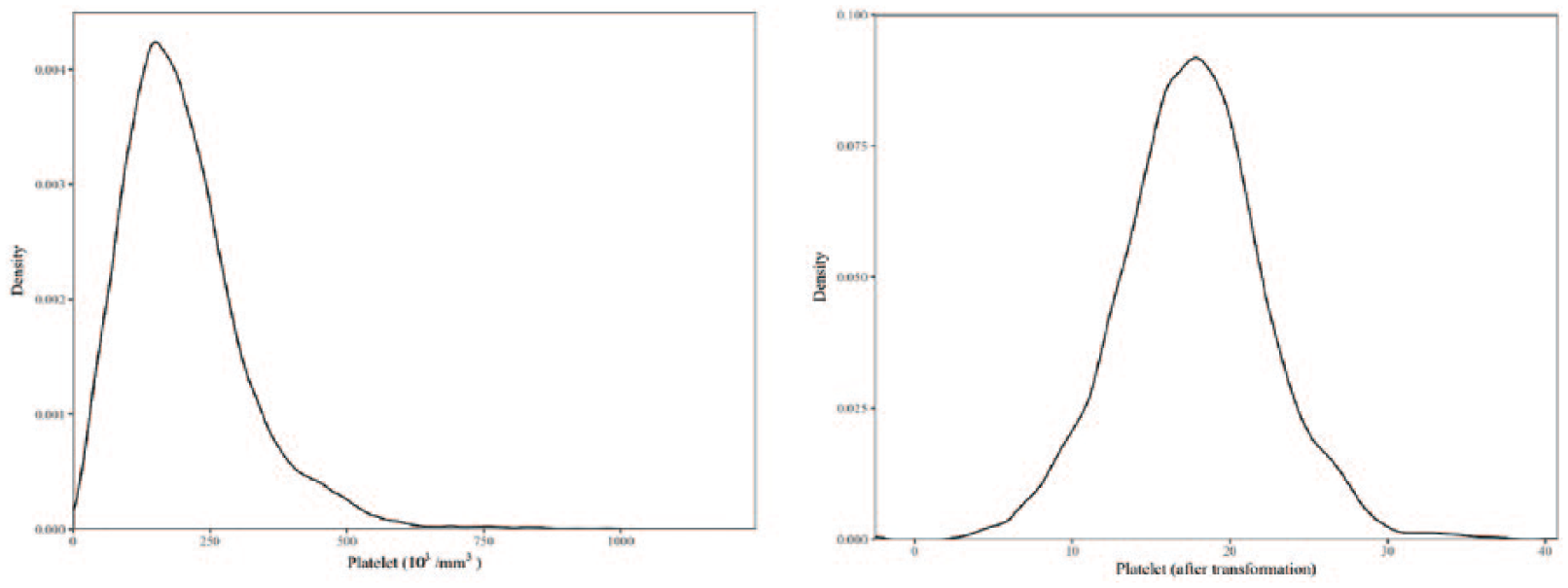Hence, the cut-offs $(\leq 6, (6, 10], (10, 13], > 13)$ defined in the literature were applied for GCS.²¹

Figure 7.

Platelet (before and after transformation).

In the Hartemink method, each continuous variable initially is segregated into a large number of levels using any of the traditional methods such as equal intervals. This large number of levels reduces to a specific number, defined by the users, by coalescing selected neighboring pair to a single level. The mutual information (MI) between the selected variable and other variables is calculated. The levels that result in a minimum loss of information with any of the other variables is coalesced with neighboring level. For our experiments, we first divided each variable into 10 levels and then coalescing was done with the Hartemink procedure until each variable reached three levels. Based on physicians’ opinion, three discrete levels facilitate simplicity and meaningful clinical interpretation. Some biomarkers are considered as normal at mid-range value and as abnormal at either extreme end. The three discrete levels are able to discover the mid-range boundaries.

The computed discrete levels of the selected variables provide important insights. The patterns of mortality over different discrete levels of biomarkers (shown in Figure 8) are supported by practitioner’s knowledge. For example, practitioners suggested that both low and high RRs are associated with increased mortality. The discrete levels obtained from our analysis also showed the same pattern. However, there exists slight differences in the standard cut-offs and cut-offs obtained from discretization. The standard RR for a normal patient is 12 to 20 breaths per minute. However, we obtained least mortality for RR between 16 to 22 breaths per minute. It is possible that generated cut-offs work well for sepsis specifically because the upper cut-off is supported by the recent Sepsis-3 study, where RR greater than 22 was proposed as the cut-off for increased risk of mortality.

Figure 8.

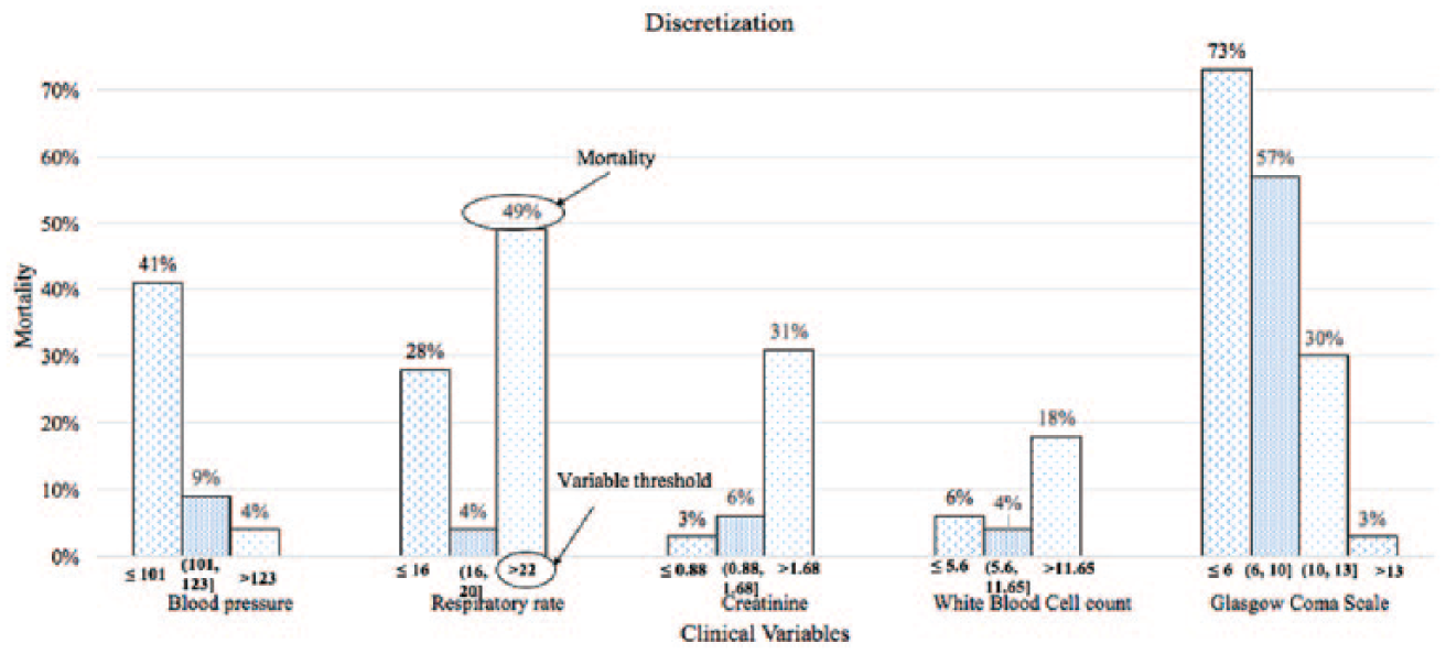
Discrete levels of selected biomarkers and corresponding mortality rate.

Model development

Bayesian network is a probabilistic model with directed acyclic graph. Combination of nodes and arcs is used for the graphical representation. Each node represents a random variable, and each arc implies conditional dependencies between variables. Bayesian networks are popularly used in medical research because they capture the uncertainties and nonlinearities presented in data using graphical representation that is easy to understand.³⁶

There are two popular Bayesian classifiers: Naive Bayesian and TAN Bayesian. The Naive Bayes classifiers are simple and assume conditional independence between variables given the outcome variable. TAN improves Naive Bayes classifier to capture important interactions among variables and at the same time maintains the mathematical simplicity. In TAN, the outcome variable (mortality risk) has no parent, and each predictor can have at most two parents: class variable and any other biomarker. The procedure to learn the structure of the proposed model is explained as follows.³⁷

Step 1: Calculate the MI between each pair of biomarkers using the following equation

M I (X_{i}, X_{j} | Y) = \sum_{k = 1}^{C_{X_{i}}} \sum_{l = 1}^{C_{X_{j}}} \sum_{m = 1}^{C_{Y}} P (k, l, m) \log \frac{P (k, l | m)}{P (k | m) P (l | m)}

(2)

where $C_{X_{i}}$ , $C_{X_{j}}$ , and $C_{Y}$ are the number of levels in variable $X_{i}$ , $X_{j}$ , and $Y$ , respectively. $i$ , $j$ $\in$ {GCS, systolic blood pressure (SBP), RR, WBC, creatinine}.

Step 2: Build a complete undirected graph with the MI as the weight of edges.

Step 3: Find the maximum weighted spanning tree.

Step 4: Transform the undirected tree obtained from Step 3 to a directed one by choosing a root variable either arbitrarily or by expert’s opinion, and setting the direction of all edges to be outward from it. In this study, the selection of root node was performed using an expert’s opinion such that the selection does not violate any domain knowledge. The establishment of direction does not change the data likelihood because MI( $X_{i}$ , $X_{j}$ ) = MI( $X_{j}$ , $X_{i}$ ).

Step 5: Include new node (mortality risk) and connect it with the rest of the graph obtained in Step 4.

The steps to construct TAN Bayesian network for the current sepsis model are shown in Figure 9.

Figure 9.

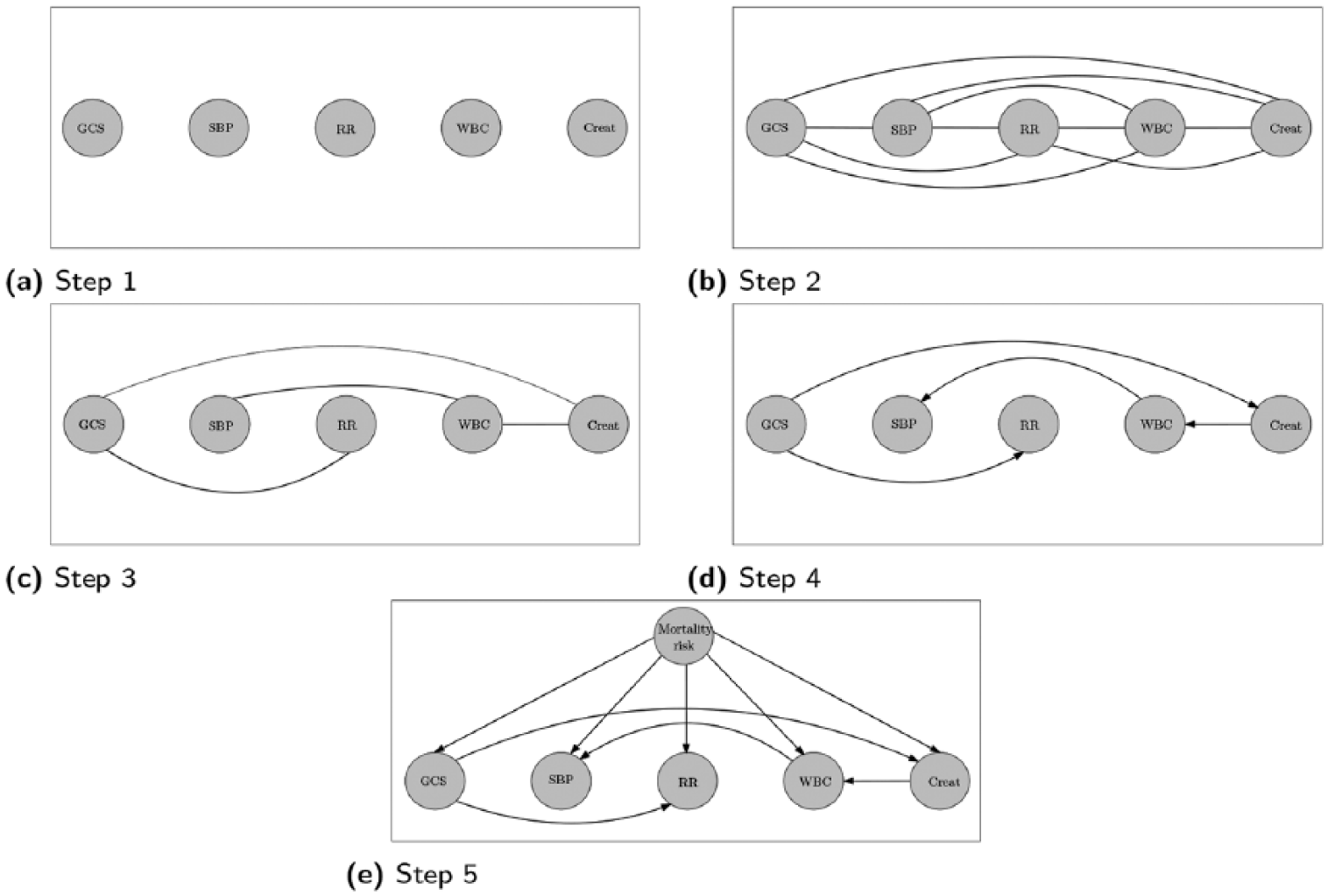
Structure learning of the TAN Bayesian network model.

After learning the TAN structure, the conditional probabilities are calculated using equation (3)

P (X_{i} | X_{p a (i)}) = \frac{P (X_{i}, X_{p a (i)})}{P (X_{p a (i)})} \forall i \in {G C S, S B P, R R, W B C, C r e a t}

(3)

$X_{p a (i)}$ are the parents of $X_{i}$ . For example, in Figure 9, the parents of RR are GCS and mortality risk. Therefore

P (X_{R R} | X_{G C S}, Y) = \frac{P (X_{R R}, X_{G C S}, Y)}{P (X_{G C S}, Y)}

The estimated conditional probabilities were used for the inference. For our model, the inference can be derived using Bayes’ theorem as follows

\begin{array}{l} P (Y | X_{G C S}, X_{S B P}, X_{R R}, X_{W B C}, X_{C r e a t}) = \frac{1}{Z} P (X_{G C S} | Y) P (X_{S B P} | Y, X_{W B C}) P (X_{R R} | Y, X_{G C S}) \\ P (X_{W B C} | Y, X_{C r e a t}) P (X_{C r e a t} | Y, X_{G C S}) P (Y) \end{array}

(4)

$Z$ is a scaling factor and equal to $P (X_{G C S}, X_{S B P}, X_{R R}, X_{W B C}, X_{C r e a t})$ .

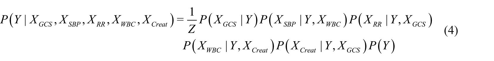
The inclusion of interactions among biomarkers differentiates our model from others. Most relationships discovered by TAN Bayesian network were supported by practitioner knowledge except the relationship between WBC and blood pressure. Based on expert’s opinions, the GCS is most likely to relate with RR and creatinine, and creatinine possibly affects WBC; but the relationship between WBC and blood pressure is not so apparent. Our results show eliminating the arc between WBC and blood pressure will marginally lower the overall performance of the model. Furthermore, we inspected the correlation coefficient between WBC and blood pressure and observed statistically significant negative correlation ( $ρ$ = –0.12). The negative correlation coefficient implies that as WBC increases, blood pressure decreases and vice versa. The magnitude of correlation coefficient represents the strength of association. Our findings suggest there might exist a relationship between WBC and blood pressure, and it warrants further investigation.

Results and discussion

In this section, we compare the performance of the proposed model with SIRS, qSOFA, MEWS, and SOFA. It is worth noting that MEWS and SOFA are not designed to predict mortality. MEWS is used to detect criticality of ill patients, and SOFA is used to understand the health of body organs. However, these criteria are commonly used in medical settings and provide a good benchmark to evaluate the performance of a model.³⁸

The metrics to evaluate the performance of a classifier are AUROC, sensitivity, specificity, and geometric mean (G-mean). The AUROC is most commonly used in medical literature to evaluate the diagnostic capability of a classifier as its discriminative threshold is varied. The AUROC of 1 corresponds to an ideal model, while 0.5 corresponds to the worst. Sensitivity is the true positive rate, and specificity is the true negative rate. G-mean is the geometric mean of sensitivity and specificity.

G - m e a n = \sqrt{s e n s i t i v i t y \times s p e c i f i c i t y}

(5)

G-mean is often used to inspect the balance between sensitivity and specificity.¹⁵

Our model estimates the risk of mortality. The estimated probabilities were translated into categorical outcome by using a cut-off point. This cut-off point governs the trade-off between sensitivity and specificity, therefore, the selection of cut-off point was given special attention. Instead of using default decision threshold (0.5), we explored previous studies to understand the best approaches to find the optimal cut-off point without considering the misclassification cost and prevalence. There exist two popular methods to find the optimal cut-off point: (1) point in receiver operating characteristic curve closer to (0, 1); first index represents false positive rate and second represents true positive rate, and (2) Youden index.^39,40 Youden index determines the cut-off at which (sensitivity + specificity: –1) is maximum. Perkins and Schisterman³⁹ compared these two methods and identified advantages and disadvantages of selecting one over the other. The ideal model passes through the point (0, 1). Therefore, any point in receiver operating characteristic curve closer to (0, 1) is visually more meaningful.³⁹ Hence, cut-off point corresponding to the point closer to (0, 1) was considered as an optimal cut-off point and was used to estimate sensitivity and specificity.

The model validation was performed using fivefold cross-validation. Figure 10 illustrates the validation procedure. We divided the data into five equal folds. One fold was used for the validation and the remaining were used to train the model. This procedure was carried out iteratively to consider each fold for validation. The final performance measures (AUROC, sensitivity, specificity and G-mean) were estimated by taking the average of performance measures obtained from five mutually exclusive data folds.

Figure 10.

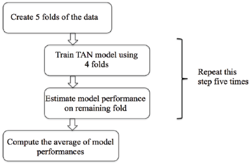
Model validation approach.

We compared the AUROC of the proposed model against the alternate models (SIRS, qSOFA, MEWS, and SOFA) over different time instances prior to discharge. Figure 11 illustrates the AUROC of our model and competing models preceding the discharge time. The result indicates that our model performed better than competing models over all time instances before the discharge. The percentage differences in AUROC between our model and the alternate models (SIRS, qSOFA, MEWS, and SOFA) ranged from 30%–50%, 22%–32%, 8%–11%, 3%–5%, respectively. This longitudinal analysis presents results in favor of the robustness of our model.

Figure 11.

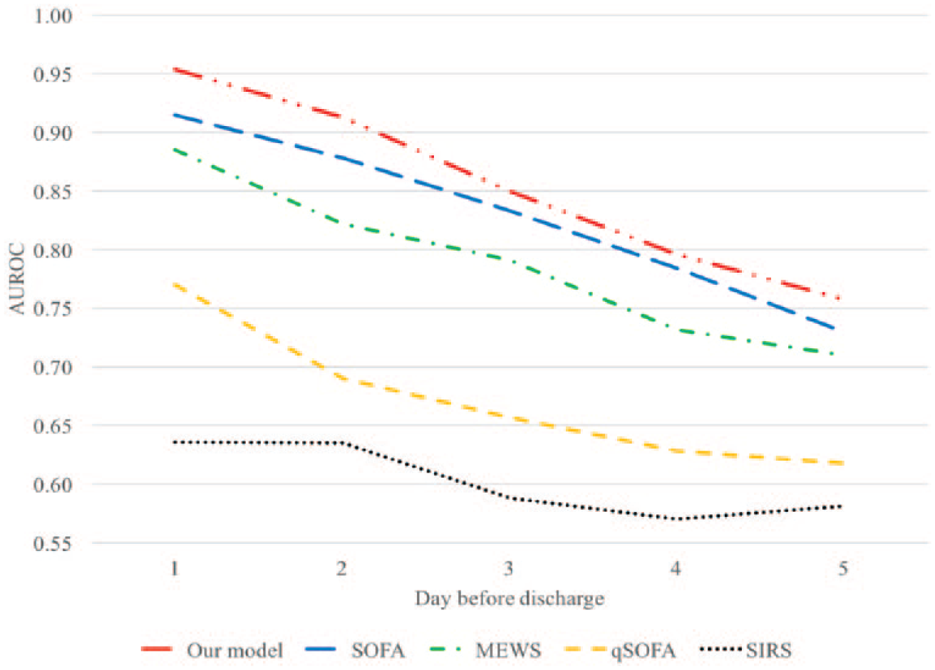
AUROC over the different time before the discharge.

We also compared the time-average performance of our model to alternate models (SIRS, qSOFA, MEWS, and SOFA). The sensitivity, specificity, G-mean, and AUROC of our model and competing models are shown in Figure 12. With AUROC of 0.84, our model outperformed other criteria (SIRS = 0.59, qSOFA = 0.65, MEWS = 0.75, SOFA = 0.80). In addition, our model provides the best balance between sensitivity and specificity, and this can be seen evidently using G-mean. The G-mean of our model (0.75) is greater than SIRS (0.55), qSOFA (0.58), MEWS (0.70), and SOFA (0.73).

Figure 12.

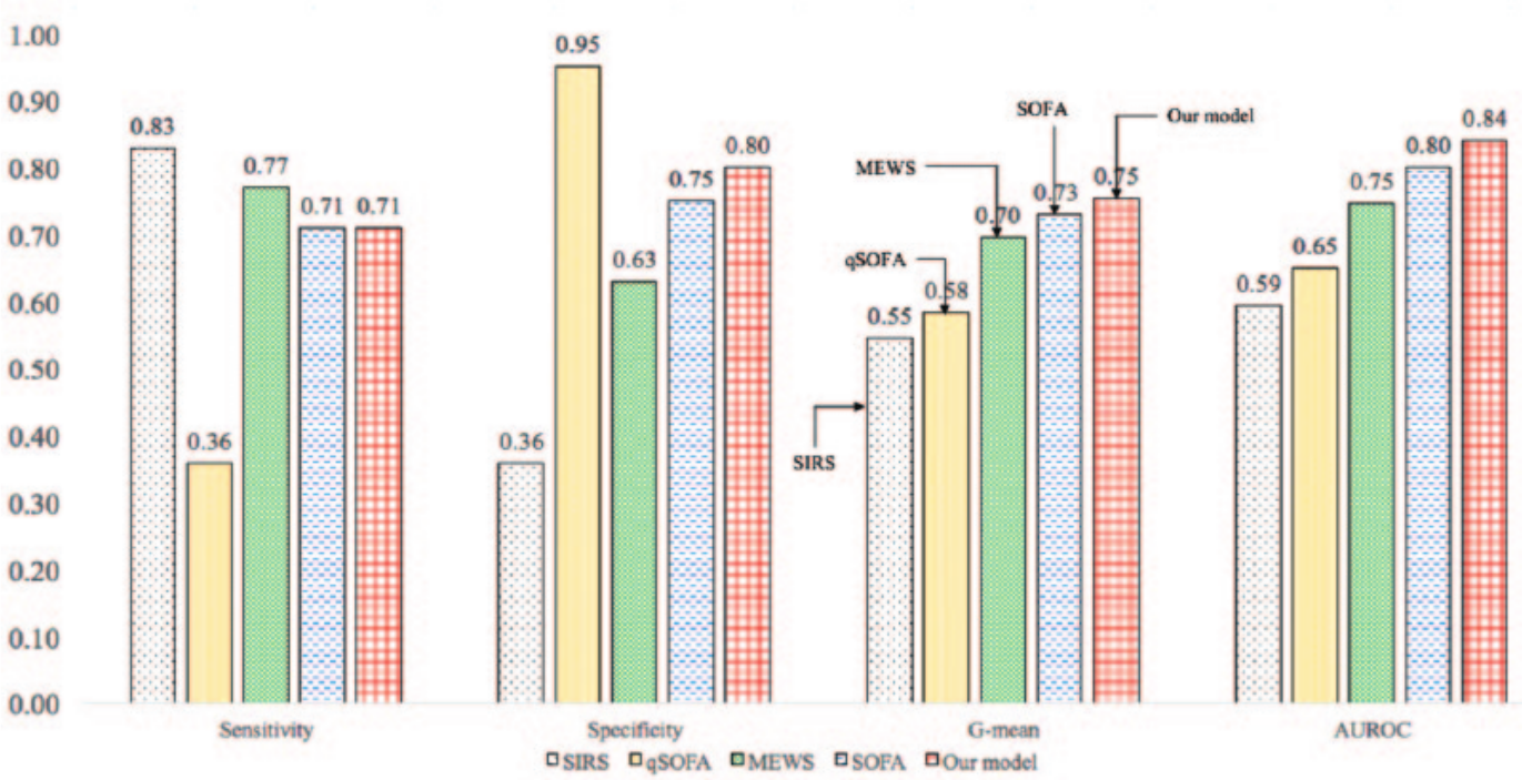
Comparison of performance of different diagnostic criteria.

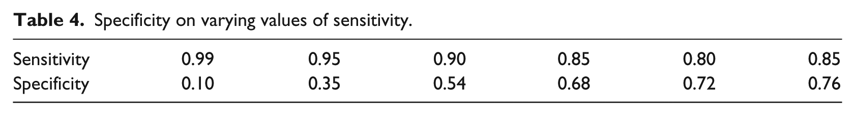
Many clinical applications of a model necessitate high sensitivity. Therefore, for the same AUROC (0.84), Table 4 reports specificity on varying values of sensitivity. The results show that at very high sensitivity (0.99), the model loses the specificity significantly. Depending on the requirement on sensitivity, we can increase the specificity.

Table 4.

Specificity on varying values of sensitivity.

Sensitivity	0.99	0.95	0.90	0.85	0.80	0.85
Specificity	0.10	0.35	0.54	0.68	0.72	0.76

The primary reason for the better performance using TAN Bayesian network is the presence of correlations among biomarkers. TAN considers correlations, while other modeling techniques treat all variables as independent. TAN Bayesian network usually performs better when variables are correlated.¹⁷ The physiological variables more often than not show correlation among biomarkers. For example, in our EHR data, the correlation between WBC and blood pressure is –0.12. Therefore, the performance gain of our model could be attributed to the existence of correlation among biomarkers.

Table 5 summarizes selected biomarkers and the performance characteristics of each model. Although our model uses more variables than SIRS and qSOFA, it performs significantly better than these models. SOFA score requires the knowledge of four laboratory results. Our model with only two laboratory results performs marginally better than SOFA. The use of fewer laboratory results enables practitioners to predict the risk of sepsis easily and quickly. The performance gain of our model using TAN Bayesian network is attributed to the presence of correlation between biomarkers in EHR data.

Table 5.

Biomarkers and the performance characteristics of different sepsis prognostic models.

	SIRS	qSOFA	MEWS	SOFA	Our model
Biomarkers
Systolic blood pressure		✓	✓	✓	✓
Glasgow coma scale		✓	✓	✓	✓
Respiratory rate	✓	✓	✓		✓
White blood cell	✓				✓
Creatinine					✓
$P a O_{2} / F i O_{2}$				✓	✓
Platelet count				✓
Mean arterial pressure				✓
Bilirubin				✓
Blood pressure support				✓
Body temperature	✓		✓
Hourly urine			✓
Heart rate	✓		✓
Number of biomarkers	4	3	6	8	5
Performance
AUROC	0.59	0.65	0.75	0.80	0.84
G-mean	0.55	0.58	0.70	0.73	0.75
Sensitivity	0.83	0.36	0.77	0.71	0.71
Specificity	0.36	0.95	0.63	0.75	0.80

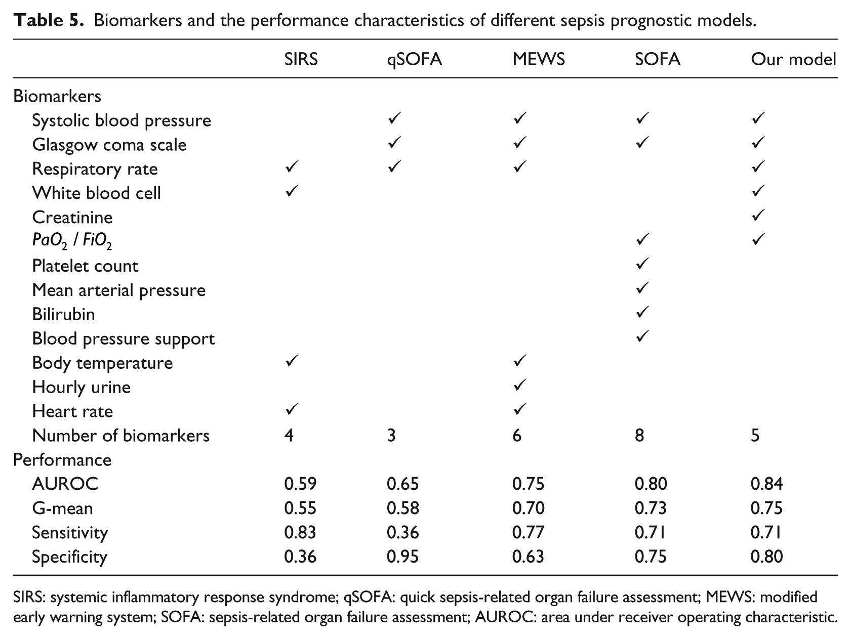
SIRS: systemic inflammatory response syndrome; qSOFA: quick sepsis-related organ failure assessment; MEWS: modified early warning system; SOFA: sepsis-related organ failure assessment; AUROC: area under receiver operating characteristic.

Conclusion

In this article, we developed a predictive model using TAN Bayesian network that inherently captures the important interactions among biomarkers and compared the performance of our model with SIRS, qSOFA, MEWS, and SOFA. The proposed model was trained with the population selected using the new sepsis definitions. The model development process includes the following main steps: data extraction, data preprocessing, learning of TAN Bayesian network, and model evaluation. The variable selection identifies biomarkers meaningful to predict sepsis. Out of a set of 13 variables, five variables were selected (SBP, GCS, RR, WBC count, and creatinine) to develop the TAN model.

The structure of the TAN network facilitates visual interpretation of the interactions among biomarkers. The model identified relations that were in align with practitioners’ knowledge. The comparative analysis showed that our model outperformed alternate models. The results underline the robustness of our model by comparing the AUROC of various models over different time instances prior to discharge. The proposed model eliminates the existing problem of unbalanced sensitivity (SIRS = 0.83, qSOFA = 0.36) and specificity (SIRS = 0.36, qSOFA = 0.95) and delivers balanced sensitivity (0.71) and specificity (0.80). The key characteristic of our model is that it outperformed MEWS and SOFA and uses fewer variables than them. The use of fewer lab results enables quick prognosis of sepsis. In comparison with SIRS, qSOFA, MEWS, and SOFA, our model provides the best alternative and can easily be integrated in EHR environment and autonomously identify the patient at high risk of sepsis.

The limitation of this study is that the data come only from hospitals using Cerners EHR system. So, there could be potential sources of bias in the data. Although we included data from hospitals located in all four U.S. census regions, we cannot generalize the results to all U.S. hospitals as there could be distinct differences between hospitals using the Cerner system and other hospitals. The possible reason of difference is that the Cerner’s EHR is mainly used in big hospitals because it is expensive to implement. We did not consider the effect of intervention by assuming that each patient was subjected to a similar intervention.

Footnotes

Authors’ Note

This work was conducted with data from the Cerner Corporation’s Health Facts database of electronic medical records provided by the Oklahoma State University Center for Health Systems Innovation (CHSI). Any opinions, findings, and conclusions or recommendations expressed in this material are those of the authors and do not necessarily reflect the views of the Cerner Corporation.

Declaration of conflicting interests

The author(s) declared no potential conflicts of interest with respect to the research, authorship, and/or publication of this article.

Funding

The author(s) received no financial support for the research, authorship, and/or publication of this article.

ORCID iD

Akash Gupta

References

Singer

Deutschman

Seymour

, et al. The third international consensus definitions for sepsis and septic shock (sepsis-3). JAMA 2016; 315(8): 801–810.

Freund

Lemachatti

Krastinova

, et al. Prognostic accuracy of Sepsis-3 criteria for in-hospital mortality among patients with suspected infection presenting to the emergency department. JAMA 2017; 317(3): 301–308.

Fleischmann

Scherag

Adhikari

, et al. Assessment of global incidence and mortality of hospital-treated sepsis. Current estimates and limitations. Am J Respir Crit Care Med 2016; 193(3): 259–272.

Torio

Andrews

. National inpatient hospital costs: the most expensive conditions by payer, 2011. Statistical brief #160, February 2006. Rockville, MD: Agency for Healthcare Research and Quality.

Seymour

Liu

Iwashyna

, et al. Assessment of clinical criteria for sepsis: for the third international consensus definitions for sepsis and septic shock (Sepsis-3). JAMA 2016; 315(8): 762–774.

Kaukonen

Bailey

Pilcher

, et al. Systemic inflammatory response syndrome criteria in defining severe sepsis. N Engl J Med 2015; 372(17): 1629–1638.

Ribas

Vellido

Ruiz-Rodríguez

, et al. Severe sepsis mortality prediction with logistic regression over latent factors. Expert Syst Appl 2012; 39(2): 1937–1943.

Gupta

Liu

Shepherd

, et al. Using statistical and machine learning methods to evaluate the prognostic accuracy of SIRS and qSOFA. Healthc Inform Res 2018; 24(2): 139–147.

Ghanem-Zoubi

Vardi

Laor

, et al. Assessment of disease-severity scoring systems for patients with sepsis in general internal medicine departments. Crit Care 2011; 15(2): R95.

10.

Grissom

Brown

Kuttler

, et al. A modified sequential organ failure assessment score for critical care triage. Disaster Med Public Health Prep 2010; 4(4): 277–284.

11.

Dorsett

Kroll

Smith

, et al. qSOFA has poor sensitivity for prehospital identification of severe sepsis and septic shock. Prehosp Emerg Care 2017; 21(4): 489–497.

12.

Gultepe

Green

Nguyen

, et al. From vital signs to clinical outcomes for patients with sepsis: a machine learning basis for a clinical decision support system. J Am Med Inform Assoc 2014; 21: 315–325.

13.

Peelen

de Keizer

Jonge

, et al. Using hierarchical dynamic Bayesian networks to investigate dynamics of organ failure in patients in the intensive care unit. J Biomed Inform 2010; 43(2): 273–286.

14.

Kaewprag

Newton

Vermillion

, et al. Predictive models for pressure ulcers from intensive care unit electronic health records using Bayesian networks. BMC Med Inform Decis Mak 2017; 17(Suppl. 2): 65.

15.

Topuz

Uner

Oztekin

, et al. Predicting pediatric clinic no-shows: a decision analytic framework using elastic net and bayesian belief network. Ann Oper Res 2018; 263: 479–499.

16.

Friedman

Geiger

Goldszmidt

. Bayesian network classifiers. Mach Learn 1997; 29(2–3): 131–163.

17.

Padmanaban

. Comparative analysis of naive Bayes and tree augmented naive Bayes models. MSc Thesis, 2014, https://pdfs.semanticscholar.org/e900/94e6d44ebd61193e0411c82515a66ef8eec2.pdf

18.

Le Gall

Klar

Lemeshow

, et al. The logistic organ dysfunction system: a new way to assess organ dysfunction in the intensive care unit. JAMA 1996; 276(10): 802–810.

19.

Bone

Balk

Cerra

, et al. Definitions for sepsis and organ failure and guidelines for the use of innovative therapies in sepsis. Chest 1992; 101(6): 1644–1655.

20.

Subbe

Kruger

Rutherford

, et al. Validation of a modified early warning score in medical admissions. QJM 2001; 94(10): 521–526.

21.

Vincent

Moreno

Takala

, et al. The SOFA (Sepsis-related organ failure assessment) score to describe organ dysfunction/failure. On behalf of the Working Group on Sepsis-Related Problems of the European Society of Intensive Care Medicine. Intensive Care Med 1996; 22(7): 707–710.

22.

Mathe

Ledeczi

Nadas

, et al. A model-integrated, guideline-driven, clinical decision-support system. IEEE Software 2009; 26(4): 54–61.

23.

Brandt

Gartner

Moncure

, et al. Identifying severe sepsis via electronic surveillance. Am J Med Qual 2015; 30(6): 559–565.

24.

Amland

Hahn-Cover

. Clinical decision support for early recognition of sepsis. Am J Med Qual 2016; 31(2): 103–110.

25.

Henry

Hager

Pronovost

, et al. A targeted real-time early warning score (trewscore) for septic shock. Sci Transl Med 2015; 7(299): 299ra122.

26.

Mani

Ozdas

Aliferis

, et al. Medical decision support using machine learning for early detection of late-onset neonatal sepsis. J Am Med Inform Assoc 2014; 21(2): 326–336.

27.

Nemzek

Hodges

. Bayesian network analysis of multi-compartmentalized immune responses in a murine model of sepsis and direct lung injury. BMC Res Notes 2015; 8(1): 516.

28.

Sandri

Berchialla

Baldi

, et al. Dynamic Bayesian networks to predict sequences of organ failures in patients admitted to ICU. J Biomed Inform 2014; 48: 106–113.

29.

DeShazo

Hoffman

. A comparison of a multistate inpatient EHR database to the HCUP nationwide inpatient sample. BMC Health Serv Res 2015; 15(1): 384.

30.

Hartemink

. Principled computational methods for the validation discovery of genetic regulatory networks. PhD Thesis, Massachusetts Institute of Technology, Cambridge, MA, 2001.

31.

Capan

Hoover

Ivy

, et al. Not all organ dysfunctions are created equal—prevalence and mortality in sepsis. J Crit Care 2018; 48: 257–262.

32.

Zou

Hastie

. Regularization and variable selection via the elastic net. J R Statist Soc 2005; 67(2): 301–320.

33.

Therneau

Atkinson

. An introduction to recursive partitioning using the RPART routines. Rochester, NY: Mayo Foundation, 1997.

34.

Raileanu

Stoffel

. Theoretical comparison between the Gini index and information gain criteria. Ann Math Artif Intel 2004; 41(1): 77–93.

35.

Sakia

. The Box-Cox transformation technique: a review. Statistician 1992; 41: 169–178.

36.

Koller

Friedman

. Probabilistic graphical models: principles and techniques. Cambridge, MA: MIT Press, 2009.

37.

Chow

Liu

. Approximating discrete probability distributions with dependence trees. IEEE T Inform Theory 1968; 14(3): 462–467.

38.

Desautels

Calvert