Sage Journals: Discover world-class research

Abstract

The number and timing of unplanned admissions to inpatient teaching services vary. Recent changes to resident duty hours make it essential to maximize learning experiences and balance workload on these services. Queueing theory provides a mechanism for understanding and planning for the variations in admissions and daily census. Daily admissions, length of stay, and daily census were modeled for a teaching inpatient family medicine service over 46 months using an M/G/∞ queueing model. Q–Q plots and a Kolmogorov–Smirnov test were used to check the fit of actual data to the model. Admissions and daily census followed a Poisson distribution (λ = 3.28 and λ = 8.28, respectively), while length-of-stay followed a lognormal distribution (µ = 0.49, σ2 = 0.83). The M/G/∞ queueing model proved useful for predicting overflow admission frequency, defining expected resident workload in terms of patient-days, and determining hospital unit size requirements.

Keywords

inpatients internship and residency patient admission queueing theory systems theory

Introduction

The number of unplanned admissions to a teaching family medicine inpatient hospital service varies from one day to another. Proposed Family Medicine Residency Review Committee (RRC) rules will require a “minimum of 600 hours or six blocks/months and 750 patient encounters dedicated to the care of hospitalized adult patients” for family medicine residents.¹ Recent changes in resident duty hours² make it vital to maximize learning experiences and balance workload by staffing rotations appropriately in order to meet these requirements.^3–7 Additionally, multidisciplinary rounds on a hospital unit have been shown to increase teamwork and decrease adverse events.^8–10 Overflowing patients to various other hospital units may be detrimental to quality patient care.

Thus, in order to care for patients in an optimal manner and assure adequate inpatient learning experiences for residents, it is important to understand and plan for the daily variation in admissions. When considering how the inpatient family medicine service operates, three key management scenarios arise:

For patient safety and teaching purposes, we would like to limit junior residents to six admissions per day. How often would a backup system need to be activated to meet patient demand?

What is the average workload residents currently receive? Can they achieve the required 750 patient encounters while devoting 6 months to the family medicine service during their residency?

We would like to keep patients on our own unit 95 percent of the time to ensure good teamwork. How many beds should be available to accomplish this?

Queueing theory is the formal mathematical study of systems that provide service for randomly arising demands.¹¹ Although originally developed for use in telecommunications, queueing theory has been used in many fields including computing, factory design, and traffic engineering.^11,12 In health care, queueing theory has been studied to evaluate emergency department flow,¹³ optimize intensive care unit (ICU) admissions,^14–16 determine scheduled admission quotas,¹⁷ improve patient registry services,¹⁸ and examine placement in skilled care facilities.¹⁹

A basic queueing model is characterized by the independent arrival of patients and the service or care of those patients by healthcare providers in an inpatient setting. By knowing two generally available characteristics of any inpatient service with unplanned admissions, the mean admission rate and mean length of stay, a queueing model can predict the parameters necessary to effectively answer the scenarios posed above.

Methods

Setting

The family medicine inpatient service shares a 31-bed hospital unit with neurology at St Mary’s Hospital in Rochester, Minnesota (a 1265-bed facility). On average, one-third of the occupied beds on the unit are family medicine patients. The service accepts community patients who have a primary care physician at the Mayo Clinic Department of Family Medicine and require inpatient medical treatment. No monitored beds or ICU-level care is available on the service. The service currently admits approximately 1200 patients per year. Patients are frequently admitted thru the hospital’s emergency department, but admissions also occur directly from outpatient clinics or hospital service transfers such as a patient no longer needing ICU-level care. Since there is no service size or admission cap, patients sometimes overflow to various other locations in the hospital when a bed on the primary unit is not immediately available.

The service is supervised by a staff family medicine physician acting as a teaching hospitalist for 1 week at a time. Three PGY2 or PGY3 level residents cover the service, admitting new patients every third day. A PGY1 resident is sometimes present for 12-h shifts and is directly supervised by the on-call resident.

Data

The number of daily admissions to the family medicine service and the 7 a.m. census was collected from 21 June 2008 thru 3 May 2012, in a de-identified manner from a patient registry maintained by the service. Length of stay information was available in the registry and collected from 1 January 2012 thru 3 May 2012. Because no individual patient identifying information was collected, the Institutional Review Board deemed the study exempt.

Data were stored in a Postgres version 9.1.3 relational database for subsequent retrieval and analysis. Analysis was performed using R version 2.15.0 running on Mac OS X 10.7.3.

Queueing model

A basic queueing model in medicine is characterized by the arrival of patients and the service or care of those patients by healthcare providers. Classically, the arrival process is modeled by a Poisson distribution which assumes an average rate of arrival with each particular arrival independent of others. Each individual patient within the department of family medicine has a very small probability p of requiring hospitalization within a given day. We can regard each patient as an independent Bernoulli trial Bern(p) with hospitalization defined as success. The sum of n Bernoulli trials results in a Binomial distribution B(n, p). If n is large and p is very small, B(n, p) may be approximated by the Poisson distribution with λ = np^12,20

P o i s_{k} (λ) = \frac{λ^{k}}{k!} e^{- λ} for k \geq 0

(1)

The department of family medicine cares for over 100,000 community patients and typically fewer than 20 of these are hospitalized on the family medicine service on any given day, so our assumptions about daily admissions appear reasonable.

In queueing theory, the service time is classically modeled with an exponential distribution.¹² The mathematical properties of this distribution allow the derivation of several closed-form solutions to common performance measures.^11,12 In our case, the service time is equivalent to the length of stay for each patient in the hospital. Due to the complexities of medical care for individual patients, no theoretical model exists to explain the length of stay distribution.²¹ However, exponential and mixed exponential distributions have been fitted to actual length of stay data for psychiatric patients²² and private hospital patients,²³ while lognormal distributions have been fitted to hospital stays grouped by diagnosis-related groups (DRGs).²⁴ We chose to examine both of these distributions.

In our case, we assume patients are treated in parallel by the on-call resident who has sufficient service capacity and patients will not leave the queue to seek care elsewhere. There is no waiting time, and therefore, the sojourn time is equal to the service time. Thus, this represents an M/M/∞ queueing model using Kendall’s notation.¹² The census or expected number of patients in the system E(L) is equal to the mean amount of work that arrives per unit time, ρ¹². By Little’s Law, this is equivalent to the arrival rate multiplied by the expected service time E(B), irrespective of the service time distribution

E (L) = λ E (B) = ρ

(2)

It can also be shown that the probability p_n of n patients in the system is a Poisson distribution with mean ρ¹²

p_{n} = \frac{p^{n}}{n!} e^{- ρ} = P o i s (λ E (B))

(3)

Thus, we are able to express the distribution of the daily hospital census as a function of the admission rate and the mean length of stay.

Goodness of fit

There are numerous ways of comparing observed data to expected distributions to assess goodness of fit. For each of our observed distributions (admissions, length of stay, and census), we calculated descriptive statistics such as mean and variance and compared these to the expected theoretic values. For instance, the mean is equal to the variance in a Poisson distribution. A histogram of the observed data was generated and the expected distribution was overlaid to provide a graphical comparison. Another graphical technique is the Q–Q plot which compares two probability distributions by plotting their quantiles against each other. If the observed data are similar to the expected distribution, the data points lie on the line y = x.

The classical numeric test for goodness of fit in discrete data is the Pearson chi-square test. It groups the probability mass function into bins and compares the observed counts to the expected counts within each bin. Bin counts less than five are problematic for the chi-square assumptions and by convention are usually combined with adjacent bins to produce counts over five. Bins are given equal weight and order is not considered. While this is useful for nominal variables, information is lost when numeric variables are binned.²⁵ Additionally, the chi-square test becomes more powerful as sample size increases. Thus, small and scientifically unimportant departures from an expected distribution, particularly in the tails, may be detected with large sample sizes.²⁶

The Kolmogorov–Smirnov test is another hypothesis test that numerically assesses goodness of fit. It measures the distance the observed data are from the expected cumulative probability distribution (CDF) and was originally designed to be applied to continuous distributions. However, it has been adapted to discrete distributions with p-values computed by Monte Carlo simulation.²⁷ The Kolmogorov–Smirnov test utilizes each observation without grouping and weights them equally.

Our null hypothesis in each case is the observed data follow the expected theoretic distribution. To evaluate these hypotheses, we chose to perform the Kolmogorov–Smirnov test with p < 0.05, indicating that the null hypothesis should be rejected.

Results

Arrival distribution

Figure 1 shows a histogram of the daily admission totals to the family medicine service over 1404 days. The mean number of daily admissions was 3.28 with a variance of 3.62. As expected, the mean and variance are close and a Poisson distribution of admissions is likely a good approximation. A theoretic Poisson distribution with λ = 3.28 admissions/day is plotted on the histogram and demonstrates good correlation visually. The Q–Q plot of predicted versus actual admissions seen in Figure 1 shows great similarity graphically. A Kolmogorov–Smirnov test was performed with a null hypothesis that the observed data follow a Poisson distribution with λ = 3.28. In this case, p = 0.6508, and we cannot reject the null hypothesis that the actual and predicted distributions are similar. Thus, we have good graphical and statistical evidence that daily admissions to this family medicine service follow a Poisson distribution with λ = 3.28.

Figure 1.

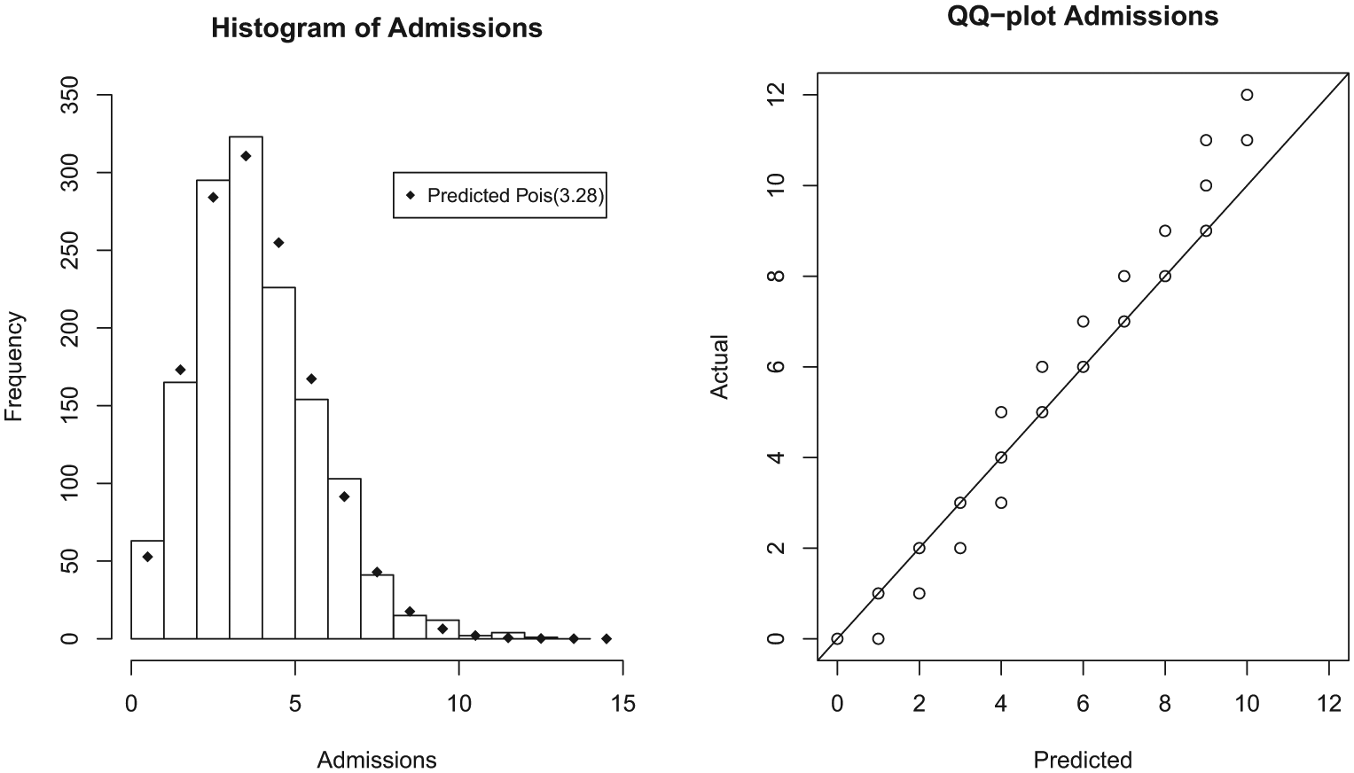
Admissions.

Service time distribution

Figure 2 shows a histogram of the lengths of stays, measured in days, for 700 patients admitted to the family medicine service. The mean length of stay was 2.27 days with a variance of 4.04. A theoretic exponential distribution with λ = 1/2.27 = 0.44 was fitted to the data and is plotted as a solid line. Looking at the graph, the theoretic exponential distribution seems to overestimate the probability of extremely short stays. The Q–Q plot shows some correlation, but deviation is evident with underestimation of actual tail probabilities. A Kolmogorov–Smirnov test showed p < 0.0001, leading us to reject the null hypothesis that the observed length of stay is exponentially distributed.

Figure 2.

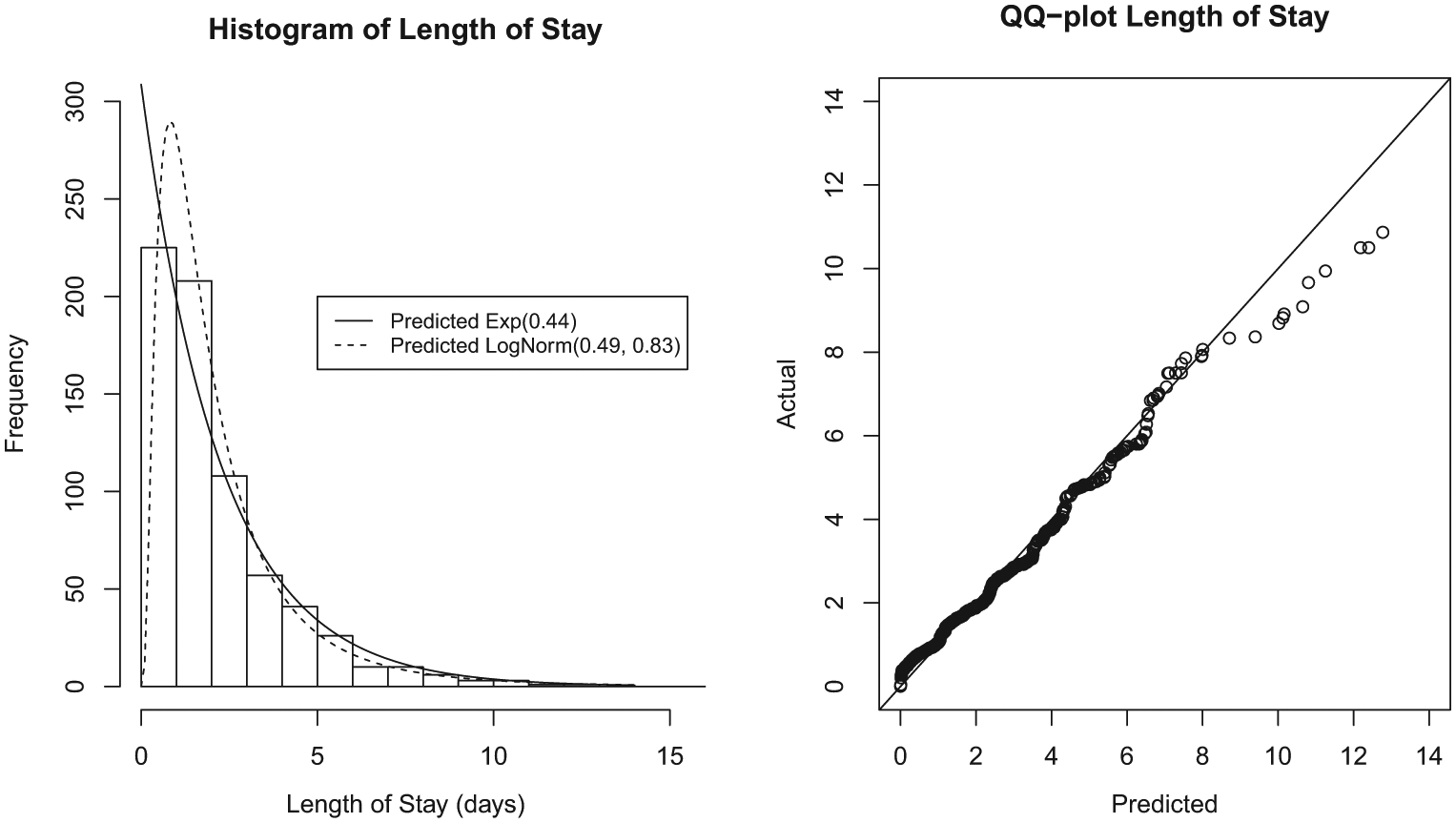
Length of stay.

Subsequently, a lognormal distribution with µ = 0.49 and σ² = 0.83 was fitted to the observed data after inspecting the histogram. A Kolmogorov–Smirnov test shows p = 0.3128, and thus, we retain the null hypothesis that the observed data are similar to a theoretical lognormal distribution.

Census distribution

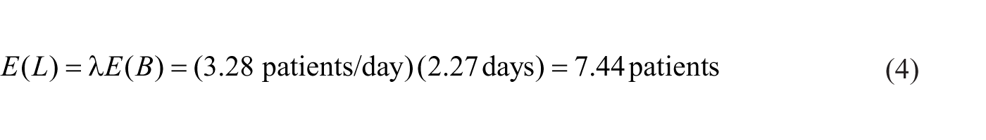
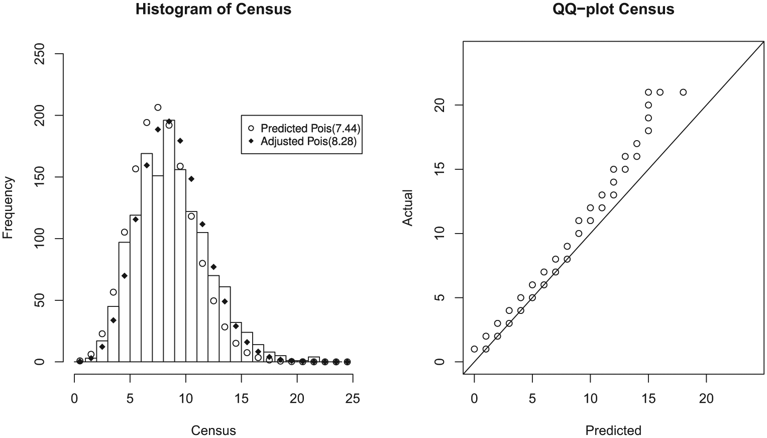
Figure 3 shows a histogram of the daily 7 a.m. census for the family medicine hospital service over 1400 days. The mean observed 7 a.m. census is 8.28 patients with a variance of 10.56. As was shown in equation (2), the expected census is equivalent to the amount of work that arrives per day which is the admission rate multiplied by the expected length of stay

E (L) = λ E (B) = (3.28 patients/day) (2.27 days) = 7.44 patients

(4)

Figure 3.

Census.

Thus, our expected census is 7.44 patients, and a Poisson distribution with mean 7.44 is plotted on the histogram for comparison. While the histogram appears to approximate a Poisson distribution, the expected values appear shifted slightly lower than the observed values. This is also easily seen on the Q–Q plot which lies roughly parallel to the unity line, but is shifted toward the higher observed values. A Kolmogorov–Smirnov test has p < 0.0001 leading us to reject the null hypothesis and conclude the actual and predicted distributions are somehow different.

Two possibilities exist, either the observed distribution has a different mean than predicted but remains a Poisson distribution, or it is not a Poisson distribution. We plotted a Poisson distribution with mean 8.28 on the histogram in Figure 3 (see the “Discussion” section). The Q–Q plot lies approximately parallel to the y = x line suggesting the distribution is similar to Poisson with a shifted mean. With a new null hypothesis that the observed distribution follows a Poisson distribution with mean 8.28, we performed a Kolmogorov–Smirnov test. In this case, p = 0.2487, and we cannot reject this null hypothesis. However, the variance is greater than the mean, suggesting overdispersion of a Poisson distribution, a common finding in observed count data.^28,29

Discussion

Queueing theory classically models the service time as an exponential distribution, making the mathematics easier. However, in the case of the family medicine service, the service time or length of stay did not fit a simplistic exponential distribution. Instead, the length of stay appears to be a lognormal distribution. This makes intuitive sense as the exponential distribution predicts a large probability of a zero length hospital stay, while the lognormal distribution accurately predicts a zero probability of a zero length hospital stay (see Figure 2). The logarithms of many biologic parameters are normally distributed giving rise to the lognormal distribution.^30,31 Additionally, a lognormal distribution has previously been observed for lengths of stay in patients grouped by DRGs and in a large study at an Israeli hospital.^24,32 This complicates the queueing model and changes it to an M/G/∞ model in Kendall’s notation. However, for such models, it can be shown that equations (2) and (3) still hold.¹²

Thus, the expected census E(L) remains equivalent to the expected admission rate λ multiplied by the expected length of stay E(B). Additionally, the census should be Poisson distributed. However, the queueing model predicts an expected census of 7.44 patients versus the observed 7 a.m. census of 8.28. One possible explanation for this difference is the fact that the 7 a.m. measurement time likely reflects a higher census than later in the day as most discharges do not happen until after morning rounds. The queueing model is predicting the census for the entire 24-h period, which is not necessarily the same as predicting the census at a particular time of day.

Scenario A—backup frequency

We have shown that admissions to the family medicine inpatient service follow a Poisson-distributed arrival process, thus explaining variability in the number of daily admissions. As stated in Scenario A, we are targeting a maximum of six admissions per day per resident. Since admissions follow a Poisson distribution, by knowing only the mean number of admissions per day, the probability of having seven or more admissions can be determined. The CDF for a Poisson distribution is given by the following equation

CDF (k) = e^{- λ} \sum_{i = 0}^{k} \frac{λ^{i}}{i!}

(5)

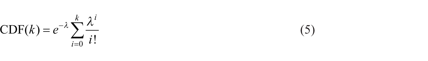
By substituting λ = 3.28 and k = 6 and subtracting the cumulative probability from 1, we get a probability of 0.0497 for seven or more admissions

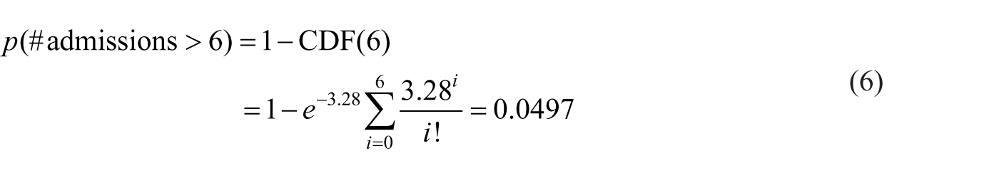
\begin{array}{l} p (# admissions > 6) = 1 - CDF (6) \\ = 1 - e^{- 3.28} \sum_{i = 0}^{6} \frac{{3.28}^{i}}{i!} = 0.0497 \end{array}

(6)

Thus, at the current admission rate, activating backup for a day with more than six admissions would be required about 5 percent of the time or 1 in 20 days.

Scenario B—resident workload

Resident workload has traditionally been measured by numbers of patients, either total census divided by the number of residents, or the number of admissions per resident.^4,6,7,33,34 Neither of these measurements account for differences in length of stay and the continuity care of patients throughout their hospitalization. We prefer a new quantity, the patient-day, as a measure of resident workload. This is analogous to the unit of work in physics which is defined as force multiplied by distance (ft-lbs or Newton-meters).³⁵ In our case, caring for a hospitalized patient (force) acts over the length of stay in days (distance) to produce physician workload. The proposed RRC rule changes are starting to recognize this and call for measuring resident experience in terms of “encounters”, which they define as caring for a hospitalized patient for 1 day.^1,36

From the queueing model, 7.44 patient-days of work are expected to arrive with a Poisson distribution each call day (equation (4)); 6 months of service represents 180 days with 60 call days per resident. If each resident follows the patients they admit throughout their hospitalization, they can expect (60) (7.44 patient-days) = 446 patient-days of workload. This is insufficient to meet the RRC standard of 750 “encounters” or patient-days. Thus, a redesign of the service is required in order to meet proposed RRC requirements.

Three redesign options for the family medicine service were evaluated as shown in Table 1. All options assumed the length of stay E(B) was unchanged. By convolution, the sum of the workload arriving over n independent call days for a resident is a Poisson distribution with mean nE(L). Thus, the cumulative distribution function (equation (5)) shows that a mean workload (nE(L)) of 797 patient-days is necessary to ensure 95 percent of residents will receive at least 750 patient-days of experience. In the first option, we calculated how long residents would need to be on service in order to meet RRC requirements if there were no changes in admission rate. The second option shows how much the admission rate would need to increase to meet RRC “encounter” requirements within the minimum required 6 months of service. The final option reflects anticipated growth in the department generating a modest increase in admission rate and a long enough resident rotation to meet RRC “encounter” requirements. These examples demonstrate how queueing theory can inform residency leadership about how various rotation options might meet RRC requirements.

Table 1.

Using queueing theory to redesign family medicine service (Scenario B).

Parameter	Current	Option 1^a	Option 2^b	Option 3^c
Admissions per day λ	3.28	3.28	5.85	4.28
Length of stay E(B)	2.27	2.27	2.27	2.27
Workload arriving per day E(L) = λE(B)	7.44	7.44	13.28	9.72
Months of call M	6	10.8	6	8.2
Call days (q3) D = M × 10	60	108	60	82
Total patient-days D × E(L)	446	797	797	797

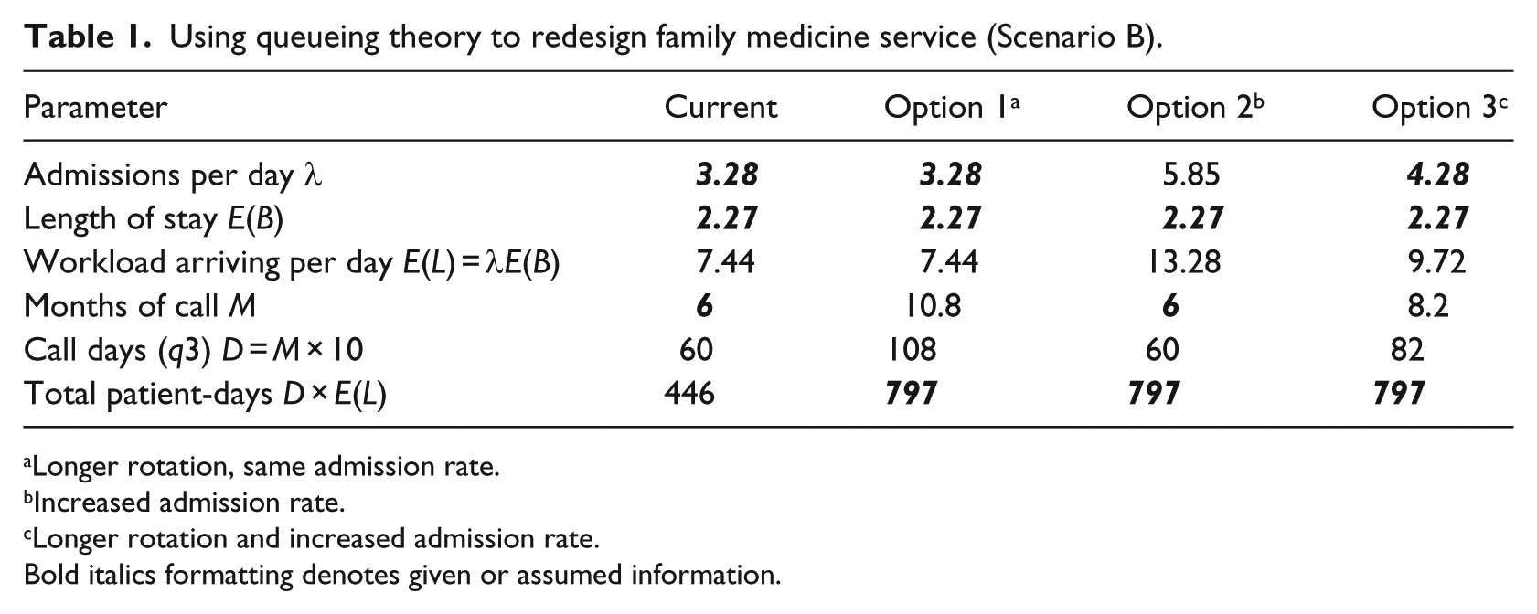
Longer rotation, same admission rate.

Increased admission rate.

Longer rotation and increased admission rate.

Bold italics formatting denotes given or assumed information.

Scenario C—unit size

To maintain quality, efficiency, and tight integration with nursing services, it is desirable to keep the majority of our hospitalized patients on one nursing unit. Knowing the mean census allows us to plan bed availability and unit size. We have targeted keeping patients on our own unit 95 percent of the time. Through equation (5) with λ = 7.44, we can iteratively solve for k such that the probability of exceeding k is less than 5 percent. In our case, this is k = 12, and we plan to have at least 12 beds available to our service on our nursing unit.

Limitations

An M/G/∞ queue implies unlimited service capacity, an obvious impossibility in real systems. However, the infinite server model serves as a useful approximation to the finite server case when demand is less than available capacity.³⁷ Physician service capacity and bed availability are not constraining factors under normal operating circumstances for the family medicine service at Saint Mary’s Hospital.

Length of stay information was not available within the registry prior to 1 January 2012. Due to the de-identified nature of the dataset, it was impossible to reconstruct length of stay information before that date. Thus, the length of stay data are based upon a shorter timeframe than the admission rate and census data. This could potentially affect the application of Little’s Law if the mean length of stay varies over the study period. However, prior work on this family medicine service shows that the length of stay found in this study was not different from the length of stay found in November 2008 thru October 2009, suggesting that the length of stay did not vary significantly during the study period.³⁸

The census data cannot be distinguished from a Poisson distribution using the Kolmogorov–Smirnov goodness-of-fit test. However, there is likely some overdispersion present with the variance greater than the mean. Since we are confident in the theoretical basis of the queueing model, the Pearson’s χ² statistic can be used to inflate the standard error of the quasi-Poisson distribution. In our case, this overdispersion would result in a 12.8 percent increase in the standard error estimate

Our data represent a pilot study of one inpatient teaching family medicine service. Although we predict the model is easily extended to other inpatient scenarios with unplanned admissions, further study is warranted to confirm general applicability.

Conclusion

To quote George Box, “all models are wrong, some are useful.” This work shows that the number of admissions per day and the daily census of a family medicine inpatient service are effectively modeled by Poisson-distributed random variables. The length of stay follows a lognormal distributed random variable. This leads to a M/G/∞ queueing system which provides a valuable model upon which to base administrative decisions regarding resident workload, staffing, and unit size.

Footnotes

Acknowledgements

We thank our clinical assistants Char Evans and Tiffany Matti who collected the daily admission data over the past 4 years that made this project possible.

Declaration of conflicting interests

The author(s) declared no potential conflicts of interest with respect to the research, authorship, and/or publication of this article.

Funding

The author(s) disclosed receipt of the following financial support for the research, authorship, and/or publication of this article: This work was supported by discretionary funding of the Department of Family Medicine, Mayo Clinic, Rochester, MN.

References

Draft of Proposed ACGME Program Requirements for Graduate Medical Education in Family Medicine, http://www.afmrd.org/files/PD%20Toolbox/RC-FM_Handout_2_Draft_Proposed_Program_Requirements_for_GME_in_FM.pdf (2012, accessed 17 June 2013).

The ACGME 2011 Duty Hour Standards: enhancing quality of care, supervision, and resident professional development, http://www.acgme-2010standards.org/pdf/monographs/jgme-monograph.pdf (2011, accessed 25 July 2012).

McCoy

Halvorsen

Loftus

. Effect of 16-hour duty periods on patient care and resident education. Mayo Clin Proc 2011; 86(3): 192–196.

Haney

Nicolaidis

Hunter

. Relationship between resident workload and self-perceived learning on inpatient medicine wards: a longitudinal study. BMC Med Educ 2006; 6: 35.

Fletcher

Underwood

3rd Davis

. Effects of work hour reduction on residents’ lives: a systematic review. JAMA 2005; 294(9): 1088–1100.

Coit

Katz

McMahon

. The effect of workload reduction on the quality of residents’ discharge summaries. J Gen Intern Med 2011; 26(1): 28–32.

Thanarajasingam

McDonald

Halvorsen

. Service census caps and unit-based admissions: resident workload, conference attendance, duty hour compliance, and patient safety. Mayo Clin Proc 2012; 87(4): 320–327.

O’Leary

Wayne

Haviley

. Improving teamwork: impact of structured interdisciplinary rounds on a medical teaching unit. J Gen Intern Med 2010; 25(8): 826–832.

O’Leary

Haviley

Slade

. Improving teamwork: impact of structured interdisciplinary rounds on a hospitalist unit. J Hosp Med 2011; 6(2): 88–93.

10.

O’Leary

Buck

Fligiel

. Structured interdisciplinary rounds in a medical teaching unit: improving patient safety. Arch Intern Med 2011; 171(7): 678–684.

11.

Gross

Shortle

Thompson

. Fundamentals of queueing theory. 4th ed. New York: Wiley, 2008.

12.

Adan

Resing

. Queueing theory. Eindhoven: Department of Mathematics and Computing Science, Eindhoven University of Technology, 2001.

13.

Green

Soares

Giglio

. Using queueing theory to increase the effectiveness of emergency department provider staffing. Acad Emerg Med 2006; 13(1): 61–68.

14.

Shmueli

Sprung

Kaplan

. Optimizing admissions to an intensive care unit. Health Care Manag Sci 2003; 6(3): 131–136.

15.

De Bruin

Van Rossum

Visser

. Modeling the emergency cardiac in-patient flow: an application of queuing theory. Health Care Manag Sci 2007; 10(2): 125–137.

16.

McManus

Long

Cooper

. Queuing theory accurately models the need for critical care resources. Anesthesiology 2004; 100(5): 1271–1276.

17.

Bekker

Koeleman

. Scheduling admissions and reducing variability in bed demand. Health Care Manag Sci 2011; 14(3): 237–249.

18.

Zai

Farr

Grant

. Queuing theory to guide the implementation of a heart failure inpatient registry program. J Am Med Inform Assoc 2009; 16(4): 516–523.

19.

Weiss

McClain

. Administrative days in acute care facilities: a queueing-analytic approach. Oper Res 1987; 35(1): 35–44.

20.

Agresti

. An introduction to categorical data analysis. New York: Wiley, 1996.

21.

Marshall

Vasilakis

El-Darzi

. Length of stay-based patient flow models: recent developments and future directions. Health Care Manag Sci 2005; 8(3): 213–220.

22.

Priest

Fineberg

Merson

. Length of stay of acute psychiatric inpatients: an exponential model. Acta Psychiatr Scand 1995; 92(4): 315–317.

23.

Harrison

. Implications of mixed exponential occupancy distributions and patient flow models for health care planning. Health Care Manag Sci 2001; 4(1): 37–45.

24.

Marazzi

Paccaud

Ruffieux

. Fitting the distributions of length of stay by parametric models. Med Care 1998; 36(6): 915–927.

25.

Royston

Altman

Sauerbrei

. Dichotomizing continuous predictors in multiple regression: a bad idea. Stat Med 2006; 25(1): 127–141.

26.

McLaren

Legler

Brittenham

. The generalized chi-square goodness-of-fit test. The Statistician 1994; 43(No. 2): 247–258.

27.

Arnold

Emerson

. Nonparametric goodness-of-fit tests for discrete null distributions. R Journal 2011; 3(2): 34–39.

28.

Rodriguez

. Models for count data with overdispersion. Princeton, NJ: Princeton University, 2013.

29.

Ver Hoef

Boveng

. Quasi-Poisson vs. negative binomial regression: how should we model overdispersed count data? Ecology 2007; 88(11): 2766–2772.

30.

Makuch

Freeman

Jr Johnson

. Justification for the lognormal distribution as a model for blood pressure. J Chronic Dis 1979; 32(3): 245–250.

31.

Abrahamyan

Beyene

Feng

. Response times follow lognormal or gamma distribution in arthritis patients. J Clin Epidemiol 2010; 63(12): 1363–1369.

32.

Armony

Israelit

Mandelbaum

. Patient flow in hospitals: a data-based queueing-science perspective. Stoch Syst 2011, http://mechroom.technion.ac.il/serveng/References/Patient%20flow%20main.pdf

33.

Dellit

Armas-Loughran

Bosl

. A method for assessing house staff workload as a function of length of stay. JAMA 2001; 286(9): 1023–1024.

34.

Fletcher

Reed

Arora

. Doing the dirty work: measuring and optimizing resident workload. J Gen Intern Med 2011; 26(1): 8–9.

35.

Ohanian

. Physics. 2nd ed. New York: W. W. Norton & Company, 1989.

36.

Martin

Meyer

. Family medicine review committee update. Paper presented at program directors workshop, Kansas City, MO, 12 June 2011.

37.

Whitt

. The infinite-server queueing model: the center of the many-server Queueing Universe (i.e., More Relevant Than It Might Seem), http://www.columbia.edu/~ww2040/8100S12/ISqueue021412.pdf (2012, accessed 18 June 2013).

38.

Garrison

Mansukhani

Bohn

. Predictors of thirty-day readmission among hospitalized family medicine patients. J Am Board Fam Med 2013; 26(1): 71–77.

39.

Box

GEP

Draper

. Empirical model building and response surfaces. New York: John Wiley & Sons, 1987.

Using the M/G/∞ queueing model to predict inpatient family medicine service census and resident workload

Abstract

Keywords

Introduction

Methods

Setting

Data

Queueing model

Goodness of fit

Results

Arrival distribution

Service time distribution

Census distribution

Discussion

Scenario A—backup frequency

Scenario B—resident workload

Scenario C—unit size

Limitations

Conclusion

Footnotes

Acknowledgements

Declaration of conflicting interests

Funding

References