
Abstract
In this article we examine data from eight purpose-built aware homes over a six-month period, looking at presence in rooms to try to determine patterns among the older residents. We look for homes that have similar movement patterns using cluster analysis. We also examine how movement over days clusters within individual homes. Our analysis shows that different homes have distinct movement patterns but within individual homes residents have strong movement routines.
Introduction
The population is living longer and with this there is a push towards improving the quality of life of older people, as well as allowing them control and autonomy while ageing. In 2002, Oeppen and Vaupel’s research began to consider the possibility of the lack of a limit on life expectancy given then current, and now continued, trends in ageing. Nine years ago, female life expectancy in the record-holding country (Japan) had risen for 160 years at a steady pace of almost three months per year, and this upward trend has continued. Furthermore, Oeppen and Vaupel provide evidence against the arguments that these results are fogged by other trends such as declines in infant mortality, showing that in the second half of the twentieth century improvements in survival after the age of 65 years showed a marked increase—as much as doubling in some developed countries. 1 The problems associated with people living independently while ageing and declining in health are widely reported in the literature. They include vision decline, 2 hearing loss, 3 diminished motor skills and reduced cognition effects. 4
Ambient assisted living offers a potential solution to these problems and hence is an active area of research. It involves embedding low impact pervasive sensors, such as presence sensors and door usage sensors in homes, to help build a picture of behaviour and detect when this behaviour changes over time, which may be an indicator of decline. How can one use statistical techniques to help model this behaviour? Is this behaviour unique to an individual or can certain generalisations be made across all the ageing population? In this article we present data gathered from a range of sensors embedded in the homes of eight older people over a six-month period. We look for commonalities, as well as uniqueness, in behaviour across these people and draw conclusions about the techniques, as well as the subjects. Our aim is to build models that will ultimately predict a resident’s behaviour.
Background and related work
The residents range in age from 61 to 86 years and comprise six males and two female. All of the residents are Irish and they suffer from a range of conditions, including heart problems, diabetes, depression, Bell’s palsy and cognitive problems. For this study we are examining movement behaviour, using just the presence sensors in the hallway, bedroom and living room. These three rooms are the only rooms in the homes that have presence sensors.
The sheer amount of data acquired from over two thousand ‘always-on’ sensors can be overwhelming at first. As with any pattern recognition problem, however, these issues were addressed through data pre-processing and clustering, as by other researchers for initial data exploration in this and related areas of research.5, 6 Other research in this area has implemented k-means clustering for initial data exploration—these include the promising clustering results with a k-means algorithm in behaviour recognition through Passive Infrared (PIR) sensors in similar contexts by Lotfi et al. 7 and the work of McKenna et al. in fall detection in supportive homes through k-means clustering of visual data. 8 Rashidi et al. 9 combine sequence mining with clustering to identify frequent activities and cluster similar patterns together. Banerjee et al. 10 have used fuzzy clustering to distinguish between human activities based on silhouette images generated by infrared emitters.
While many of the above-mentioned studies have used various different clustering methods to analyse their data, that data has been largely simulated data or data gathered in an experimental setting. For example in Rashidi et al. 9 and Banerjee et al. 10 it involved undergraduate students spending time in a university laboratory or apartment located on a university campus. Lofti et al. 7 considered just two subjects living in their own homes in their study and did not try to compare across subjects. In this article we investigate clustering applied to eight different older residents living in their own homes over a six-month period. We look for similarities between residents, as well as patterns within an individual resident’s movements.
As this research moves towards pattern recognition, information gained from this exploration will be used to inform the chosen recognition method, be it Dynamic Time Warping,11, 12 Hidden Markov Models, 13, 14 Neural Networks, 15 Support Vector Machine 16 or otherwise. 17
Data acquisition
All of the data collected in this project is stored in a MySQL database. Each time a presence sensor is triggered an entry is written to the database, including sensor identification details, time of the write (accurate to the millisecond) and sensor reading value.
The first step towards analysing this data was to determine when each of the residents settled into their homes. This was calculated by searching for six consecutive days where the hall presence sensor fired more than 20 times per day. Six consecutive days where there was significant movement in the hall was chosen, as builders worked a five-day week in the apartments before the residents moved in. The move-in date was set to be seven days after initial activity in the apartment. Removing the data for these first six days removed noisy presence data associated with movers.
The analysis was carried out on data gathered between July and early December 2010. In data pre-processing, we encountered an issue with incomplete data owing to issues with third-party hardware and software that were beyond our control. These issues meant some days for which data was collected had only partial or no data. The issue was not one of residents not being in their homes but rather one where our data collection servers failed to gather any information for a certain length of time. In order to find these days we looked at the electricity sensor, which is periodic and fires six times per minute. Any days for which there were less than 24 complete hours of data were removed from the analysis. In total, 17 days for which no data were available and 16 days for which only partial data were available out of a possible 168 days were removed from the dataset.
Once the move-in dates are taken into account, home 4 had 98 days of data, home 26 had 112 days of data; homes 7, 8, 20 and 5 had 135 days of data; home 22 had 79 days of data; and home 12 had 131 days of data. For accuracy in comparison, 79 days worth of data were considered for each residence.
The layout of the homes is shown in Figure 1. The resident must pass through the hallway sensor when moving between any of the rooms, such as when they are visiting the main bathroom from the living area during the day.
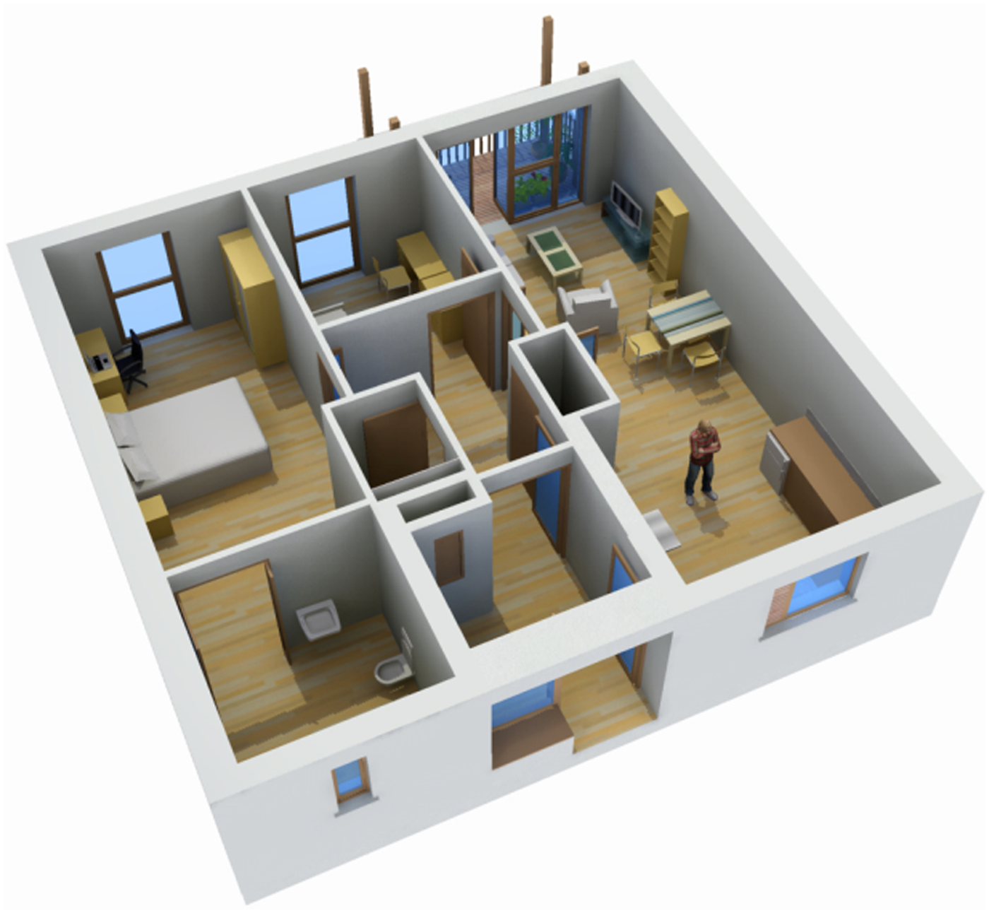
Typical Great Northern Haven home layout
Each presence sensor fired 155 times a day, on average, and the sensor firing times gave a characteristic that was easily identifiable by manual inspection. To help visualise behaviour patterns the sensor data was represented on a spiral plot called a ‘last clock’ which plots the data on a 24-hour clock with midnight at the top and spirals out from the centre. Each circuit represents a day (see Figure 2).
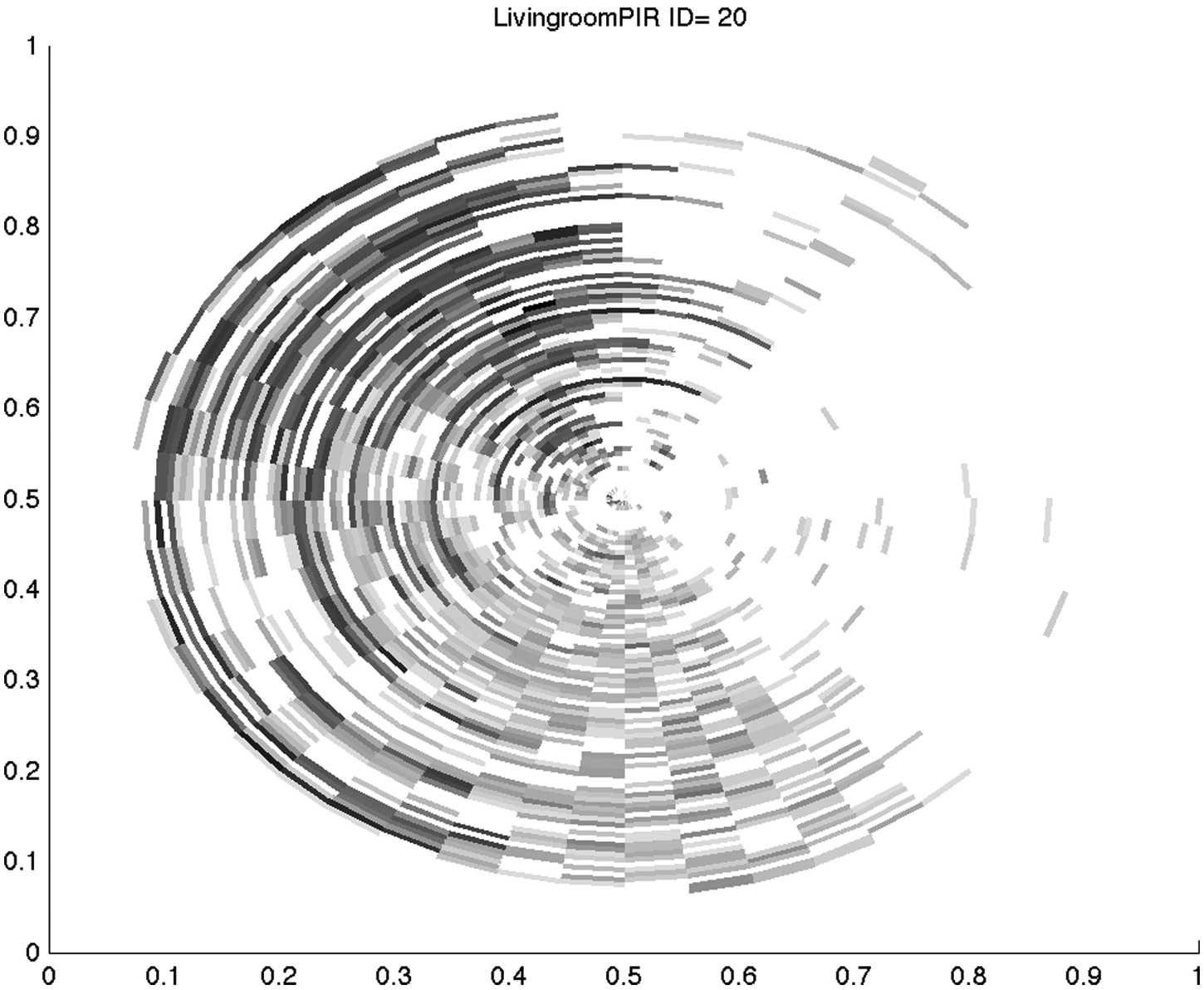
Living room presence sensor, showing most of the activity in the evening between 18:00 and 24:00
In Figure 2, 79 days of movement in the living room are displayed. Each circle represents a day of data with day one starting at the centre of the circle and day 79 at the outer circle. This resident rarely spends time in the living room between midnight and 9:00 and spends a lot of time in the living room between 18:00 and 0:00.
Methodology: Cluster analysis looking for similar homes
In order to find homes with similar movement patterns a cluster analysis was carried out with the data. The first complication that arose here is that all homes did not have the same number of days of data owing to the differing move-in dates. The home with the latest move-in date was used as the cut-off for the cluster analysis. All days earlier than this were omitted from the clustering. This meant that the clustering was carried out on 79 days of data. Each of those days was split into four equal time periods: 00:00–06:00, 06:00–12:00, 12:00–18:00 and 18:00–00:00. Four equal time periods were chosen as we wanted to capture resident’s general movement patterns throughout the day while allowing for large variation. The total number of times that the hall, bedroom and living room PIR sensors were triggered in each of these time periods was calculated. Hence, we were clustering on 948 values for each home. The cluster package in the R programming language 18 was used to carry out the analysis, employing both k-means and hierarchical methods.
When using k-means clustering the number of clusters must be known a priori and specified within the parameters of the clustering algorithm. In order to choose the best number of clusters we carried out the analysis with different numbers of clusters. We then graphed the silhouette plot 19 for each of these clusters. The silhouette coefficient of the point i, is defined as:
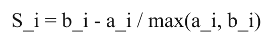
In this equation a_i is the average distance that point i is from all other points in the cluster to which is belongs and b_i is the smallest of the average distances of i to all clusters to which it does not belong. The silhouette coefficient for a cluster is defined to be the average over the silhouette coefficients of all points contained in the cluster. The silhouette coefficient for the entire data set is the average of the silhouette coefficients for all points in the dataset.
At the first step in the hierarchical algorithm each observation constitutes a cluster. At each step, the two closest clusters are joined to form a new cluster. Once an object has been assigned to a group it is never removed from the group later in the clustering process. The hierarchical method produces a complete sequence of cluster solutions beginning with n clusters and ending with one cluster containing all n observations. The proper number of clusters has to be selected.
At each step in the hierarchical algorithm we should join the two closest clusters. Our starting point is the dissimilarity matrix. It is easy to determine the two closest observations. Now a problem arises: how do we calculate the dissimilarity between one observation and one cluster or between two clusters? There are a large number of possible answers. In this analysis we use Ward’s method. 20 For each cluster, the means of all variables are calculated. Then the squared Euclidean distance to the cluster means is calculated. These distances are summed for all of the cases. At each step the two clusters that merge are those that result in the smallest increase in the overall sum of the squared within-cluster distances. We use a dendrogram to display the results of hierarchical clustering where the y axis indicates the relative difference between clusters.
Results
Cluster analysis: Looking for similar homes
The plots in Figure 3 show the results of the k-means clustering. With k-means clustering we do not know the best number of clusters to choose at the outset so we carry out the clustering with two, three, four, five and six clusters, and choose the result that produces the highest silhouette coefficients.The best clustering occurs in the case of four clusters where we get an average silhouette coefficient of 0.35 for the cluster home 4, home 5, home 12 and home 26. Each element except home 5 within this cluster has a silhouette coefficient above 0.3.
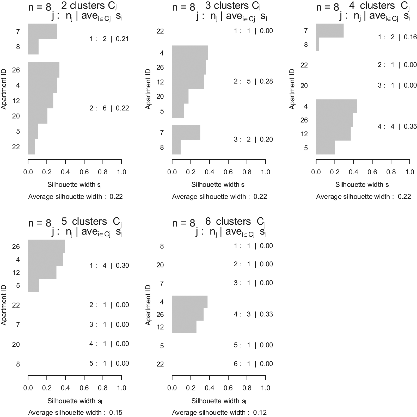
Results of k-means clustering using two, three, four, five and six clusters
Once again, Figure 4 shows that the only cluster of any significance is that containing home 4, home 12 and home 26. As was evident by the weak silhouette coefficient of home 5 in Figure 3 with n = 4, Figure 4 also suggests that home five is not part of the cluster with 4, 12 and 26. It suggests that homes 4, 12 and 26 are significantly different from one another, as we have to go a significant distance up the y axis before any clustering happens. This suggests that all homes have different patterns of movement and one model of movement behaviour will not fit all residents. It suggests that we will have to model residents individually.
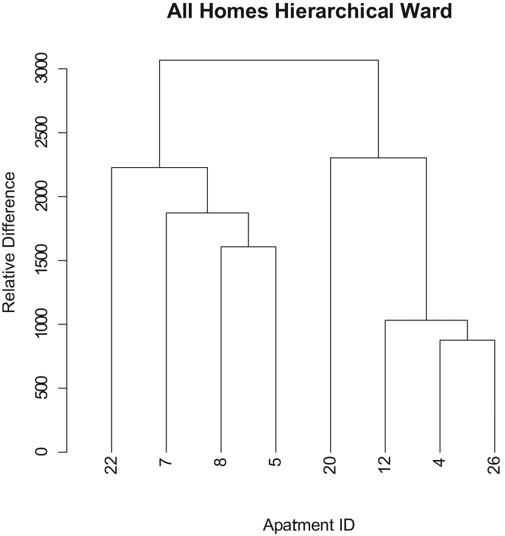
Dendrogram showing results of hierarchical clustering on all homes
Cluster analysis: Looking for movement patterns over days within homes
We also looked at each individual home and looked for patterns of movement over 79 days of data. Again, both k-means and hierarchical clustering were used to look for patterns. Each apartment had four different readings for each of the 3 sensors for 79 days. This data was used to cluster the days for each home.
Figure 5 shows the results of k-means clustering for home 7. There is quite strong evidence that this person has two distinct patterns in their movement throughout the house as the maximum silhouette coefficient is achieved when only two clusters are selected. One group of 28 days has a silhouette coefficient of 0.40 and a further group of 51 days has a silhouette coefficient of 0.40. It should be noted that the obvious interpretation of the 28 days being weekend days and the other 51 being weekdays is not the case. We need to carry out further interviews with the residents to investigate these results further.
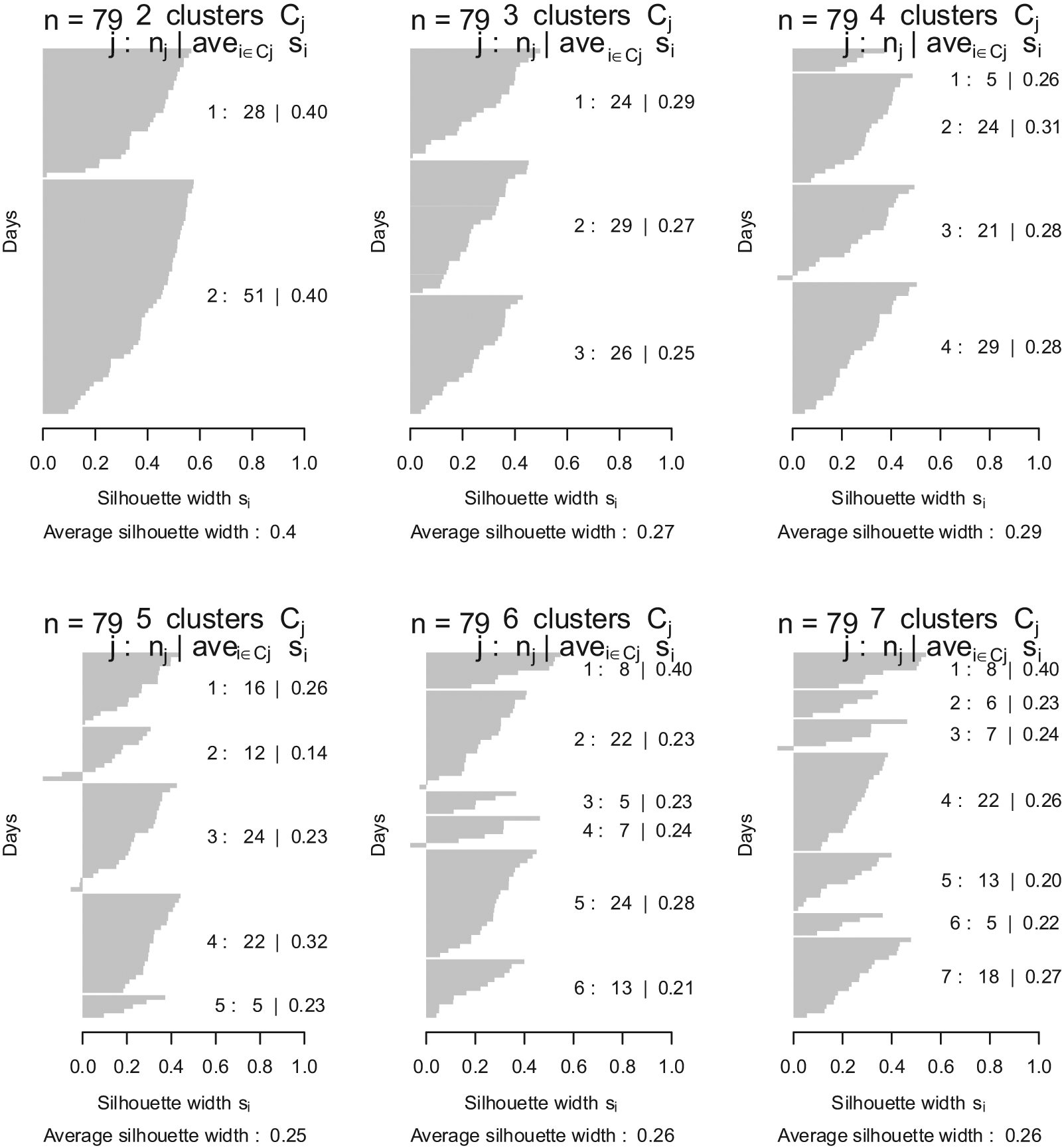
Results of k-means clustering with two, three, four, five, six and seven clusters for home 7
Once again, as seen in Figure 6, the results of the hierarchical clustering reinforce what the k-means clusters elucidated. Again, there is quite strong evidence that this individual has two distinct movement patterns throughout the house. This is good news for trying to model residents’ behaviour. While the between-home results tell us that we need a unique model for each individual, these results tell us that we only need to model two different types of movement.
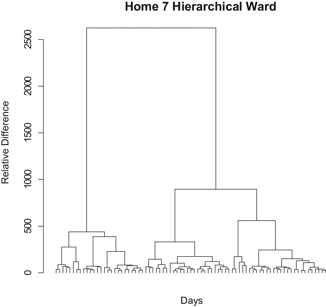
Results of hierarchical clustering over all days in home 7
Discussion
Cluster analysis: Looking for movement patterns over days within homes
The results shown in Figure 5 and Figure 6 show that both the k-means and hierarchical clustering methods give similar results. Both point to home 7 having two broad types of movement patterns. These two movement patterns are very dissimilar from each other.
All seven other homes in the analysis showed a similar pattern of having two distinct movement types. A resident’s level of routine is evident from how well the days cluster.
Further work is required to validate these clusters and to understand their meaning for each resident. We intend to ask residents to fill out a daily survey that will help us to gather the required ground truth data to interpret these results. Once this has been done we hope to use these two different types of days to monitor the resident for days that are dissimilar to either of these two clusters.
Conclusion
The cluster analysis between individual homes reinforces the idea that each home has distinct movement patterns. Only one relatively weak cluster of three homes was found.
The cluster analysis within each home yielded the most surprising results. Each of the eight homes clustered best when only two clusters were chosen for the k-means clustering. This was reinforced by carrying out the analysis using hierarchical clustering and studying the associated dendrograms. The clustering suggests that all eight homes have two distinct movement patterns. Some homes have much stronger clustering than others, suggesting that they have a stronger routine and, hence, that their movement patterns are more similar from day to day.
This work has clear practical implications for the design of behaviour models to monitor assisted living environments. The first between-home clustering tells us that there is no ‘one size fits all solution’. Each home in our study has a distinct movement pattern and our future designs need to take account of this individuality.
That first seemingly negative, but not unexpected, finding is tempered by the second, more positive, finding that there is strong routine in the movement within homes. Each home showed two distinct patterns of movement. In future work we aim to gather ground truth data to validate these two clusters. Having done that, we will fit distributions to represent the two different clusters and use these as a measure of normal behaviour against which future days can be compared.
We hope that these results can be applied more generally to other features. If we cluster on the feature (movement in this article) and find that there are n clusters then we will first validate these clusters against ground truth information gathered by asking the residents about their daily activities and then generate n distributions which will act as a measure of normal behaviour. If a future day is suitably far away from one of these n distributions it could trigger an alert. If one of these n distributions turns out to model when the resident was ill or in decline it can be used to recognise this behaviour again in the future. Identifying these behaviours reliably and comparing them to temporal health conditions will allow us to predict in the future, from the behaviour alone, when a resident is showing signs of decline and allow us move to intervene.
Footnotes
Funding
The CASALA research centre at the Dundalk Institute of Technology is funded by an Enterprise Ireland Applied Research Enhancement Centre Programme.