
Abstract
Effective building energy management (e.g. temperature control strategies) necessitates reliable and computationally efficient building thermal models. One type of them is the resistor–capacitor (RC) model. However, estimating model parameters and inputs (e.g. solar heat gain) simultaneously is challenging, especially when some of the temperature states are missing due to instrumentation limitations and/or sensor malfunctions. The present study utilizes unscented Kalman filter (UKF) and nonlinear least squares (NLSs) methods for parameters and input estimation of RC models with possible unavailable temperature states. The estimation procedure, mathematical operations and result analysis are presented in detail. To evaluate the capability of the method, two case studies were conducted. The first case study involved a simple, made-up RC model with known parameters, inputs and states, while the second case study used monitored data from a single detached house. The capability of the method was evaluated by comparing the estimated parameters, inputs and states to the corresponding true values in both study cases. The performance evaluation shows that the proposed method can effectively estimate RC model parameters and inputs, even with certain missing states. The proposed method can be employed for timely online updating of RC model parameters to improve response prediction.
Keywords
Introduction
Buildings currently consume approximately 40% of global energy and contribute to 31% of world CO2 emissions 1 ; therefore, reducing buildings’ energy consumption is critical to meeting global sustainability targets.2,3 Amongst the efforts to reduce buildings’ energy consumption, building energy management with control systems that can optimize building energy consumption is being developed and deployed.4,5 These systems are proven to have the potential to save energy by up to 28%. 6 Control systems require reliable thermal dynamic models in order to estimate buildings’ thermal parameters (e.g. effective thermal resistance) and behaviour (e.g. temperature response). 4
Different modelling strategies, including ‘white-box’, ‘black-box’ and ‘grey-box’ modelling, have been developed in the literature to predict the thermal behaviour of buildings and their systems.7–11 White-box (physics-based) modelling, such as using Energy Plus, 12 requires detailed construction information (e.g. dimensions) and can simulate building physics in detail. 13 Due to the unknowns of building conditions (e.g. material degradation, users’ behaviour and operation strategies), using this modelling strategy on existing buildings can be problematic. 12 On the other hand, black-box modelling uses pure mathematical machine-learning techniques, such as using artificial neural network,14,15 to create non-interpretable (hidden) relationships between input and output data without necessitating physics. 16 Black-box modelling requires a large amount of high-quality data. 17 ‘Grey-box’ modelling strategy, such as thermal resistor–capacitor (RC) models, is based on a physics-base model structure and uses mathematical optimization techniques to estimate the equivalent physical parameters of the model. The strategy incorporates the benefits of both white-box to eliminate outliers and that of black-box strategies to reduce the necessity of detailed information. The grey-box modelling approach has been widely used for thermal dynamic modelling.18–22
RC models are based on a set of equivalent model parameters, resistors (Rs) and capacitors (Cs), to relate system inputs (e.g. heating and cooling supply) and temperature states. 23 The model parameters can be influenced by both internal and external factors. Internal factors include people, furniture and electric consumption, while external factors encompass adjacent obstructions, air infiltration and weather-related influences. Thus, RC model parameters are not meant to be directly measured or calculated simply based on the construction details of buildings. The unknown parameters and inputs can be estimated through calibration with measured data (usually temperature states).23–25
RC model parameter estimation is typically an inverse optimization problem, which can be solved by various algorithms (e.g. genetic algorithms, 26 least squares regression system identification, 27 stochastic filtering, 28 linear Kalman filter, 29 extended Kalman filter, 28 ensemble Kalman filter 30 and unscented Kalman filter (UKF) 25 ). Using an extended Kalman filter and UKF with low-sampling-rate historical data, Baldi et al. 31 estimated the unknown states and parameters of a simple RC model. Later on, Li et al. 25 demonstrated the capability of UKF to jointly estimate the unknown states and model parameters in complex RC models representing real-life buildings. Additionally, Zamani et al. 21 introduced a novel method integrating RC models and UKF with nonlinear least squares (NLSs) for precise estimation of heating and cooling supply, essential for effective temperature control in buildings. Through case studies, its accuracy in estimating supply was demonstrated, affirming its suitability for temperature control objectives.
Parameters can be obtained via offline estimation (i.e. batch) assuming the parameters are constant within the period of a set of collected measurements and using the measurements to estimate the parameter. This approach may result in inaccurate estimations and consequently inaccurate predictions due to time-variant building physical conditions and occupants’ behaviours.28,32,33 To address this issue, parameter estimation can be conducted in an online manner (e.g. adaptive), in which the model parameters are updated continuously with new measurements in a computationally efficient manner.25,34–36 There are various online parameter estimation methods in the literature, including recursive least square, 37 recursive prediction error minimization, 38 linear Kalman filter, extended Kalman filter and UKF. Numerous studies in the literature have employed the Kalman filter methods to demonstrate how RC models and the Kalman filter can work well together for online parameter estimations.25,39 In particular, Radecki et al. 39 demonstrated that temperature predictions are accurate when UKF is used to estimate the parameters of a multi-zone thermal RC model. Later on, a framework was proposed by Maasoumy et al. 40 for an online building model that simultaneously estimates the states and unknown parameters and continuously tunes the model parameters. In another study, extended Kalman filter was applied to an RC model of a passive house 28 to create an online thermal model that can accurately predict indoor temperature states.
The abovementioned parameter estimation work focused on cases where all system inputs (e.g. heating and cooling supply) are known; however, in real practice, system inputs and even some temperature states may be unknown for various reasons. For example, the system inputs and states can be temporarily missing due to sensor malfunction or unavailable due to limitations in practices (e.g. too difficult to obtain accurate data) and resources (e.g. too expensive to install many sensors). Meanwhile, knowing the inputs is crucial to the optimization of control strategies. For example, knowing the actual capacity of space heating/cooling supply and solar heat gain is critical to developing predictive control strategies (e.g. space preheating and cooling). This study aimed to develop a method to jointly estimate model parameters and unknown inputs. Through examples, the capability of the developed method was evaluated for estimating unknown model parameters and inputs in different scenarios with different numbers of available temperature states.
Problem statement and methodology
In practice, some inputs of a building’s thermal system can be unavailable, immeasurable, or difficult to measure for various reasons, as mentioned earlier in the Introduction section. Therefore, there is a need to estimate both unknown RC model parameters and inputs. One approach to doing so is to use available system temperature state measurements. Furthermore, it is not often that all the system states are measured and/or can be easily measured, and thus some of them may also be unknown. Accordingly, this study developed a feasible method that can be used to estimate model parameters and unknown inputs with possibly missing states, as illustrated in Figure 1. The missing states can also be simultaneously estimated by the proposed method. The development of a suitable model structure (i.e. number of temperature nodes, inputs, R, C and their connections) is beyond the scope of this study and, therefore, is not discussed in this paper. After obtaining a suitable model structure, the RC model parameters, inputs and possibly unavailable states were estimated using a UKF-based parameter-input estimation method integrated with NLS.41–43 Specifically, the UKF was mainly used for parameter and state estimation, while the NLS was used to estimate unknown inputs. This section presents the two essential components of the developed method: (1) thermal dynamic modelling using RC models and (2) a parameter-input estimation method developed based on the integration of the UKF and NLS. General procedure of the proposed parameter-input estimation method.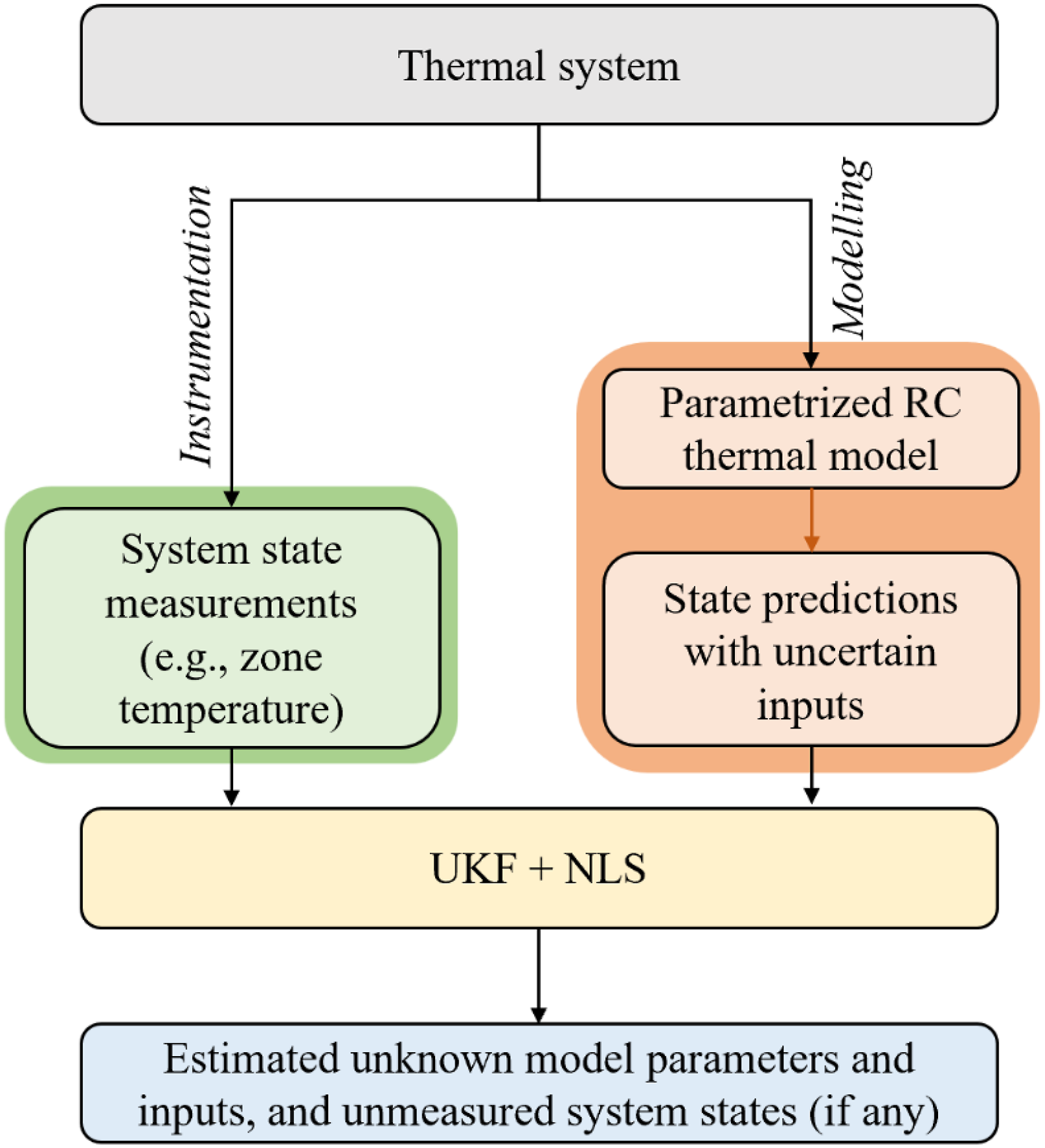
Thermal dynamic modelling using RC models
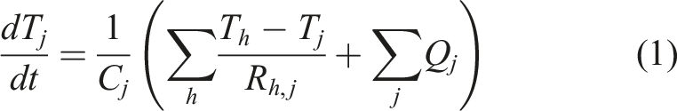
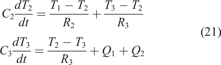
In using an RC model to model the thermal dynamics of a building’s thermal zone, the temperature nodes within the zone can be represented by model nodes. Then the model nodes are connected to model parameters (i.e. Rs and Cs) and inputs (e.g. solar heat gain or mechanical heating/cooling supply). The model nodes are connected to each other through the Rs. The parameters, inputs and model nodes together create a thermal RC network. Running the RC model with inputs (i.e. simulation) can provide temperatures at the model nodes (i.e. states). The thermal dynamics at each node can be presented by ordinary differential equations (ODEs). The typical equation for a node, say

Parameter-input estimation method
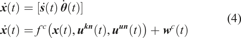
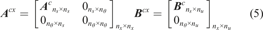
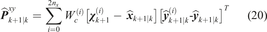
This section describes the method for estimating unknown model parameters, inputs and unmeasured states, if any, using the UKF integrated with NLS. The model parameters were grouped to form a vector of parameters, denoted by

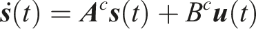
After considering additive process noise, which represents the estimation error, equation (3) can be transformed to a state-transition equation in the state-space format as shown in equation (4):

Corresponding measurements of the system states can be linked to predictions from the thermal dynamic model through the measurement equation as shown in equation (7):

Using discretely monitored system states (i.e. node temperatures) to estimate unknown thermal dynamic model parameters and inputs necessitates an estimation method dealing with the nonlinear discrete-time state-space model. In this regard, the UKF method was selected for parameter and state estimation because it has been proven to be robust and effective for highly nonlinear problems.43,45 Furthermore, to efficiently estimate the unknown model inputs, the NLS algorithm was integrated into UKF. The combination of UKF and NLS allowed the estimation of unknown model inputs and parameters, together with unmeasured states.41–43
UKF is a Kalman-based technique, employing a prediction–correction two-step strategy based on unscented transformation (UT).
46
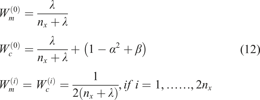
In the prediction step, UT estimates the mean and covariance matrix of the nonlinear state function by evaluating the function using a set of deterministically selected points, known as sigma points (SPs). The unscented transformation requires a selection of
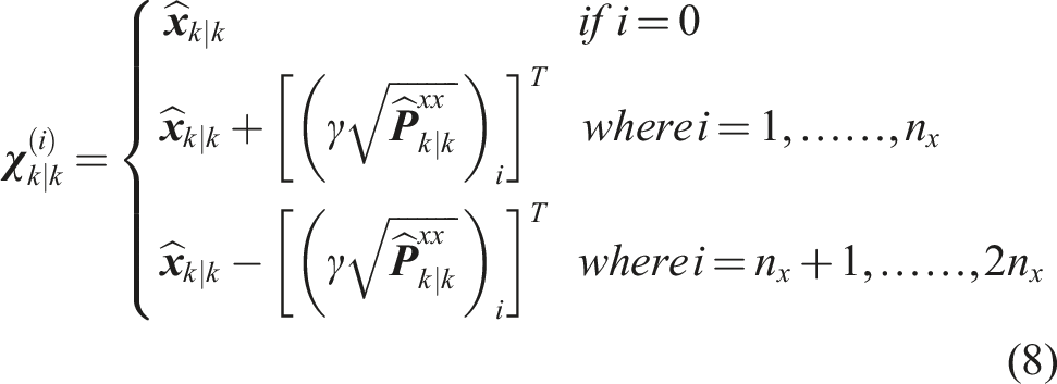
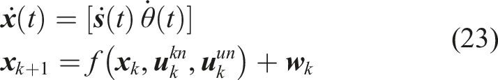
By using the initially determined SPs (i.e.

In order to estimate the unknown model inputs, the developed method works as an optimization tool to minimize the estimation error (i.e.

Therefore, by adjusting the unknown inputs for minimizing estimation error (i.e.
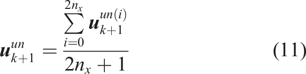
Once the unknown model input was estimated and SPs weighting coefficients were calculated, the prior estimates for the mean vector
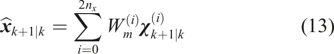
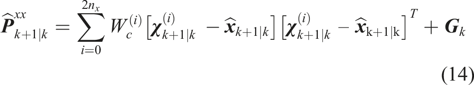
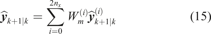
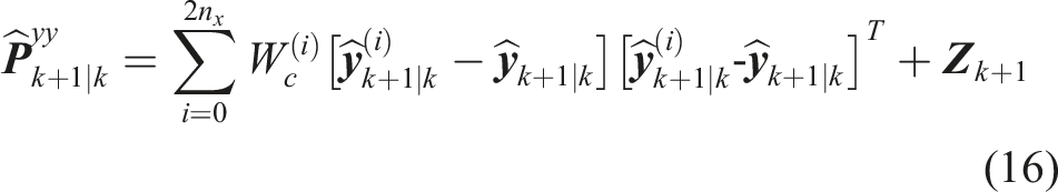
Then, the predicted mean and covariance matrices of the measurement vector at time step k + 1 can be determined by equations (15) and (16):
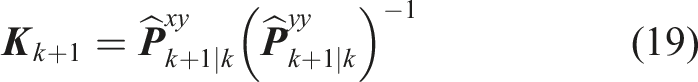
At time step


To summarize, Figure 2 presents a flowchart for the developed method that can be used for parameter and input estimations in cases with unknown model inputs and unmeasured states. Parameter-input estimation method based on UKF integrated with NLS.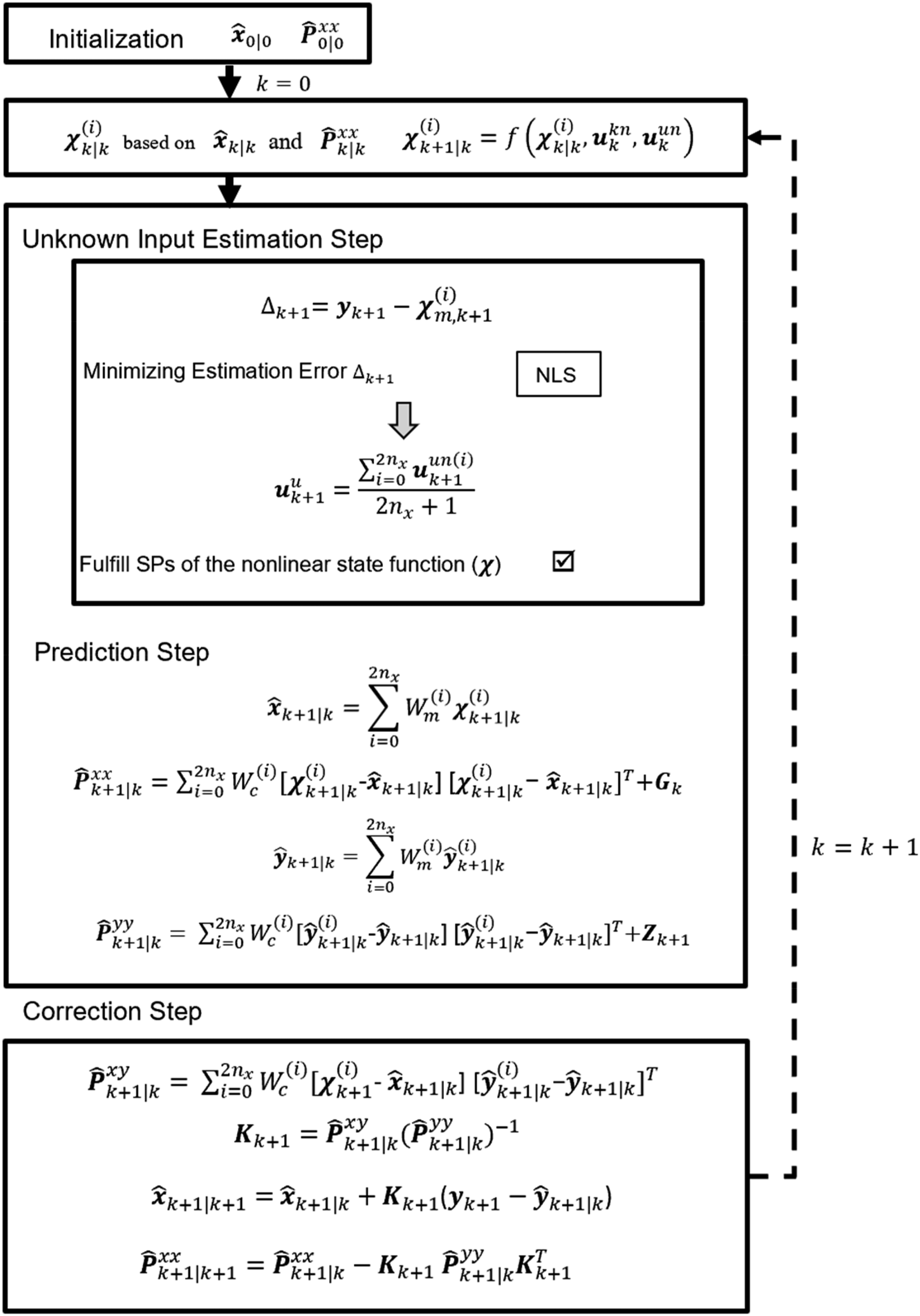
Application examples
Two case studies are presented to illustrate and evaluate the developed method: (1) one simple made-up RC model consisting of two thermal resistors and two thermal capacitances (i.e. 2R2C), for which simulated responses were considered as measurements, and (2) one real-world single-family house with noticeably more complexity (10R6C) and real-world recorded data. The capability of the method was evaluated by comparing the estimated parameters, inputs and states to the corresponding values in both study cases.
A case study with a made-up RC model
The made-up RC model, labelled as 2R2C, is shown in Figure 3. This model consists of four model parameters, two thermal resistors (i.e. R2 and R3 in 2R2C model. 2R2C made-up model inputs.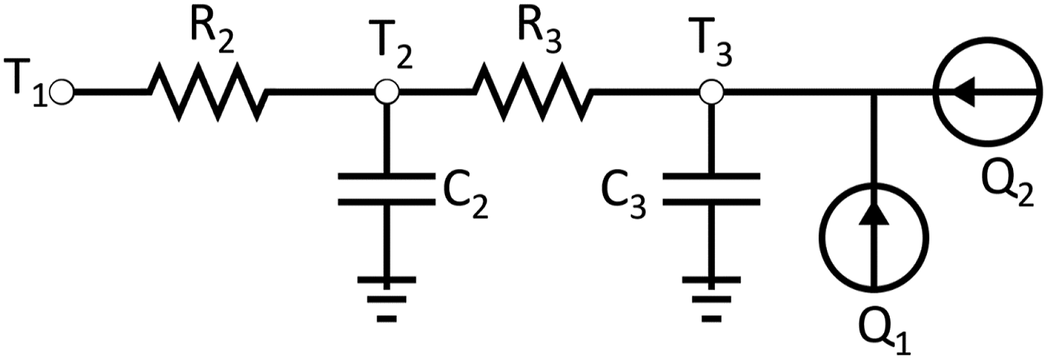
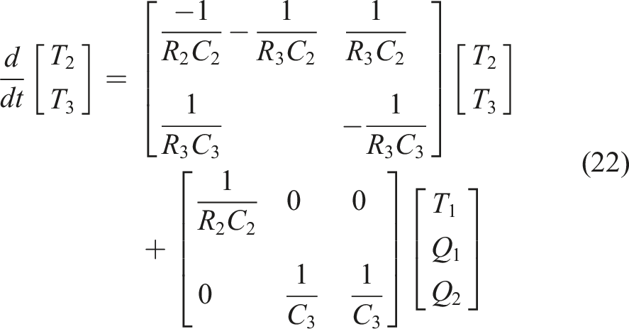
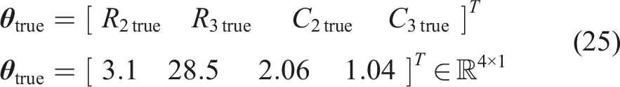
The ordinary differential equations and state-space form of this RC model are shown in the equations (21) to (23), and the made-up (true) model parameters are shown in equation (25). To generate responses (i.e. states), the discrete-time linear state equations of the model were derived based on the true model parameters and then run with made-up inputs. The simulated responses (i.e. temperature states) were considered the true states in this study, and then they were contaminated by adding white Gaussian noise to generate measured states. The noise has a mean of zero and a standard deviation of 0.16
Accordingly, the state-space equation of the 2R2C model, when Q2 was assumed to be unknown, can be written as equation (22) and the discretized form is described by equations (23) and (24):
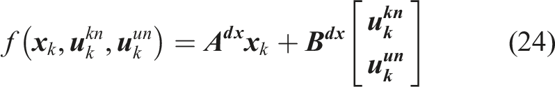
where
Hourly data
51
(true inputs and states) were generated for 1 month (i.e. 720 h). The first 540 h of data were used for estimation and evaluation purposes, while the final 180 h of data were employed to evaluate the prediction accuracy of the calibrated model, which used the model parameters estimated at the end of the 540 h estimation period. The allocation of hours in each dataset was substantiated by prior studies23,25 indicating the sufficiency of 540 h for capturing crucial thermal dynamics, ensuring the methodology is aligned with established practices and empirical findings. Furthermore, dedicating 180 h to prediction evaluation is in accordance with the requirements to demonstrate the model’s predictive capability effectively.
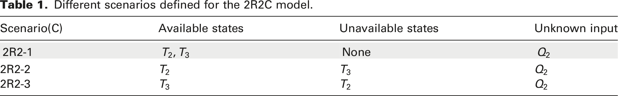
Different scenarios defined for the 2R2C model.
The state vector of this RC model is defined by 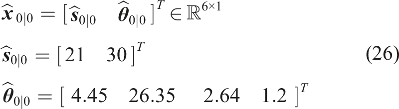
Figure 5 presents the time histories of model parameter estimation for Scenario 2R2C-1, where all the states were measured. In these figures, the dashed black line shows true model parameter values, and the red line shows the mean estimate. The shaded grey area shows the mean +/− two standard deviations obtained from the covariance matrix Time histories of model parameter estimations for scenario 2R2C-1: (a) thermal resistance and (b) thermal capacitances. Last estimated model parameters for scenarios 2R2C-2 and 2R2C-3.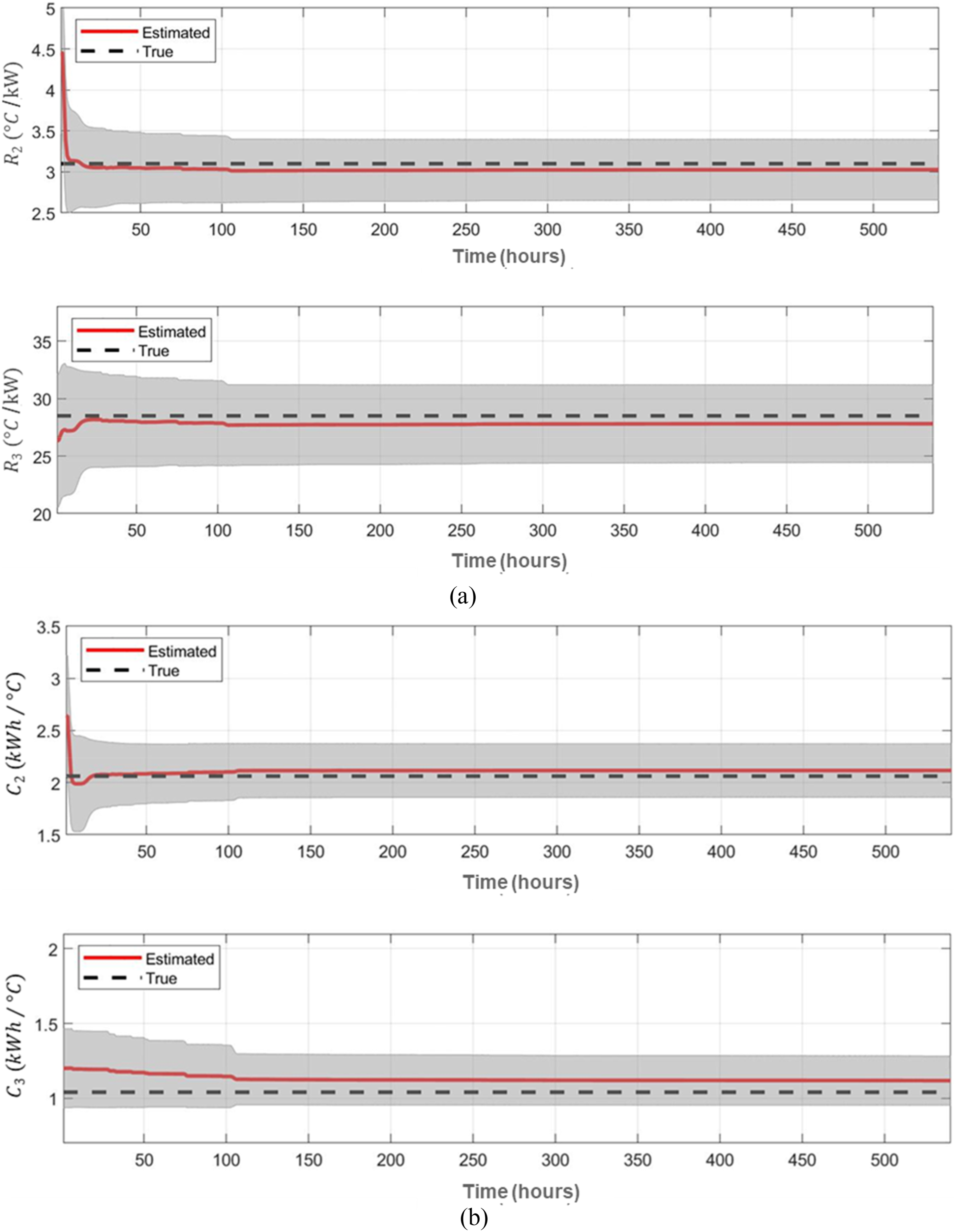
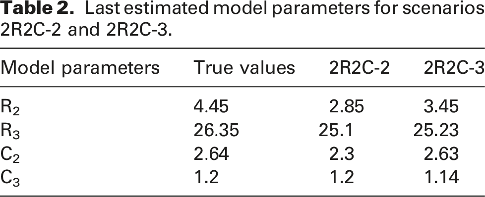
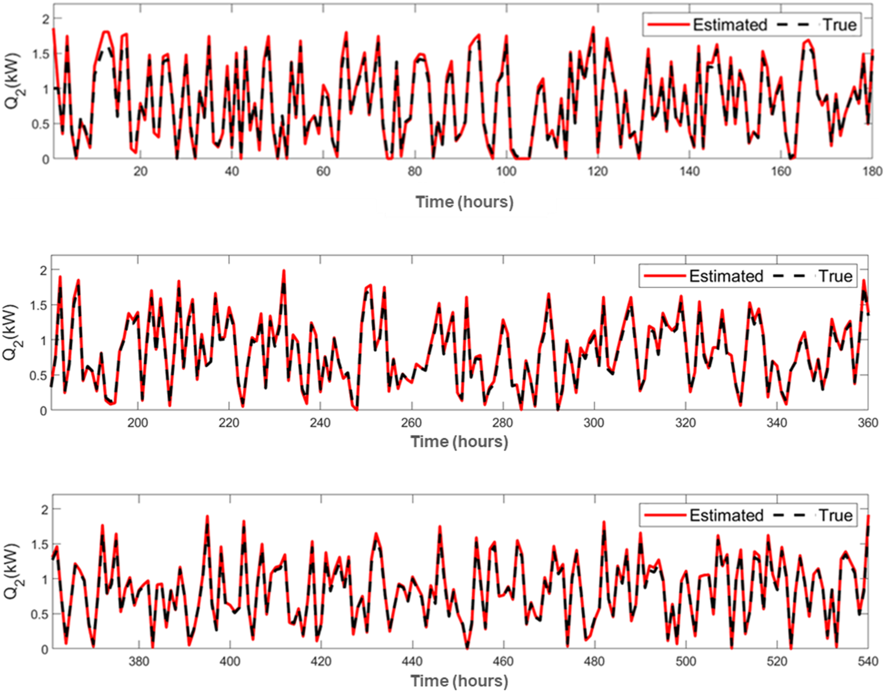
Figure 6 presents the estimation history of the unknown model input Comparison between the true and estimated model input for scenario 2R2C-1.
Using the developed method, parameters, input and states were estimated at each time step of the estimation period. Figure 7 compares the estimated and the true profiles of the two states of the 2R2C model (i.e. T2 and T3) in Scenario 2R2C-1. The MAPE of the estimated state and the true one for both temperatures were 0.4% and 0.82% for T2 and T3, respectively, which indicates excellent agreement between the estimated results and the corresponding true states. The accuracy of the estimated T3 is not as high as that for T2. This is due to the unknown input, Q2, in the estimation period being linked to T3, as shown in Figure 3. Figure 7 also shows that the developed method is able to estimate the parameters, inputs and states relatively accurately within the first few time steps. This observation indicates the suitability of the method for online estimations. Comparison between true and estimated temperature responses for Scenario 2R2C-1.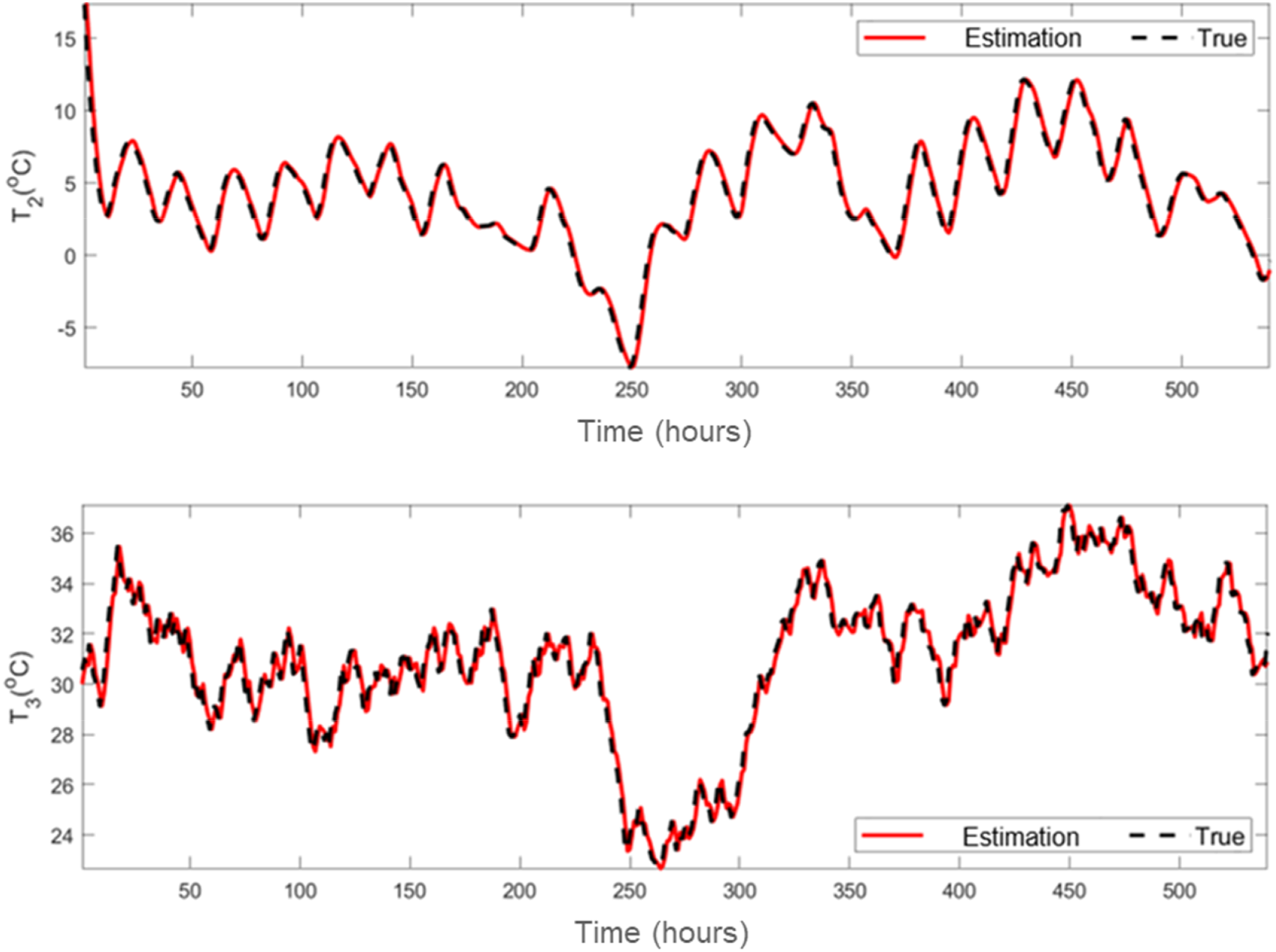
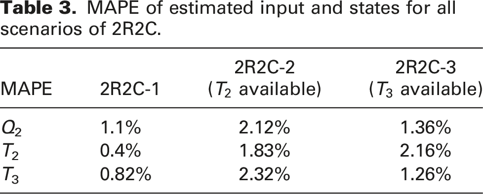
MAPE of estimated input and states for all scenarios of 2R2C.
Using the parameters obtained at the end of the 540-h estimation period, the RC models were used to simulate the states in the prediction period (with known inputs). The predicted temperature responses were generated at each time step, hourly from hours 541 to 720. Figure 8 compares the predicted temperature responses for Scenario 2R2C-1. Both temperature responses T2 and T3 were predicted with good accuracy, with the MAPE values being 0.92% and 2.55%, respectively. Again, the accuracy of the predicted response for T3 was not as high as that for T2, due to the unknown input, Q2, in the estimation period linked to T3, as shown in Figure 3. This comparison indicates that the inaccuracy in the parameter estimation would not result in a significant error in state prediction; therefore, the developed method is sufficient for the analysis of building thermal dynamics when all states are measured. Comparison between true and predicted temperature responses for Scenario 2R2C-1.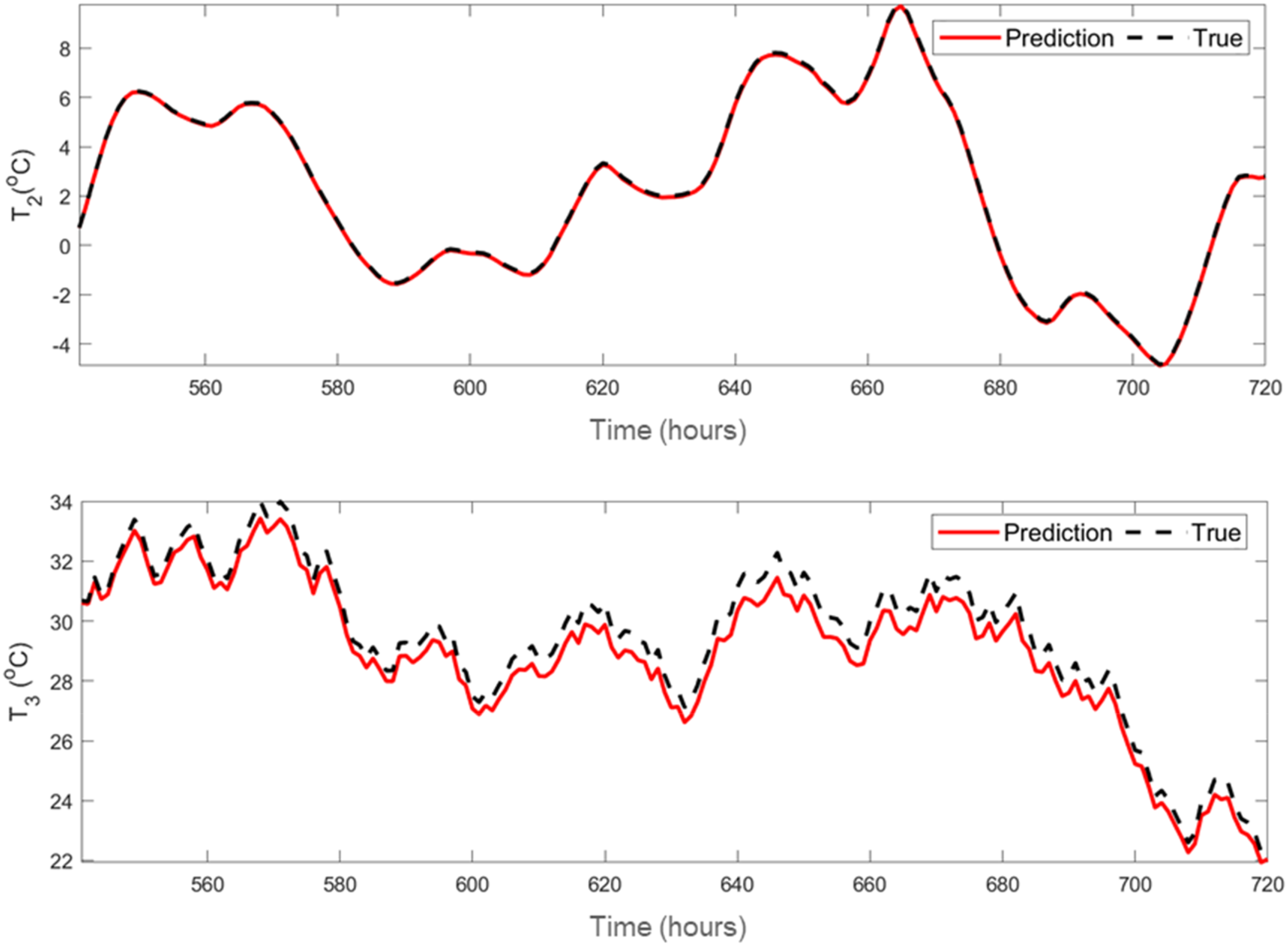
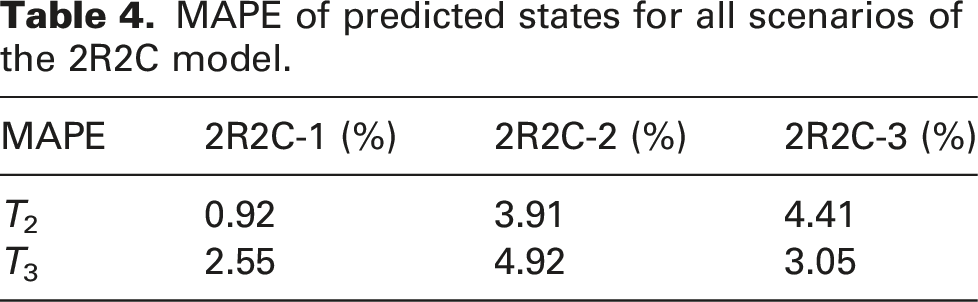
MAPE of predicted states for all scenarios of the 2R2C model.
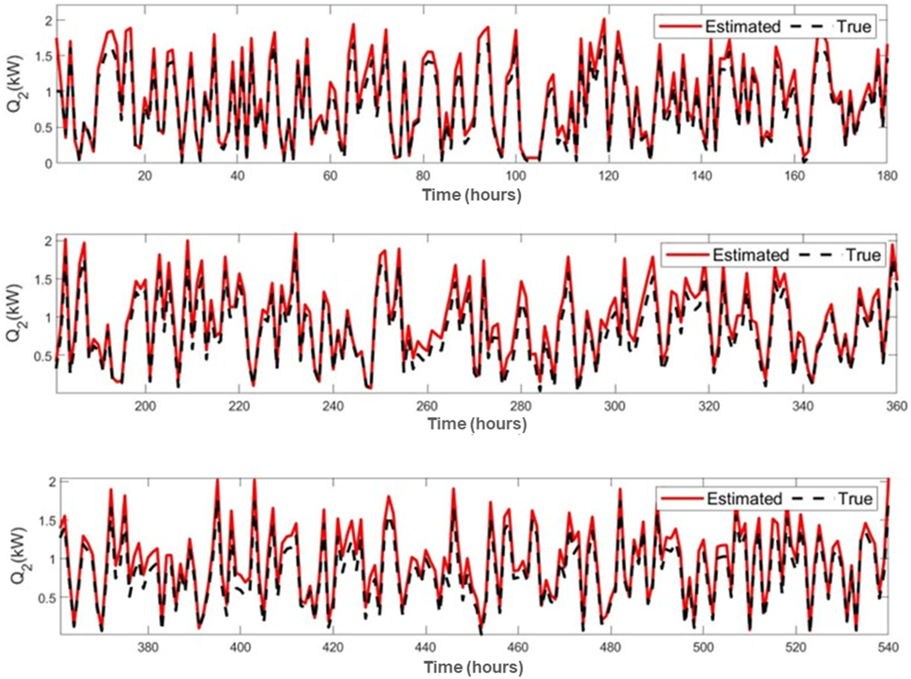
Comparison between true and estimated model input for scenario 2R2C-2.
Comparison between true and estimated temperature responses for scenario 2R2C-2.
Comparison between true and estimated model input for scenario 2R2C-3.
Comparison between true and estimated temperature responses for scenario 2R2C-3.
A case study with a real-world house
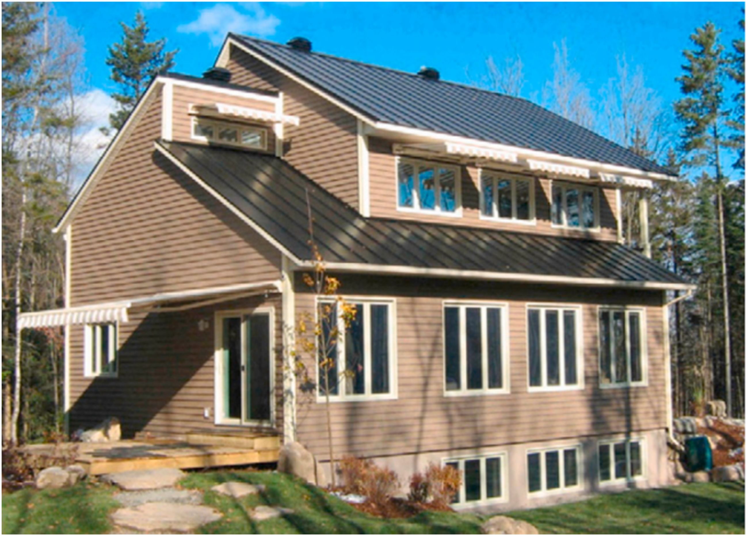
The developed method was tested in a real-world low-energy wooden-frame house in Eastman, Quebec, Canada, as shown in Figure 13.
26
The study used 720 h of measured data. The first 540 h of data, organized on an hourly basis, were designated as the estimation dataset, and the remainder as the prediction dataset. The allocation of hours in each dataset was supported by previous studies,23,25 which demonstrated the adequacy of 540 h for capturing essential thermal dynamics. This ensures that our methodology is consistent with established practices and empirical findings. Various scenarios were defined based on the availability of different state measurements. Accordingly, the effectiveness of the developed method was evaluated by (1) comparing the estimated values of states and input with their measured (true) values in the estimation dataset and (2) comparing the predicted responses obtained using the final estimated model parameters with the measured responses in the prediction dataset. A single detached house as a case study.
26
The RC model structure of the detached single-family house shown in Figure 14 was developed by Wang et al.
26
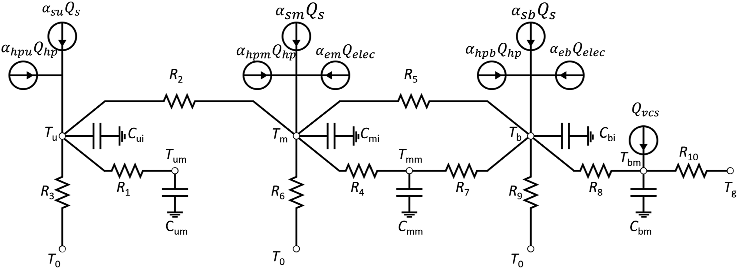
In this RC model, the basement, second floor and main floor were labelled as b, u and m, respectively. This RC model was called 10R6C, as it consists of 10 thermal resistances and 6 thermal capacitances, T
m
, and T
b
in °C were the zone temperatures of the second floor, main floor and basement, respectively. T
um
, T
mm
and T
bm
were the internal thermal mass temperature responses, which were not measured. The ordinary differential equations and state-space form of this RC model are shown in equations (28) and (29). RC model structure for the single detached house.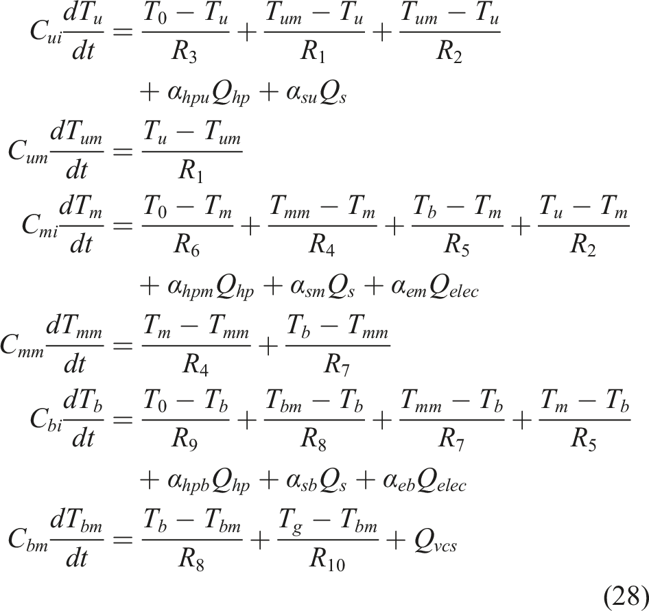
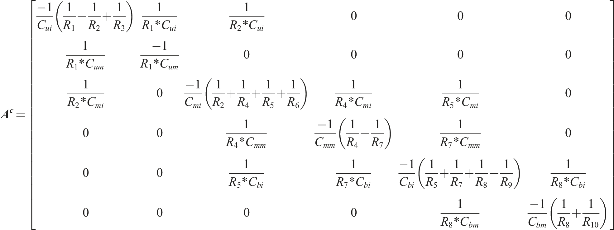
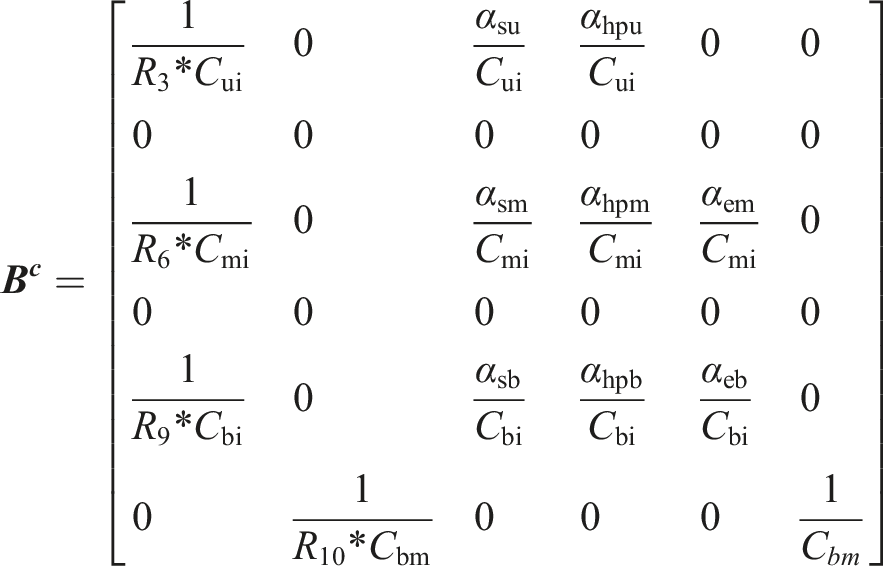
Therefore, the state-space form of the 10R6C model can be written as follows: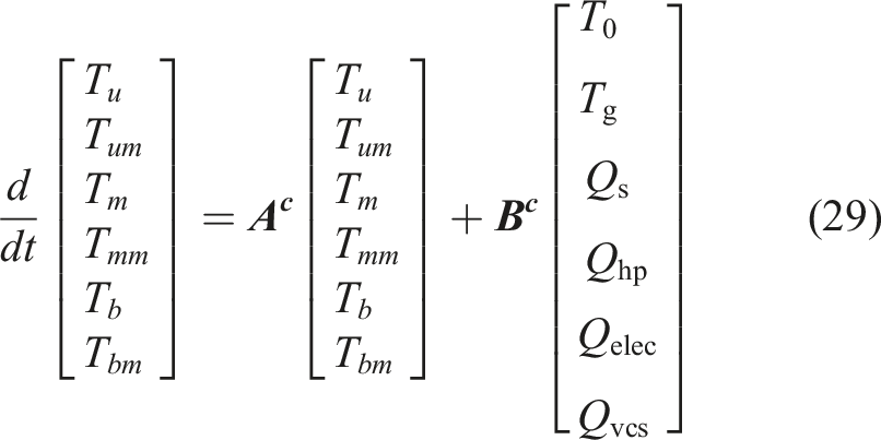
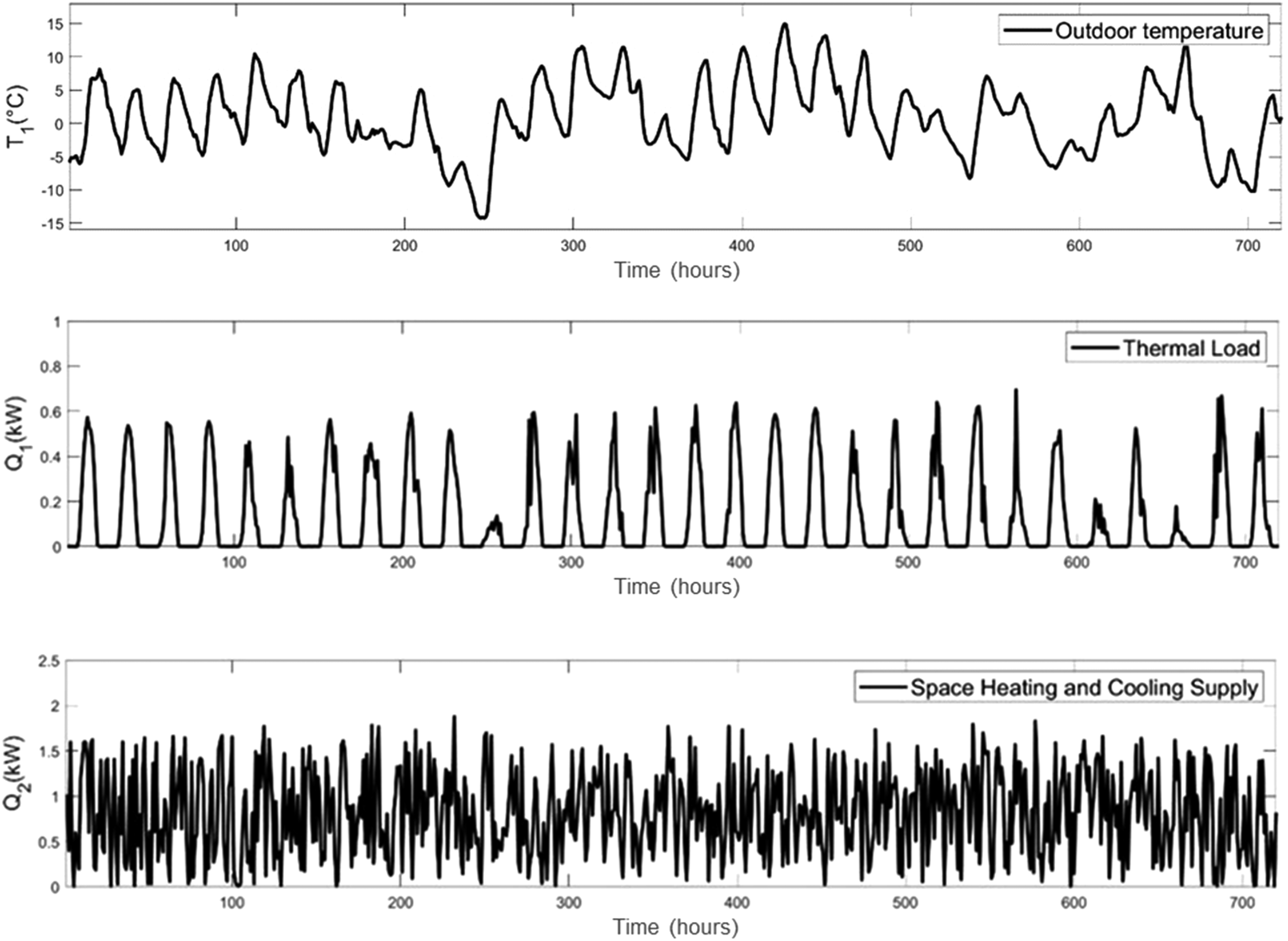
The hourly model inputs for this RC thermal model are shown in Figure 15. The model inputs include (1) global irradiation Q
s
in kW per unit area on the south facade, which was used to obtain approximate effective solar heat gains weighted by solar gain factors ( 10R6C model inputs.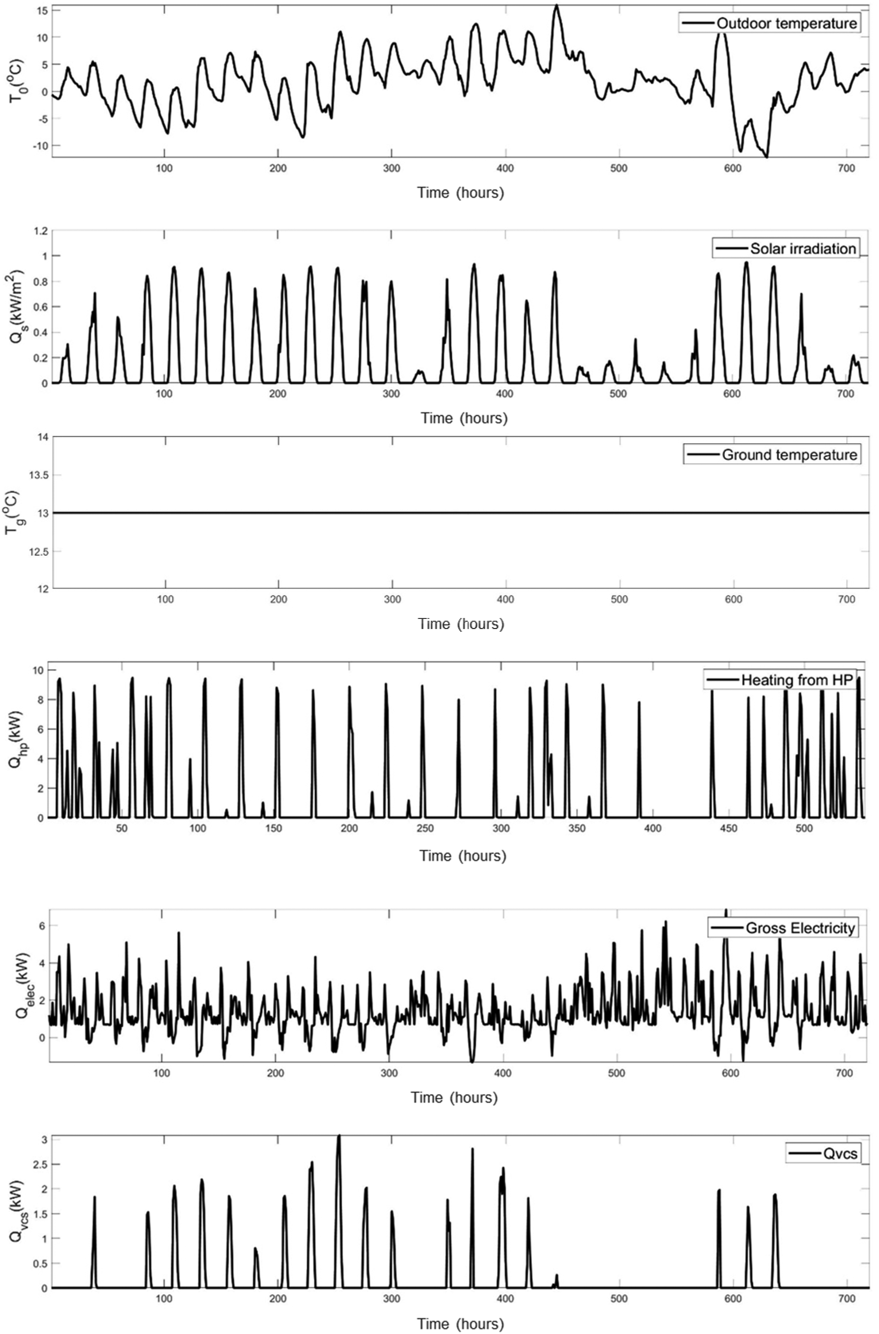
The state vector of this RC model can be defined by 

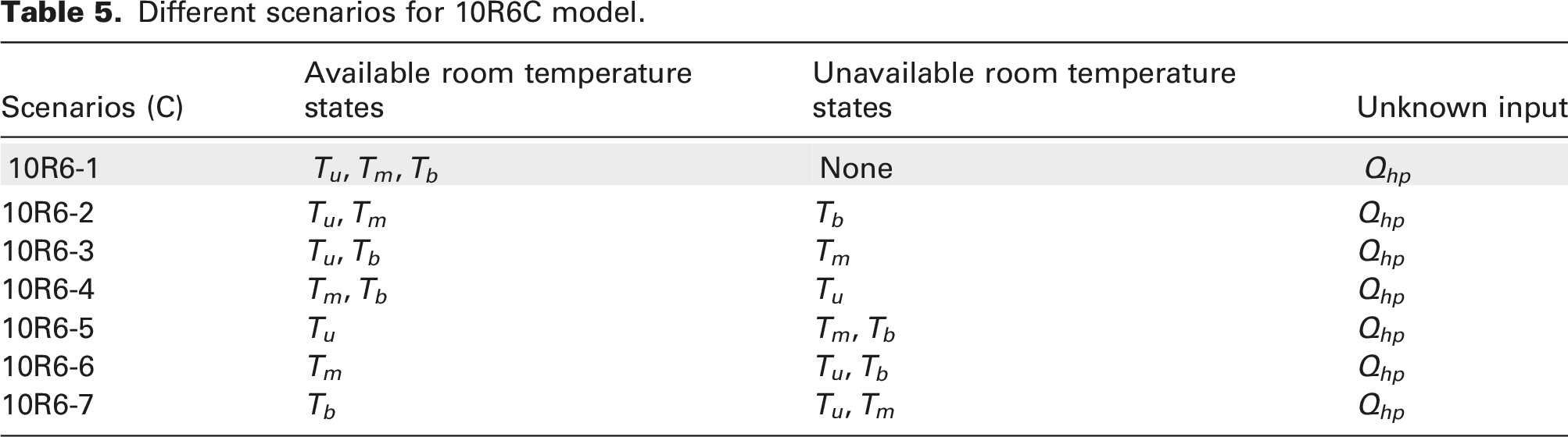
Different scenarios for 10R6C model.
In the estimation phase, the initial mean estimates for the state-parameter vector can be expressed as equation (33):


As explained in the case study of a simple RC model, the diagonal terms for the states
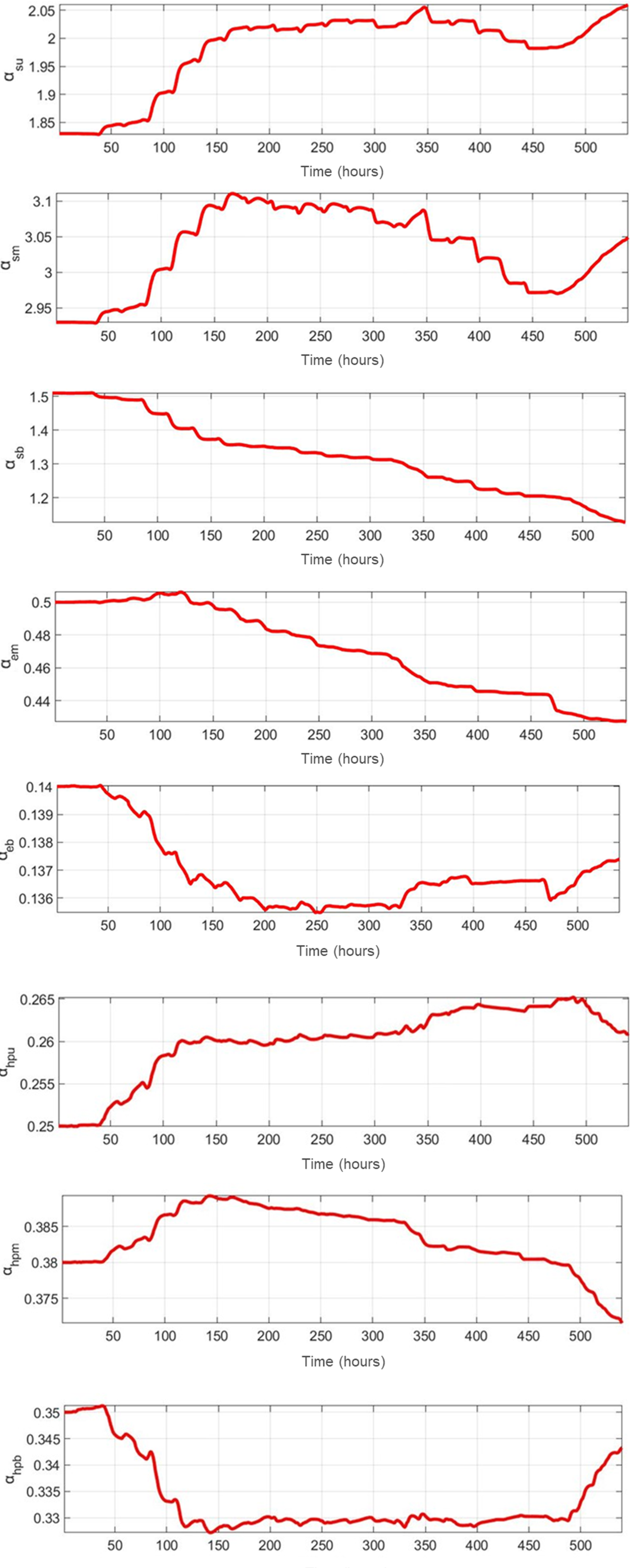
The results of the estimation of model parameters, including thermal resistances ( 10R6C model parameters estimation: thermal resistances for scenario 10R6C-1. 10R6C model parameters estimation: thermal capacitances for scenario 10R6C-1. 10R6C model parameters estimation: solar and internal gain factors for scenario 10R6C-1.
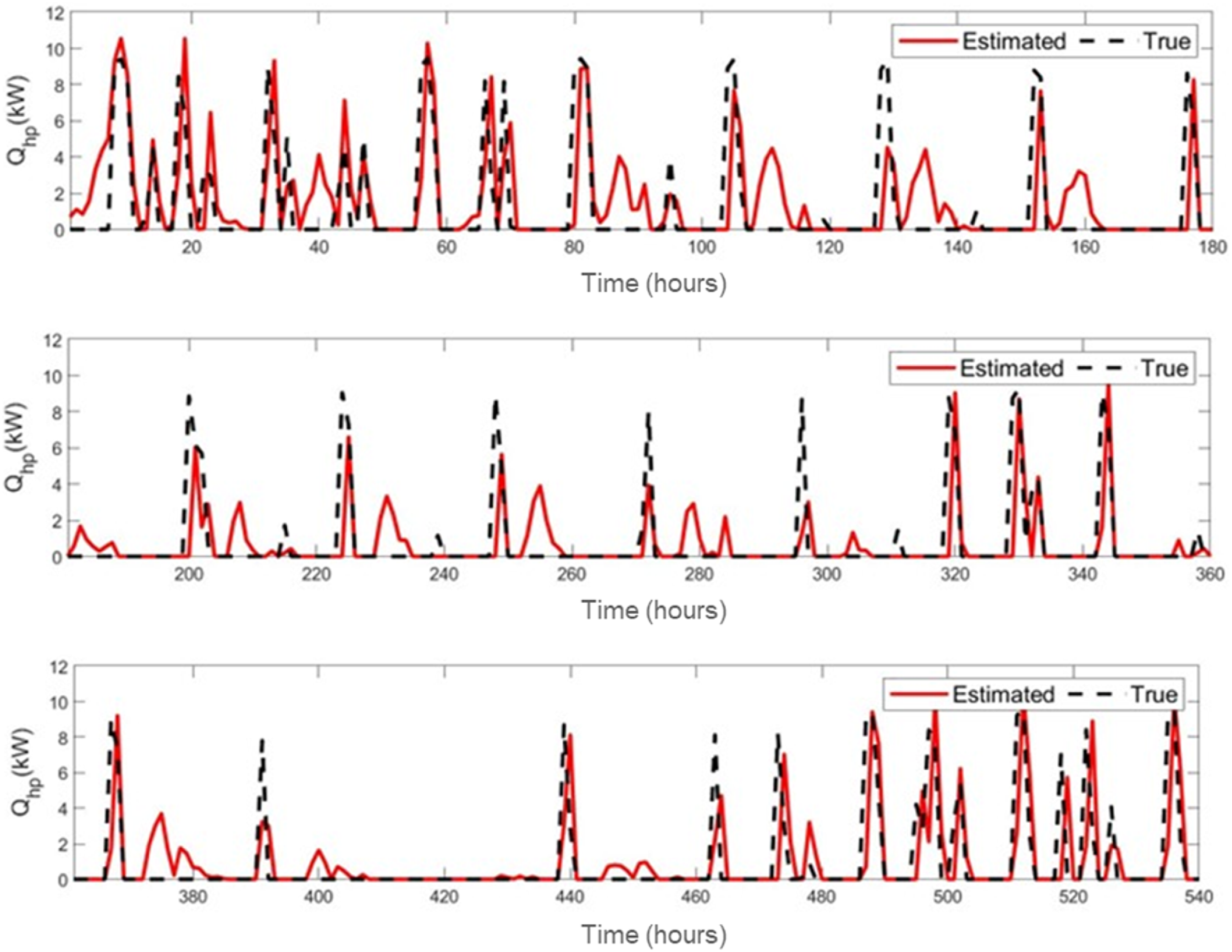
The performance of the developed method in estimating the model input is demonstrated in Figure 19, which compares the estimated model input Q
hp
to its true value in Scenario 10R6C-1. To illustrate the estimation results more clearly, the 540 h of time histories were divided into three 180-h segments, which is shown in Figure 19. The MAPE of estimated input was about 10%. Notably, there were specific time periods where Qhp experienced both overestimations and underestimations. A significant contributor to these fluctuations in input estimation can be the global irradiation on the south facade of the house. Elevated levels of irradiation, particularly during the early morning and late afternoon when the sun was not positioned directly in front of the house, tend to result in overestimation. Consequently, these overestimations may introduce errors in the model’s parameter estimation during these specific time periods. Comparison between true and estimated input for Scenario 10R6C-1.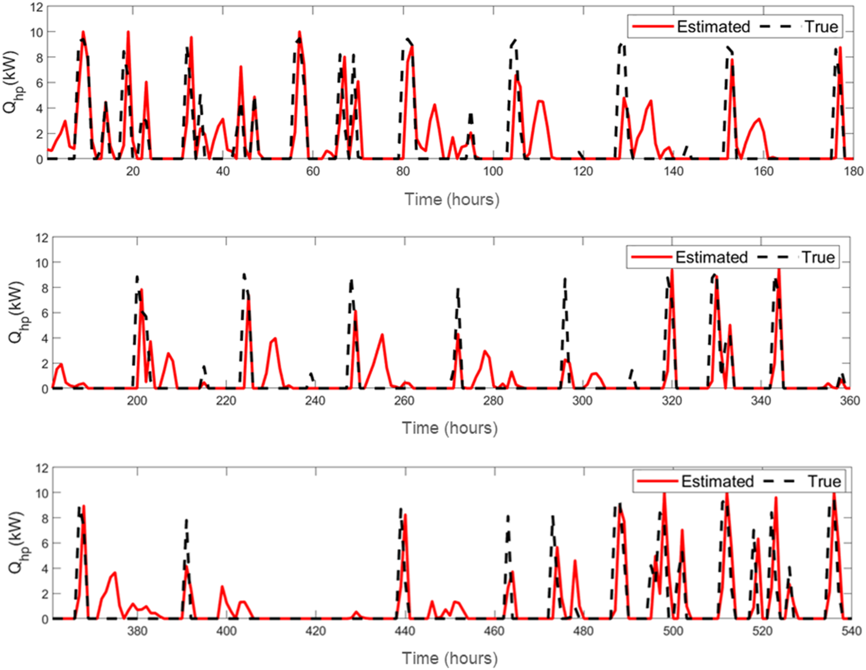
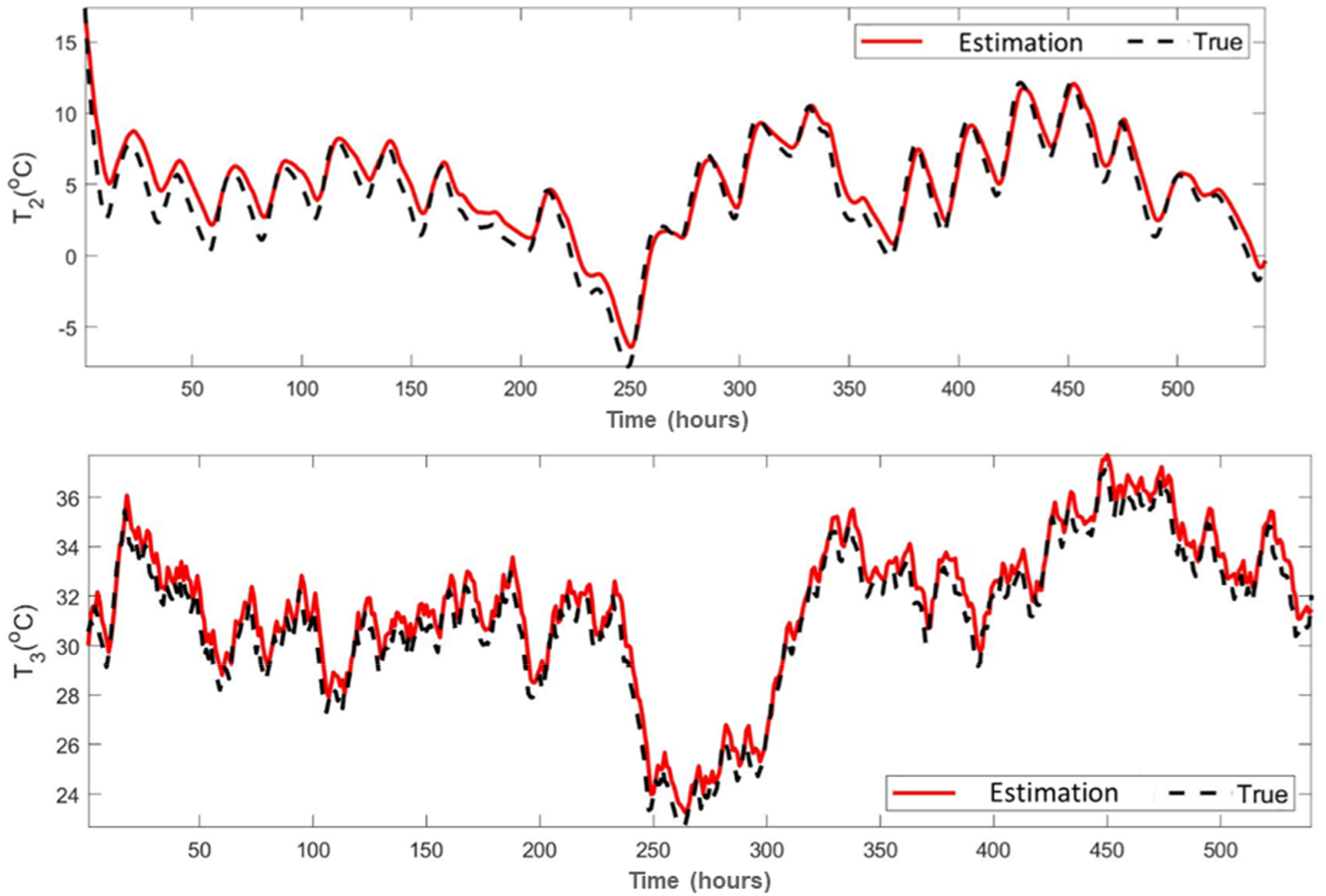
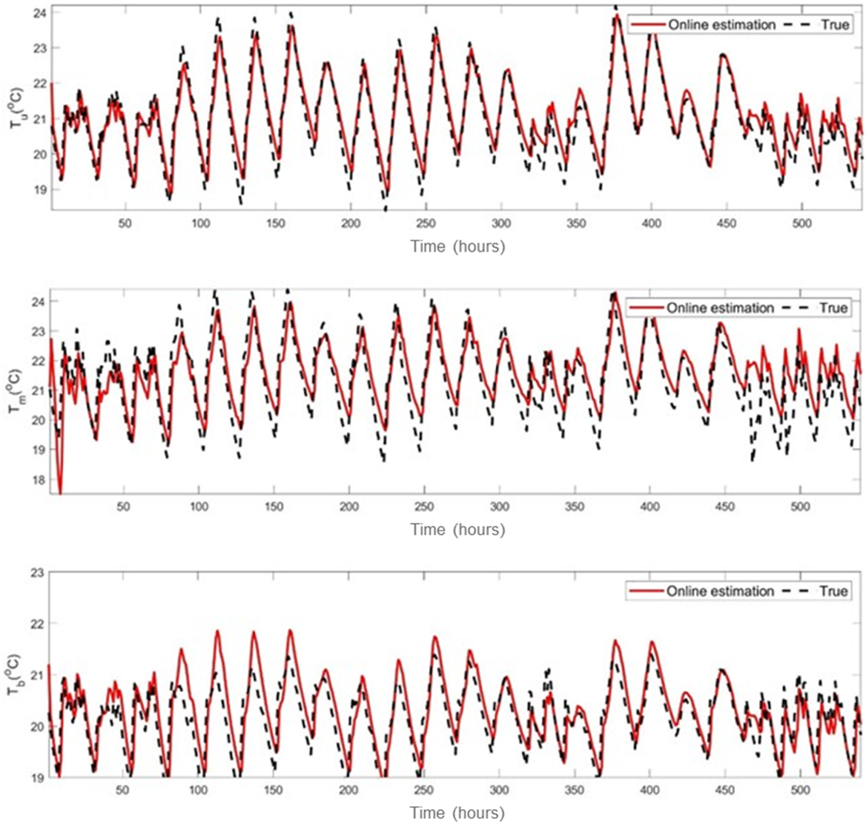
Figure 20 compares the estimated and true temperature response histories for Scenario 10R6C-1. The MAPE of the estimated states (T
u
, T
m
and T
b
) and the corresponding measured (true) values was less than 2% for the three available measurements, indicating a strong agreement between the estimated and the true states. The maximum difference was approximately 1°C. These comparisons demonstrate that the developed method can be effectively applied to real-time temperature prediction for real-world practices. Comparison between true and estimated temperature responses for Scenario 10R6C-1.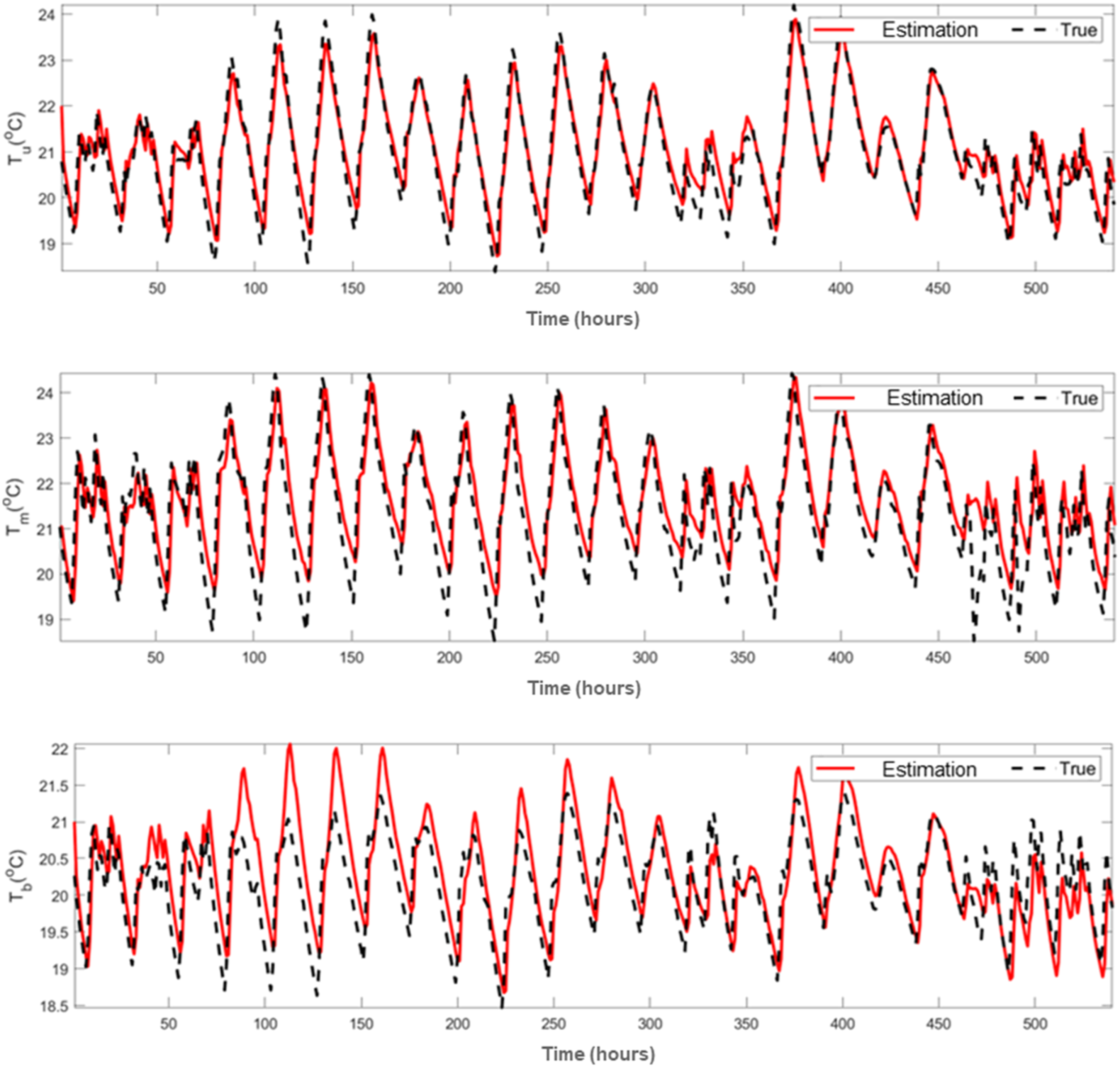
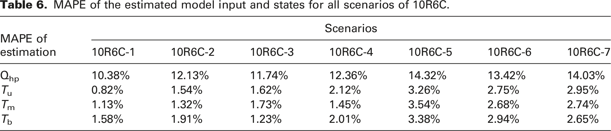
MAPE of the estimated model input and states for all scenarios of 10R6C.
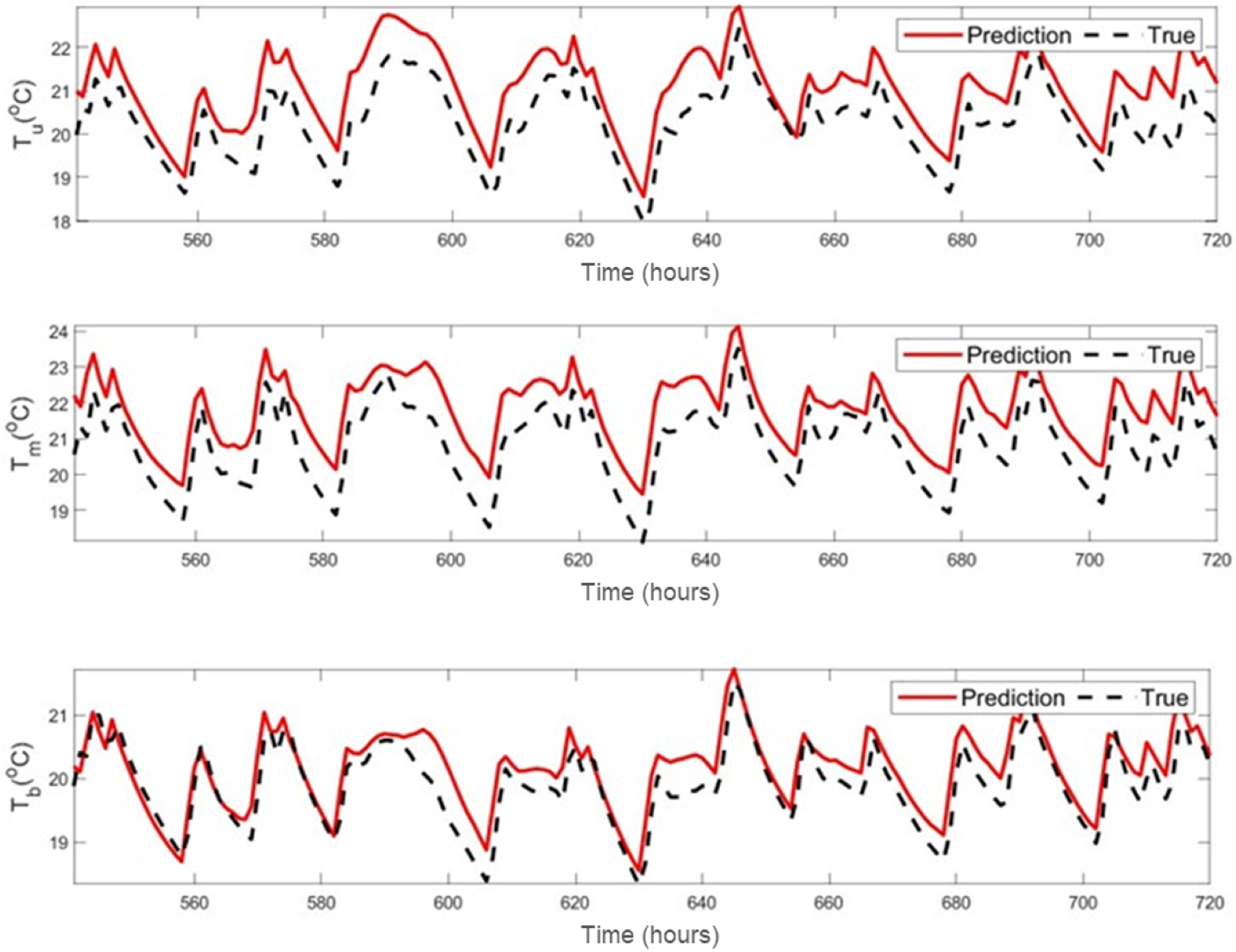
To show the performance of the calibrated RC model for temperature state prediction, Figure 21 compares the measured temperature responses from the prediction dataset to those predicted responses using the parameters obtained at the end of the 540-h estimation period. The RC models were used to simulate the states in the prediction period. Predicted temperature responses were computed at each hourly time step within the hour 541 to 720. The MAPE in the predicted state and measured temperature responses were around 2.5% for each available measurement, indicating that the measured and predicted temperatures are in excellent agreement. This also indicates that the error in estimating the input is acceptable because it does not cause a significant error in the parameter estimation and state prediction. Table 7 presents the MAPEs of the measured temperatures and predicted states based on the final estimated model parameters derived from the estimation dataset for all scenarios. All MAPE values were less than 5.2%. The accurate predictions of future states reflected in Figure 21 and Table 7 indicate that the model parameters were effectively estimated even with a limited number of missing state measurements. Comparison between true and predicted temperature responses for Scenario 10R6C-1. MAPE of the predicted responses for the 10R6C model in different scenarios.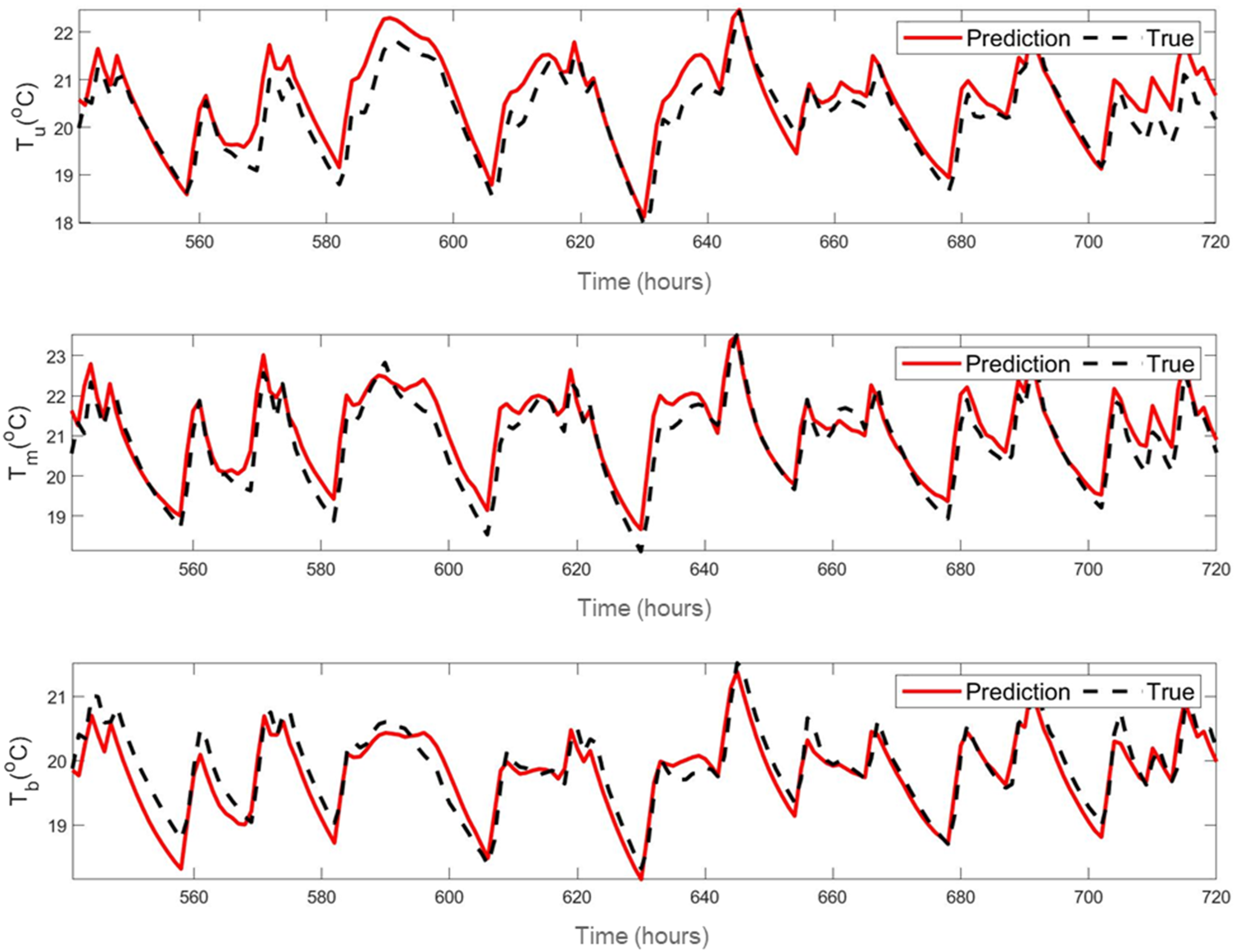
Final estimated parameters in different scenarios for the 10R6C model.
10R6C model parameters estimation: thermal resistances for scenario 10R6C-3.
10R6C model parameters estimation: thermal capacitances for scenario 10R6C-3.
10R6C model parameters estimation: solar and internal gain factors for scenario 10R6C-3.
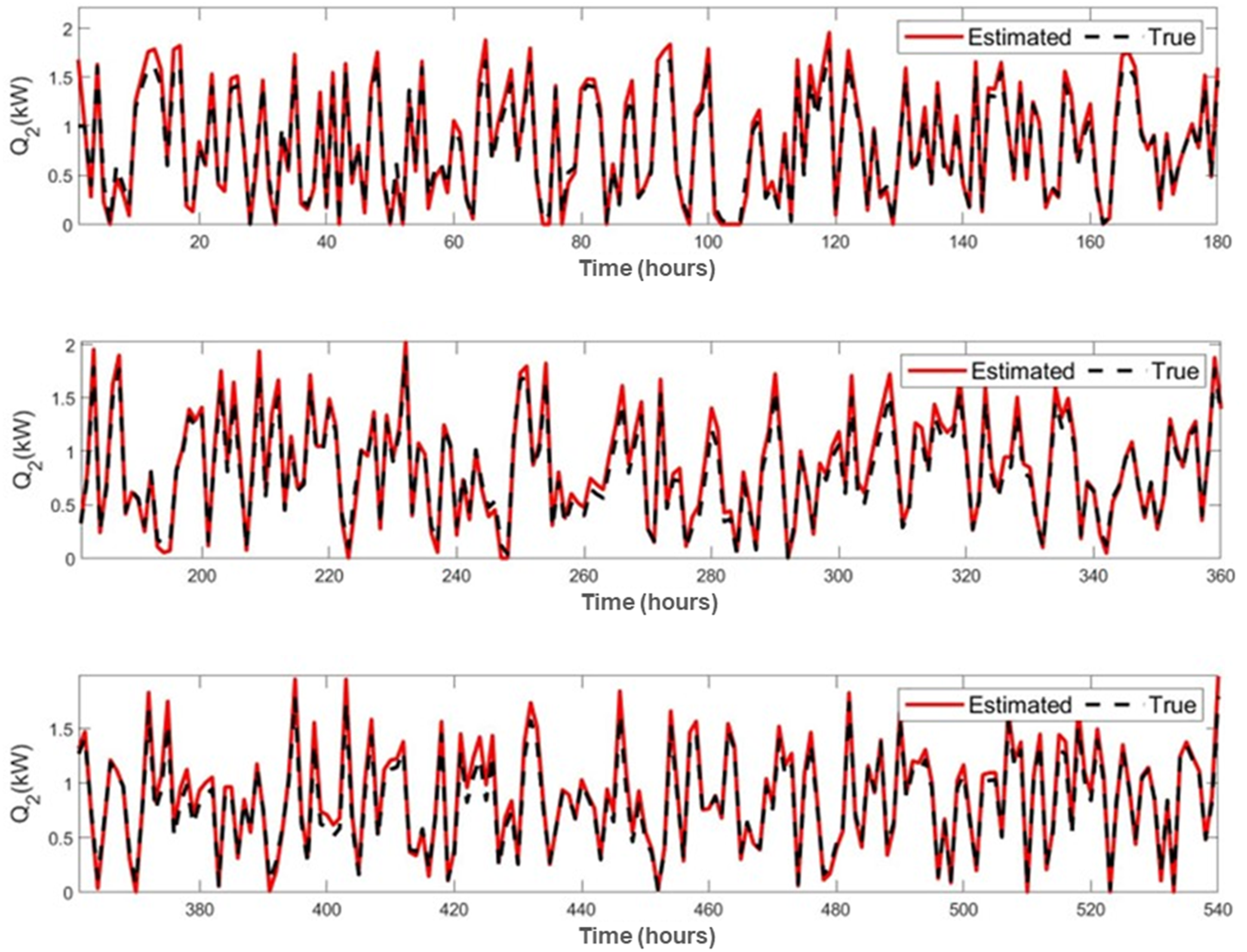
Comparison between true and estimated model input for scenario 10R6C-3.
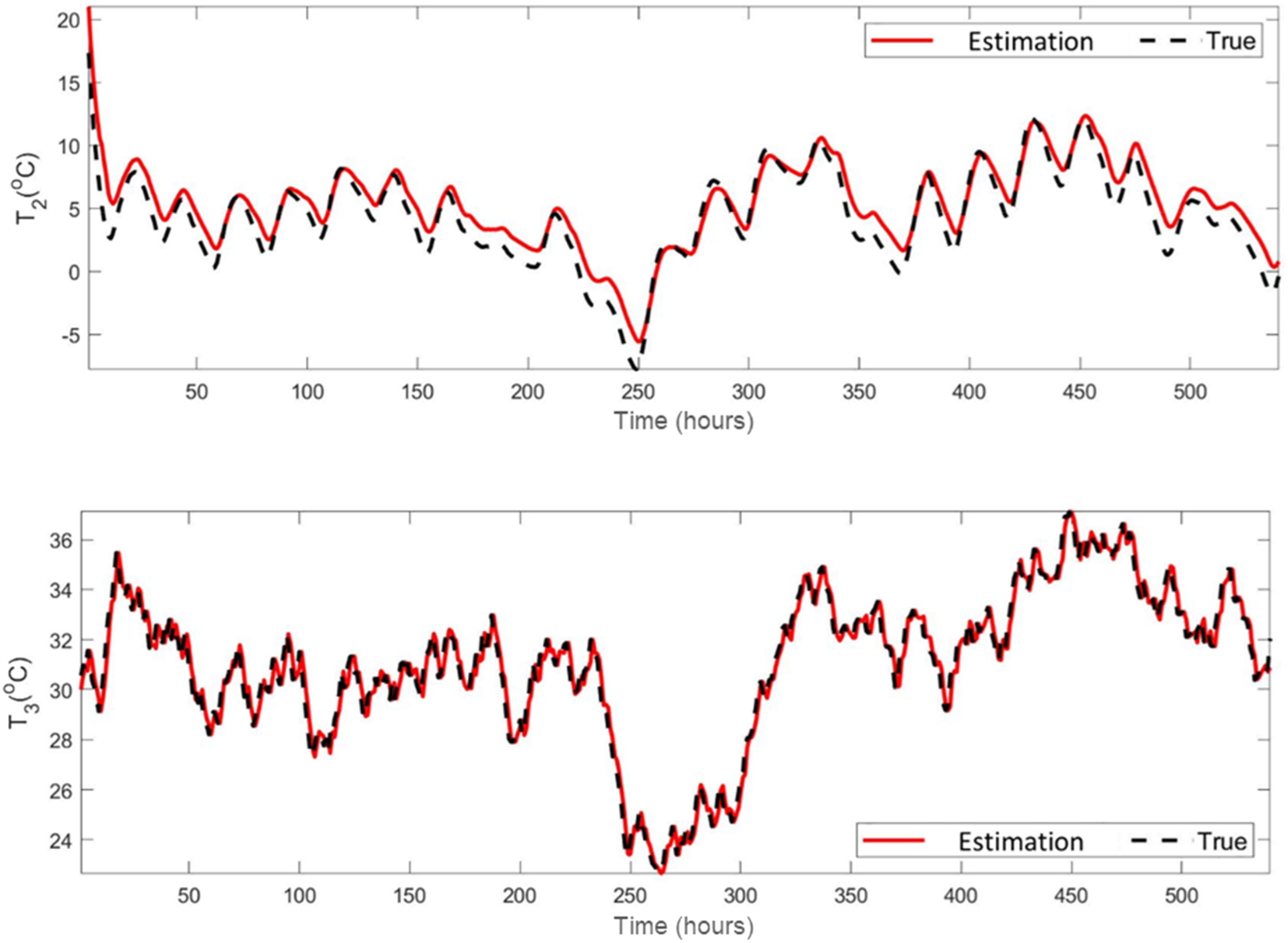
Comparison between true and estimated temperature responses for scenario 10R6C-3.
Comparison between true and predicted temperature responses for scenario 10R6C-3.
Conclusion
Previous research focused on developing methods for model parameter estimation with all model inputs available. This study developed an effective method for estimating RC model parameters and inputs with possible unmeasured temperature states. In this regard, the thermal resistor–capacitor network (RC) was used for thermal dynamic modelling and the unscented Kalman filter (UKF) was integrated with the nonlinear least squares (NLS) method to estimate unknown model parameters and inputs. In order to show the applicability of the developed method, two case studies were conducted: one with made-up data and the other with real-world data. Scenarios with different numbers of available temperature measurements were created to evaluate the capability and performance of the developed method in different circumstances.
The estimated model input and states were compared with their true values. The estimated model inputs in all scenarios of the case study with made-up data have a MAPE (mean absolute percentage error) less than 2.5%, while less than 14.5% in the scenarios of the case study with real-world data. Furthermore, comparing model predictions with the true measurements in all scenarios of both case studies shows a maximum MAPE of approximately 5%. These low MAPE values prove that the developed method can effectively estimate unknown model parameters, input and possible missing states.
Footnotes
Acknowledgements
The authors would like to acknowledge Dr A. K. Athienitis and his research team at Concordia University for providing the data.
Author contributions
Vahid Zamani: conceptualization, developing methodology, analysis implementation and writing the original draft. Shaghayegh Abtahi: Manuscript revisions. Yuxiang Chen: supervision, conceptualization and manuscript revisions. Yong Li: supervision, conceptualization and manuscript revisions.
Declaration of conflicting interests
The author(s) declared no potential conflicts of interest with respect to the research, authorship, and/or publication of this article.
Funding
The author(s) disclosed receipt of the following financial support for the research, authorship, and/or publication of this article: This work was supported by the Natural Sciences and Engineering Research Council of Canada (NSERC) Collaborative Research and Development Grants, CRDPJ 530932-18 entitled ‘Intelligent net-zero energy (ready) modular homes for cold regions’.