
Abstract
Buildings can have varying heating and cooling set points to take advantage of favorable environmental conditions and low time-of-use rates. To optimize temperature scheduling and energy planning, building energy managements need reliable building thermal models and efficient estimation methods to accurately estimate space heating and cooling supply (or power demand) over a certain period (e.g., 24 h). This accurate estimation capability is vital for performing temperature control strategies. Therefore, the present study used resistor-capacitor (RC) models and unscented Kalman filter (UKF) integrated with nonlinear least square (NLS) to develop a method for precisely estimating heating and cooling supply to control zone temperature. To evaluate the capability of the method, two case studies are conducted. The first case study involves a made-up simple RC model, while the second case study uses monitored data from a single detached house in different scenarios. The capability of the method is evaluated by applying the estimated heating and cooling supply to the RC thermal model and simulated zone temperatures. Then, assess whether the controlled zone’s temperature meets the expected temperature or not. The performance evaluation shows that the developed method can accurately estimate the heating and cooling supply, validating its applicability to temperature control objectives.
Practical Application
This research provides a valuable contribution to modern building industry professionals by offering a precise method for estimating heating and cooling supply for temperature control in buildings. By equipping practitioners with an effective tool to optimize energy management, this study addresses a critical aspect of building performance. The practical case studies demonstrate the versatility and applicability of this approach in real-world scenarios. In a world increasingly prioritizing energy efficiency and sustainability, this research empowers professionals to make informed decisions, enhance building performance, and contribute to a greener and more sustainable future, all within a concise and actionable framework.
Keywords
Introduction
Buildings are responsible for consuming approximately 40% of the world’s energy. 1 Hence, it is essential to decrease the energy usage of buildings in order to align with worldwide sustainability objectives. 2 Efforts to decrease buildings’ energy consumption involve development and deployment of building energy management systems equipped with control systems that can effectively optimize the energy usage in buildings. 3 Studies suggest that the utilization of these control systems can lead to a notable reduction of up to 30% in building energy consumption.4,5 Control systems necessitate thermal dynamic models and estimation methods to estimate heating and cooling supply required for temperature control purposes.
Control systems are widely considered a promising algorithm for achieving energy efficiency in smart buildings. 6 These control systems rely on dynamic and simplified building energy models that describe the thermal behavior of buildings. 7 Various modeling strategies, such as “white box,” “black box,” and “gray box” modeling, have been developed in the literature.8,9
White-box modeling, also known as physics-based modeling (e.g., EnergyPlus and TRNSYS), involves describing building dynamics based on construction information and utilizes parameters derived from comprehensive technical documentation, such as architectural design, material properties, and equipment specifications.10,11 While such data can provide detailed insights into building performance, they pose significant challenges, particularly when dealing with existing structures. Obtaining this level of physical information can be a formidable task, often requiring extensive data collection efforts and, in some cases, may not be feasible for older buildings or structures where documentation is lacking. Moreover, a fundamental limitation of white-box models is their inherent static nature. Once constructed, they tend to operate within the confines of the data and model structures provided during their initial setup. This rigidity can be a critical drawback, especially in scenarios where external conditions are subject to continuous change, such as fluctuations in outdoor temperatures or evolving occupant behavior. White-box models are less adept at adapting to real-time data updates, thus limiting their utility in dynamically changing environments. As a result, applying white-box models in control systems can be challenging.12,13 Conversely, black-box modeling employs pure mathematical machine-learning techniques, such as Artificial Neural Networks, to establish relationships between input and output data without relying on explicit physics-based knowledge.14,15 This modeling approach can offer higher precision than white-box modeling but demands a substantial amount of data to build an accurate model.12,16 However, employing black-box modeling in control systems can be difficult due to its data-intensive nature, potential lack of interpretability. 17
Gray box modeling, such as thermal resistor-capacitor network (RC), is rooted in a physics-based structure and utilizes mathematical optimization techniques to estimate the model’s equivalent physical parameters. 18 This approach combines the advantages of both white-box modeling to eliminate outliers and black-box modeling to reduce the need for detailed information. 18 By striking a well-balanced compromise between interpretability and accuracy, gray box models prove highly suitable for integration into control systems. 19 RC models are based on a set of equivalent model parameters, resistors (R’s) representing thermal resistors. These are similar to the resistance to heat flow that various building components, such as walls, roofs, or windows, offer. Higher resistance values signify slower heat transfer, which might be the case in well-insulated walls, for example. On the other hand, lower resistance values indicate faster heat transfer, as in the case of a window that is not well-insulated, and capacitors (C's), representing thermal capacitors, which stand for the thermal energy storage capacity of a node or component. The ‘C’ value is associated with how much thermal energy a component can store and release. Components with higher ‘C’ values can absorb and store more heat, resulting in slower temperature changes, while lower ‘C’ values respond quickly to heat fluctuations, resulting in rapid temperature changes. This illustrates how much thermal energy can be stored and released in these nodes. These model parameters relate system inputs (e.g., heating and cooling supply) and temperature states. The gray-box modeling approach has been widely used for thermal dynamic modeling.18–20 To develop a reliable control system besides having a reliable thermal dynamic model, a dependable estimation technique is required that can be integrated with RC models to accurately estimate behavior of building systems, particularly for estimating heating and cooling supply (i.e., RC model input).
The successful implementation of building’s control systems relies on the precise controlling of future building’s temperature states with estimation of building systems behavior (i.e., heating and cooling supply). This is because these estimations directly impact the building’s performance and energy efficiency. 19 For instance, in heating, ventilation, and air conditioning systems, inaccurate estimation of supply can cause excessive heating or cooling supply, resulting in increased energy consumption, and operating costs. Such inaccuracies in estimation of building systems behavior (i.e., heating and cooling supply) can significantly affect overall building performance. 21 Therefore, reliable estimation methods should be integrated as part of control systems in addition to thermal models. One such method is Unscented Kalman filter (UKF) which is widely used in estimation problems.22,23 As a result, this paper aims to develop an approach for buildings control applications that utilizes the UKF-based estimation technique in combination with RC models to estimate the heating and cooling supply (or power demand) over a certain period (e.g., 24 h)., for controlling the temperature of thermal zones.
In terms of paper organization, following introduction, this paper presents a method for combining thermal dynamic models with an estimation method for control systems. This involves a description of the RC models used for thermal dynamic modeling, as well as the UKF integrated by the Nonlinear Least-Square (NLS) as an estimation method. Additionally, in the section on application examples, two examples will be provided to demonstrate the use of the developed method: The first example will use a made-up simple RC model (made-up parameters and inputs, and states simulated using the model), while the second example will use a complex RC model with real-life data. These examples will test the capability of the developed method in estimating heating and cooling supply for temperature control purposes.
Problem statement and methodology
Controlling temperature in thermal zones can present significant challenges, particularly when estimating and planning the heating and cooling supply. This challenge becomes even more pronounced when dealing with multiple interconnected zones, each with varying temperatures, as it requires estimating the temperature of uncontrolled zones within the network. To ensure a precise estimation of the required supply for a specific zone, it is crucial to consider the temperatures of other interconnected zones. To achieve this, a method as shown in Figure 1 is developed to estimate the necessary mechanical supply (i.e., RC model input), based on the expected temperature set points. The developed method utilizes a RC thermal dynamic model to represent a thermal system such as one or multiple thermal zones. Notably, the optimal efficiency of this method becomes evident in existing buildings, where it harnesses historical data to construct the RC thermal dynamic model, subsequently replacing the newly developed approach with an established controlling method. Furthermore, it can be used for new buildings with similar design and energy systems. General procedure of mechanical supply estimation to control temperature.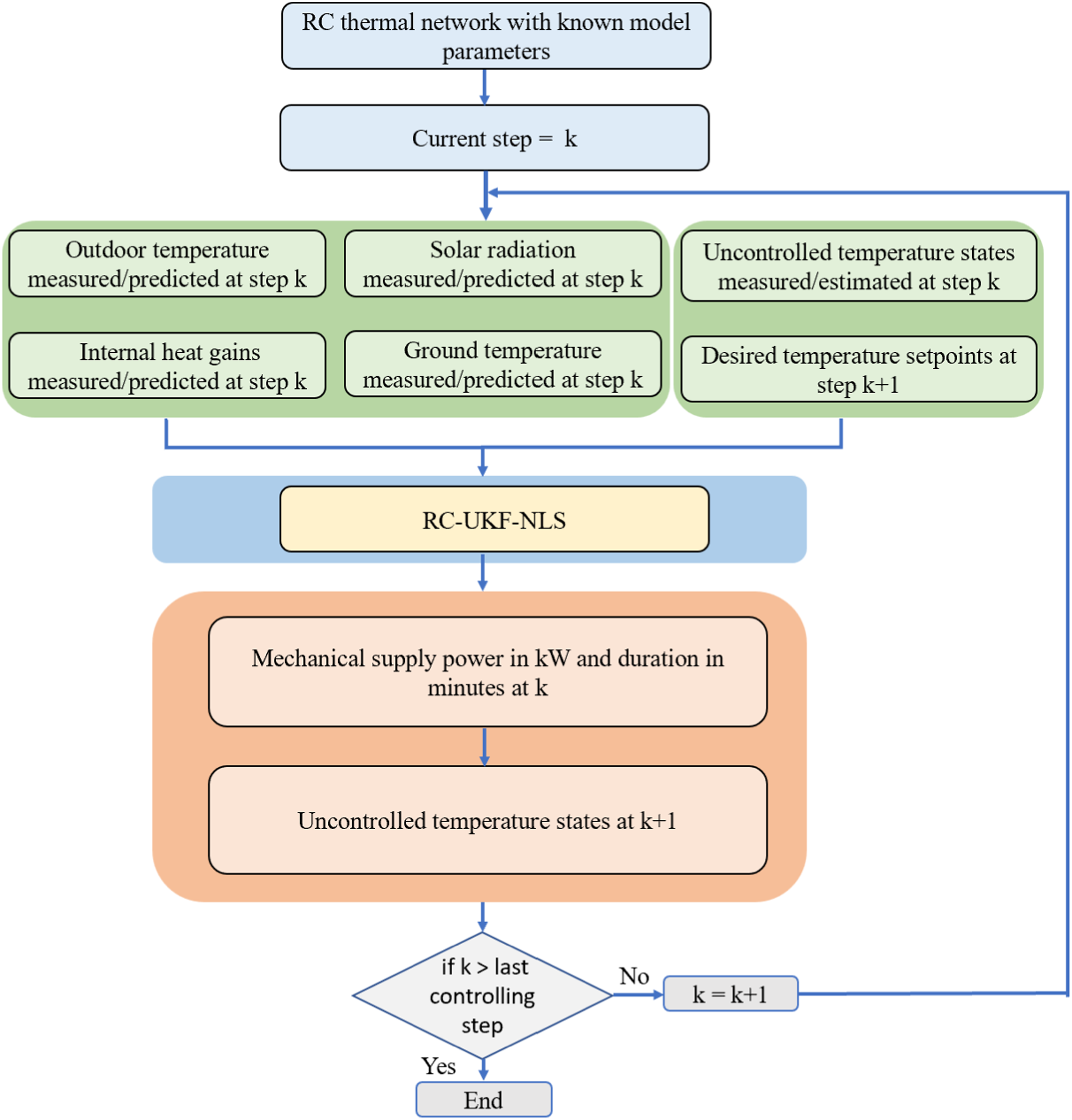
To estimate the required mechanical supply of a thermal system represented by an RC thermal model, several additional variables need to be considered. These include the uncontrolled zone temperature which is measured for the current step and estimated for the rest, as well as the temperature set point, which needs to be defined based on the desired temperature level. Additionally, other boundary conditions, such as outdoor temperature and solar irradiation, must be considered. These boundary conditions are measured for the current time and predicted for the rest of the controlling dataset. Accordingly, the method involves the use of RC models and UKF and NLS estimation methods to estimate the necessary mechanical supply for controlling the temperature of different zones.
In this section, thermal dynamic modeling employing RC models will be discussed, followed by the estimation method based on the integration of the UKF and NLS. The UKF is used to estimate the temperatures of the uncontrolled zones, while the NLS is employed to estimate the required heating and cooling supply. It is worth noting that this method operates recursively, allowing it to update itself with new measurements and estimate the heating and cooling supply based on recent data. This adaptive capability enables the tool to adjust to new information, such as outdoor temperature or solar irradiance, occupant behavior, and window openings, this adaptability is a key strength of the model, as it enables to calculate the necessary adjustments to maintain the desired temperature in the designated zones. As such, this tool can continuously monitor and update its estimates to ensure optimal performance and energy efficiency.
Thermal dynamic modeling using RC models
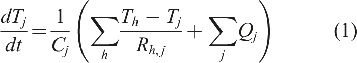
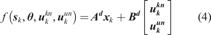
In modeling the thermal dynamics of a building, the RC model is utilized to represent temperature nodes within the building’s thermal zones. Each temperature node is connected to model parameters (represented by R’s and C’s) and inputs (such as solar heat gain or mechanical heating/cooling supply). These interconnected model nodes form an RC thermal model, where the connections between nodes are represented by R’s. The parameters, inputs, and model nodes together create a thermal RC model. Running the RC model with inputs (i.e., simulation) will provide temperatures at the model nodes (i.e., states). The thermal dynamics at each node can be presented by ordinary differential equations (ODEs). The typical equation for a node, say

Model input estimation method
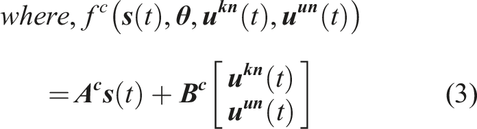
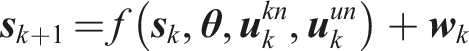
This section describes the method for estimating unknown model inputs, and uncontrolled temperature states, using the UKF integrated with NLS. Equation (2) can be written as a continues nonlinear state equation in the presence of additive process noise shown in equation (3):

In the estimation method, measurements of thermal dynamic model responses (i.e., defined set points or controlled zone’s temperature) can be linked to the model prediction through the measurement equation, shown in equation (5):


UKF is a Kalman-based technique that combines a measurement-based correction strategy with a prediction strategy based on unscented transformation (UT). The UT, often used in the context of nonlinear estimation and Bayesian filtering, is a method for propagating the mean and covariance of a probability distribution through a nonlinear function.
29
In the prediction step, UKF utilizes UT to estimate the mean and covariance matrix of a nonlinear function by evaluating a set of deterministically selected points, known as sigma points (SPs). SPs are a set of representative data points strategically selected from a probability distribution, to capture essential distribution characteristics like mean and covariance when estimating nonlinear transformations.
29
The UT requires the selection of
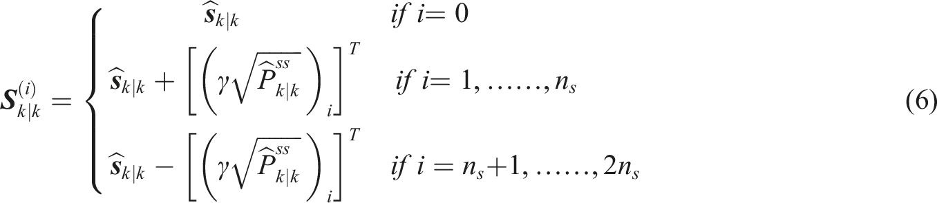
By using the initially determined SPs (i.e.,

With these propagated sigma points, prior estimates of the mean vector and the covariance matrix of the nonlinear state function at time step (k + 1) can be obtained. However, as the state function includes model inputs that need to be estimated, estimation of these inputs becomes a prerequisite for calculating a new set of SPs (i.e.,
In order to estimate heating and cooling supplies (i.e., model inputs), NLS works as an optimization tool to minimize the estimation error. In particular, the estimation error (i.e.,

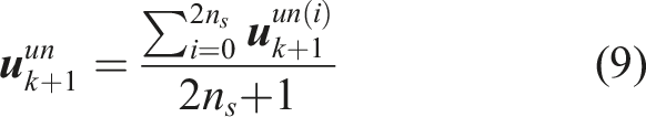
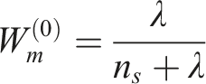
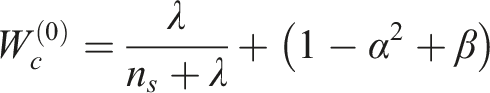
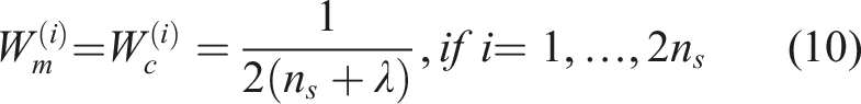
SPs are intended to represent a nonlinear function, which necessitates weighting coefficients to calculate the mean and covariance of the nonlinear function as shown in equations (9) and (10). They categorized as
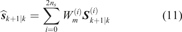
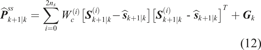
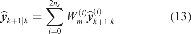
Once the model inputs are estimated and SPs weighting coefficients are determined, the prior estimates for the mean vector
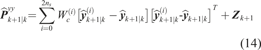
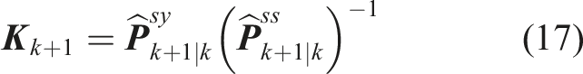
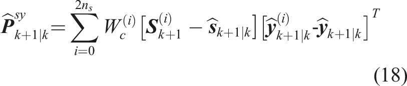
As shown in equations (15) to (18) the correction step is carried out at time step


In summary, Figure 2 shows a flowchart for the developed method that can be used for model input (i.e., heating and cooling supply) and uncontrolled zone’s temperatures estimation that can be employed for controlling zone’s temperature. It is worth noting that implementing these equations manually can pose a challenge for architects or designers; however, they serve as the fundamental basis for the creation of a specialized software tool. Model input estimation method based on UKF integrated with NLS.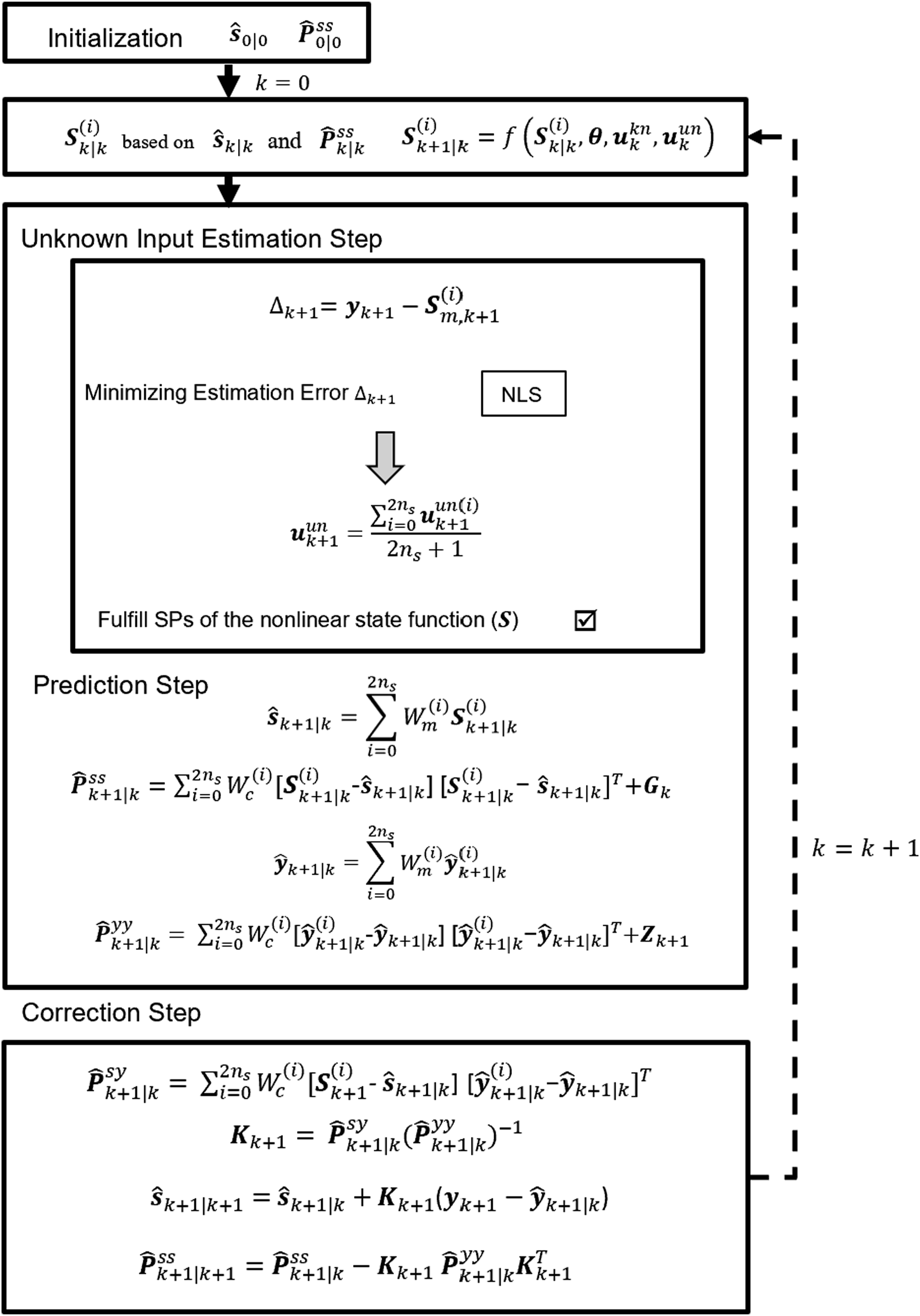
Application examples
Two case studies are presented in this section to illustrate and evaluate the developed method. The first case study uses a simple made-up RC model with two thermal resistances and two thermal capacitances (known as a 2R2C model). The second case study involves a real-world single-family house, which is notably more complex (10R6C). The capability of the developed method in estimating heating and cooling supply (i.e., model inputs) is evaluated by applying the estimated supply and simulating defined RC models to generate the zone temperature and determining whether it is controlled at the desired level or not.
A case study with a made-up RC model
Figure 3 shows the made-up RC model, labelled as 2R2C. This model comprises four parameters, including two thermal resistances (i.e., 2R2C model structure.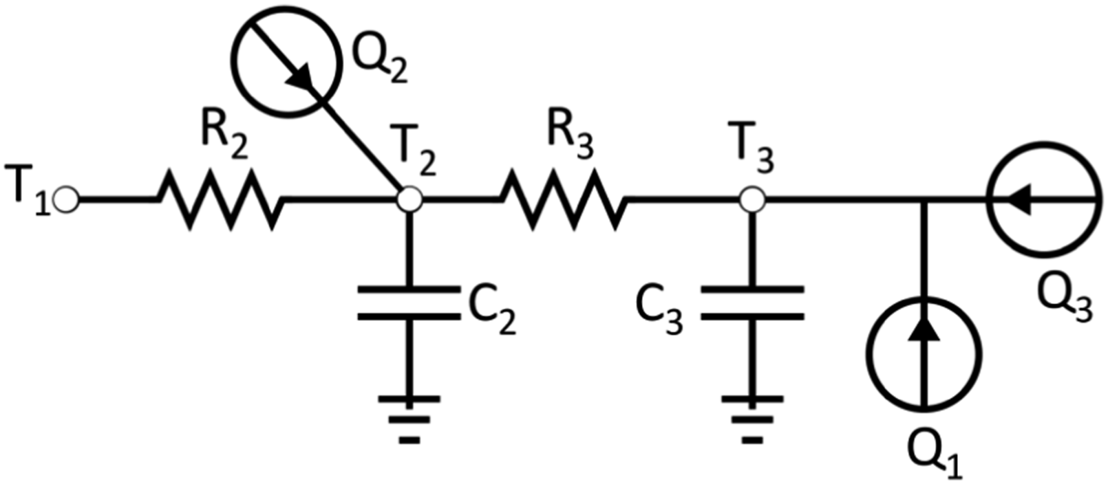
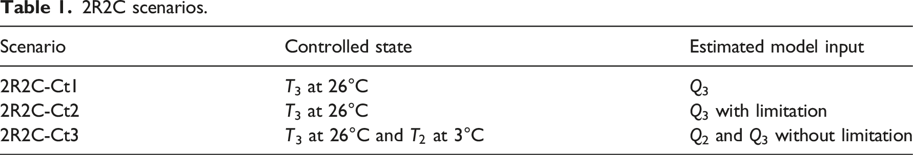
2R2C scenarios.
Assumed model parameters and initial states of the RC model are presented in equation (19). These values are obtained from previous studies.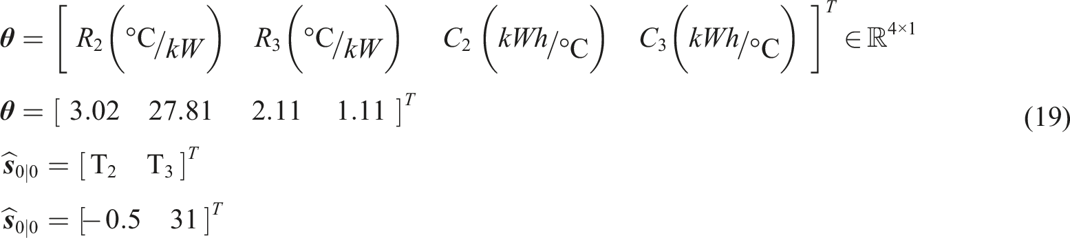
The initial covariance matrix
In Scenario 2R2C-Ct1, in addition to the Q3, the model state (a) Estimated heating and cooling supply, (b) estimated state T2 when T3 controlled at 26°C.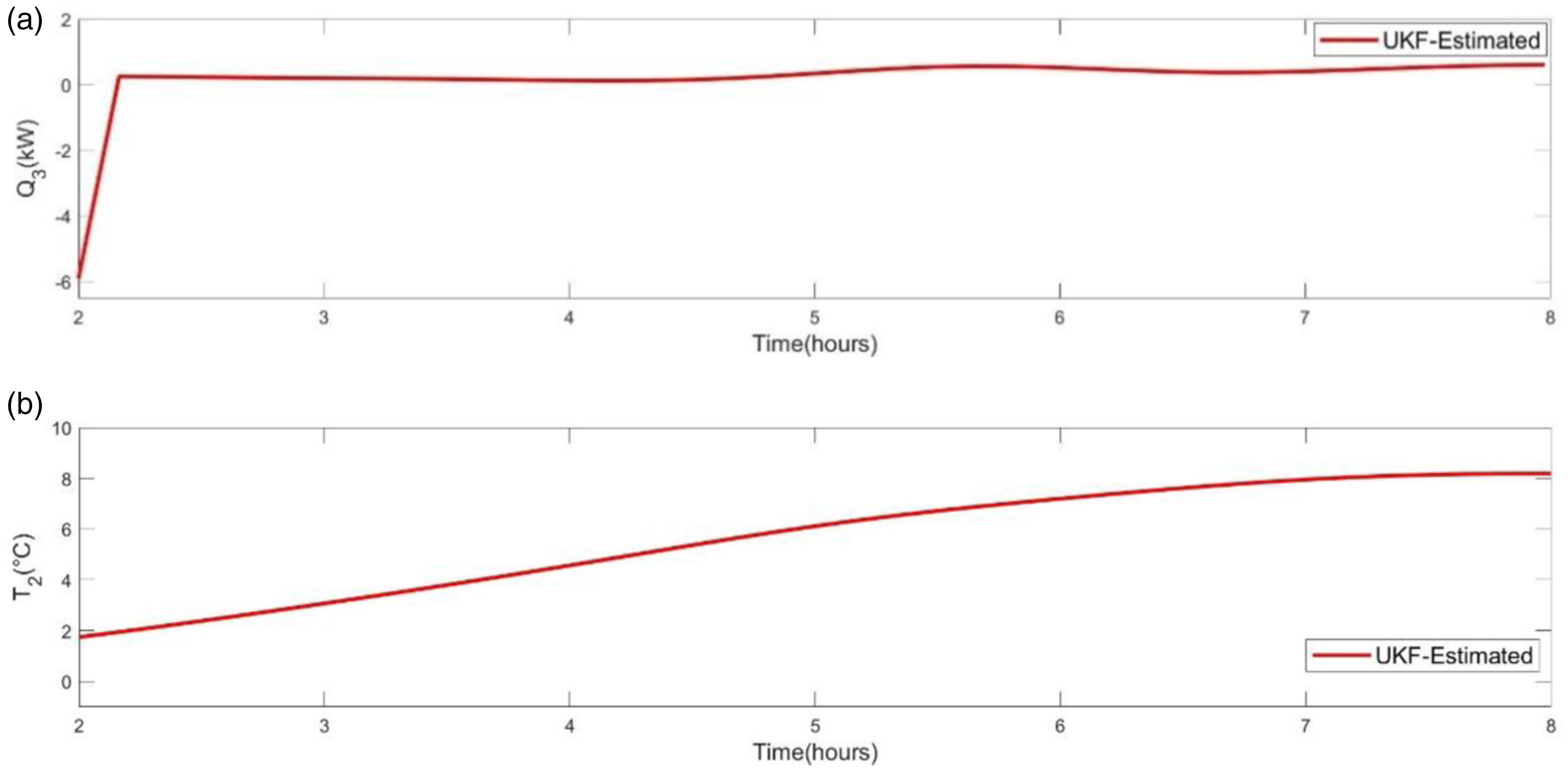
To validate the estimated heating and cooling supply, the estimated Q3 must be taken into account and the previously described 2R2C model simulated in order to generate the system response for T3 and determine whether it is controlled at 26°C or not. Accordingly, Figure 5 depicts the simulation result for T3 in the controlling dataset. The graphs show that T3 falls sharply from 31°C to 26°C in the first 10 min and remains at 26°C for the rest of the controlling period, which starts from hours 2 to 8, it is worth noting that hours 0 to 2 indicate zone temperature T3 behavior prior controlling. This demonstrates that the presented method can accurately estimate the required heating and cooling supply to control T3. T3 in the controlling dataset.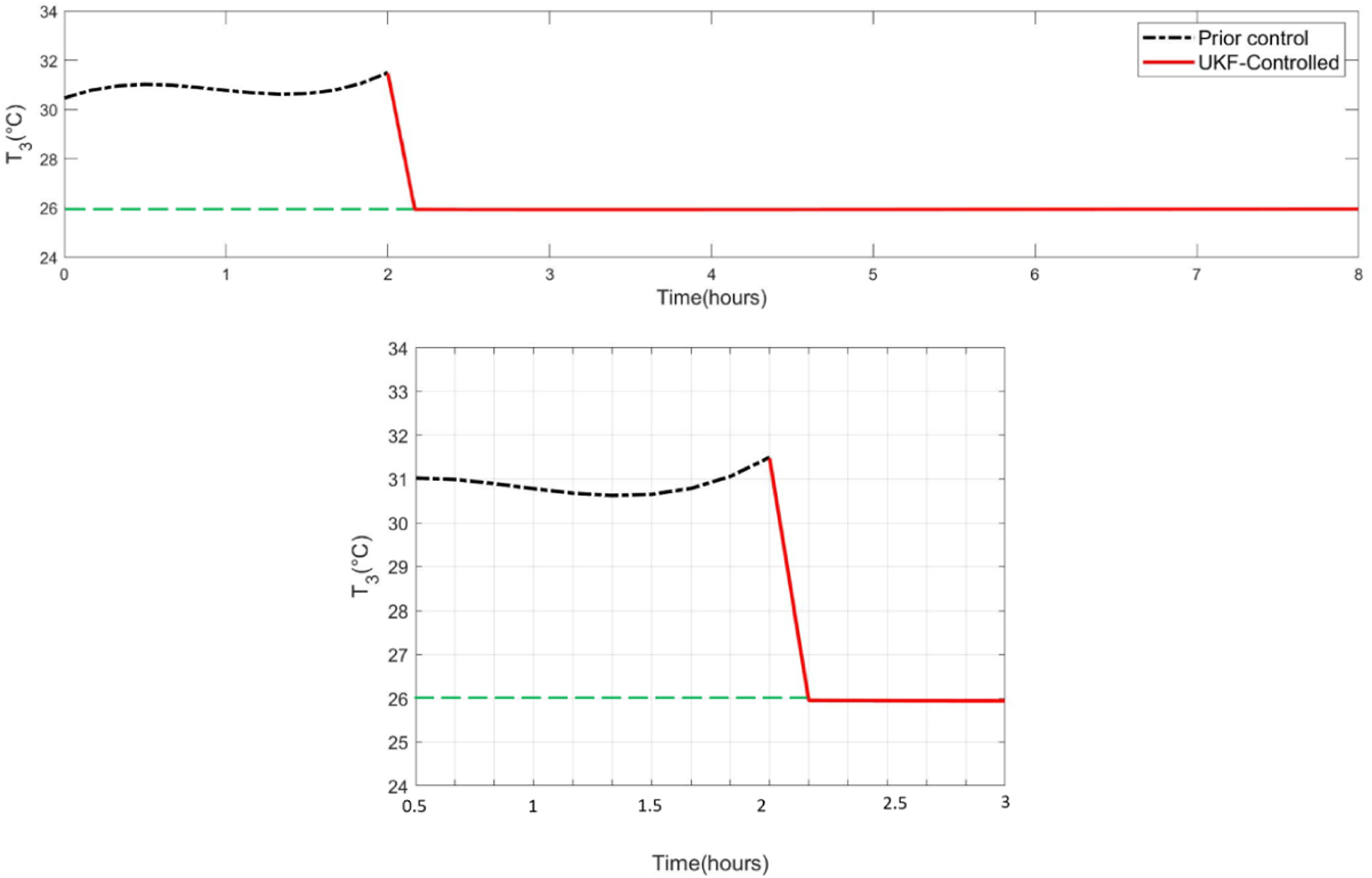
For Scenario 2R2C-Ct2 there is a limitation on the maximum value of the model input, or in other words, equipment with a limited heating and cooling supply capacity. Specifically, the maximum capacity is set at 1 kW. Figure 6 presents the results of this scenario, showing the estimated Q3 in this scenario. To maintain T3 at 26°C and manage the demand for heating and cooling supply, it is essential to sustain the estimated supply at its maximum capacity for an extended period. This is necessary because the required amount of heating and cooling exceeds the capacity of the equipment providing these services. Limited heating cooling supply to 1 kW.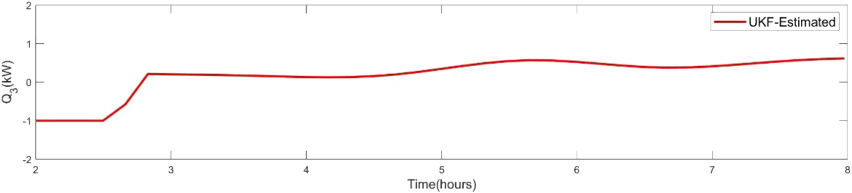
Figure 7 compares the simulated T3 response in two instances, one where Q3 is not limited and the other where Q3 is constrained to a maximum of 1 kW. The first red line corresponds to the scenario in which Q3 is not limited, while the blue line represents the scenario where Q3 is limited to 1 kW. It can be observed that when the estimated Q3 is limited, T3 takes longer to reach 26°C due to the insufficient heating and cooling supply. This highlights the significance of accounting for equipment capacity limitations while estimating the heating and cooling supply and managing building energy. Although the developed method can still estimate the optimal heating and cooling supply required to maintain a constant temperature within the zone, even with limited equipment capacity, it may take more time to achieve the desired temperature. Comparison of T3 for two scenarios 2R2C-Ct1 and 2R2C-Ct2.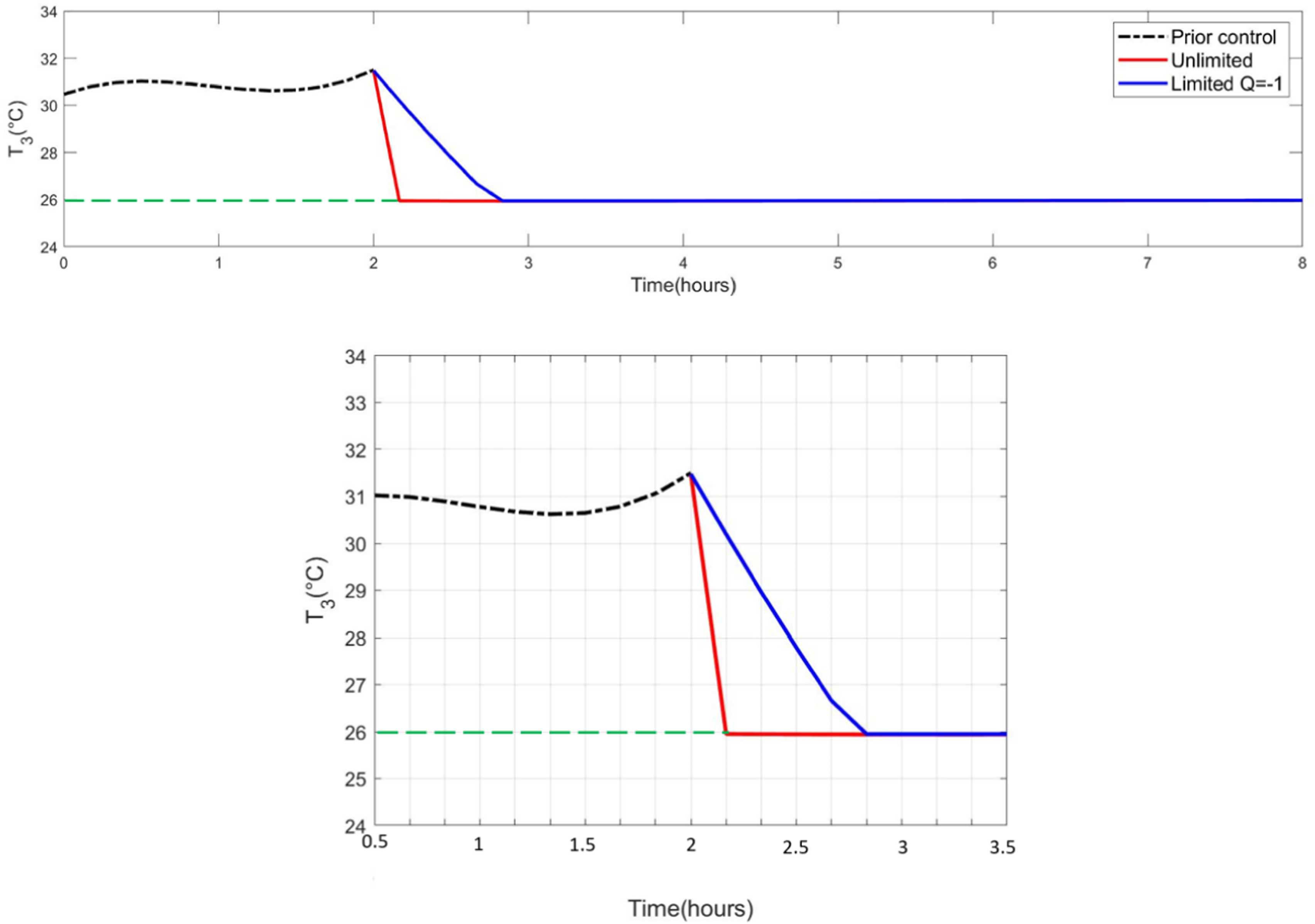
In some situations, it may be necessary to control the temperature of multiple zones simultaneously. In such cases, it is important to estimate the required heating and cooling supply for each zone. For this purpose, Scenario 2R2C-Ct3 is defined, which the objective of this scenario is to control T3 and T2 at 26°C and 3°C respectively, while determining the corresponding heating and cooling supplies needed to sustain these zones at their expected temperatures.
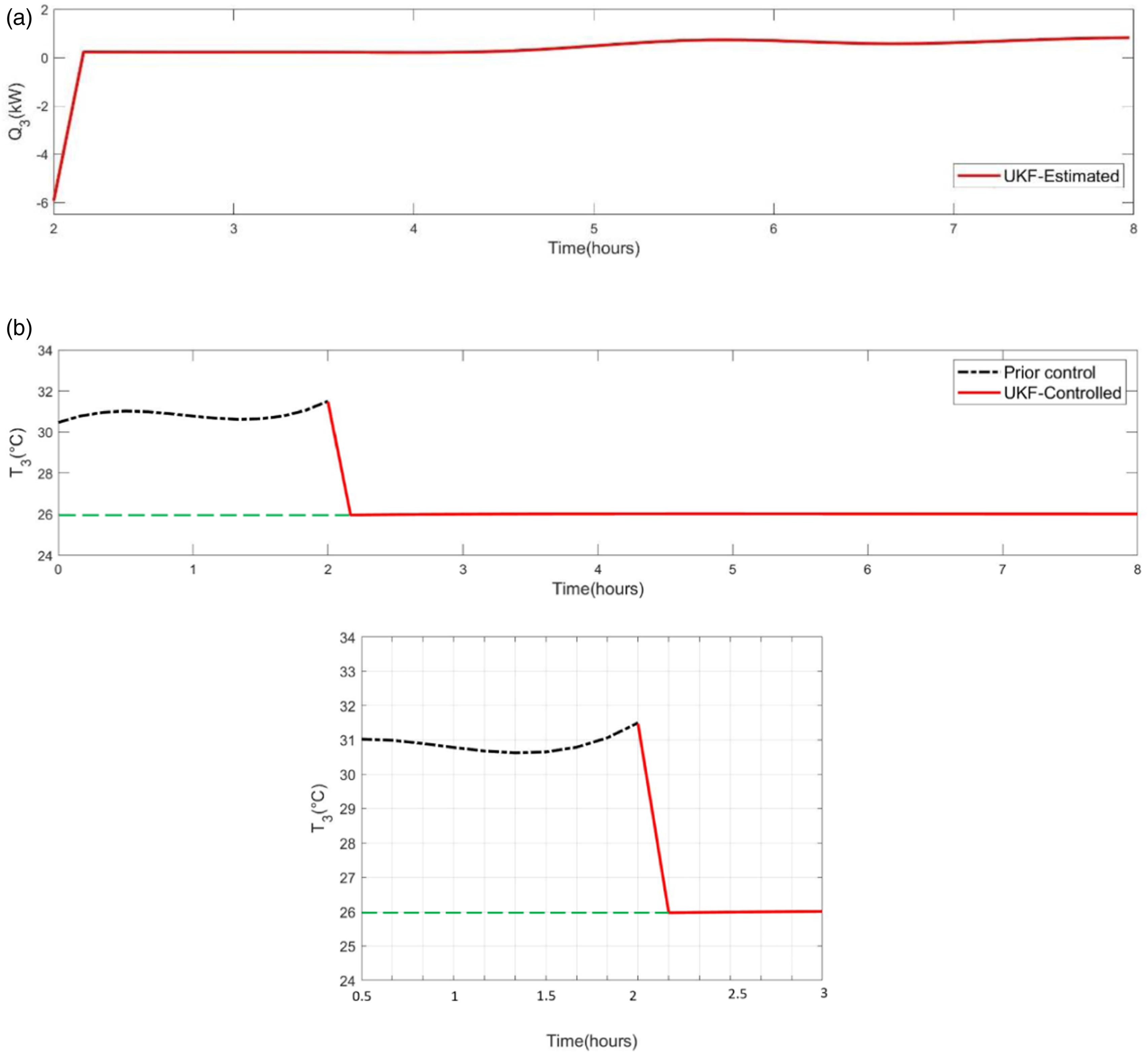
The estimated heating and cooling supply (Q2) required to control node T2 at 3°C is illustrated in Figure 8(a). The estimated Q2 initially amounts to 7.8 kW and varies between 0 and −2 kW (negative, meaning cooling) to maintain T3 at 26°C. Figure 8(b) depicts sharp increase in T2 from about 0°C to 3°C within the first 10 min, after which it remains constant for the control period. Additionally, Figure 9(a) depicts the estimated heating and cooling supply required to control T3 at 26°C. The initial Q3 is −5.5 kW and varies between 0 and 1 kW to maintain T3 at 26°C. Figure 9(b) displays the simulation results for T3 in the control dataset. It is observed that T3 drops quickly from 31°C to 26°C within the first 10 min and stays at 26°C for the remainder of the control period. It is worth noting that the precision of the simulated results, lacking notable oscillations in the model’s temperature response, can be attributed to a combination of factors such as model simplification, high data resolution, and the comprehensive level of detail encompassed by the RC model. Despite serving as a valuable tool for comprehending building thermal behavior, it is crucial to acknowledge that the intricacies of real-world systems may introduce more intricate and dynamic temperature fluctuations that simplified models may not entirely encompass. (a) Estimated heating and cooling supply Q2, (b) T2 in controlling dataset. (a) Estimated heating and cooling supply Q
3
, (b) T
3
in controlling dataset.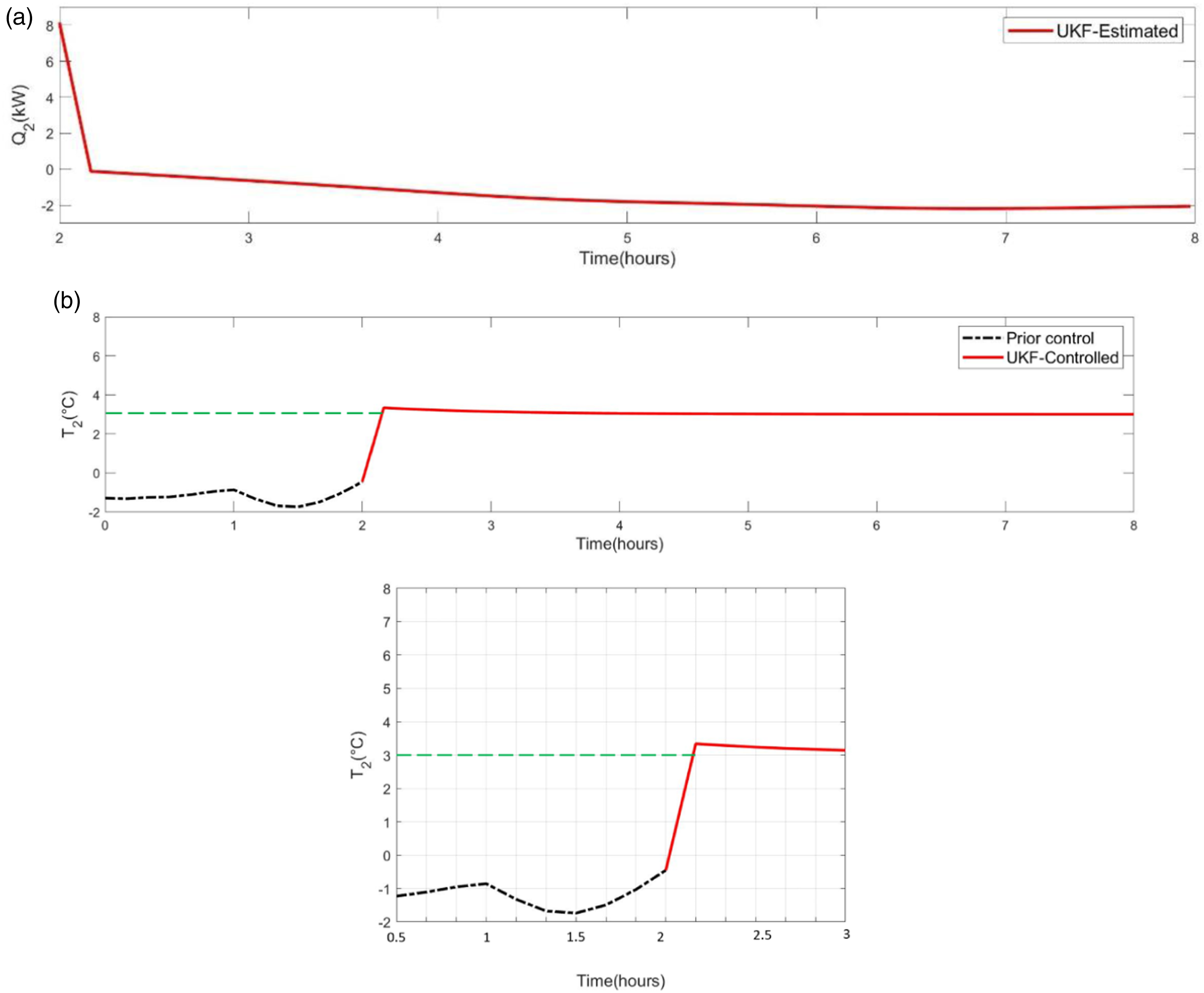
A case study with real-world house
In this section, the developed method is tested on a real-world low-energy wooden-frame house in Eastman, Quebec, Canada, shown in Figure 10. The RC thermal model structure for this house, shown Figure 11, and was developed by Wang et al.
34
This RC model is used for heating and cooling supply estimation for controlling the temperature of different zones of this house for a period of 6 h at 10-min intervals (control dataset). Two scenarios are defined based on controlling different zones temperatures. Accordingly, the capability of the developed method is evaluated by applying the estimated supplies and simulating the RC model to generate the zone temperature and determining whether they are controlled at the desired level or not. Furthermore, it is essential to highlight that the devised method signifies a novel and innovative approach to temperature control in buildings. The present example serves as a tangible demonstration of how this method can be applied effectively to real-world structures, offering an initial practical showcase of its efficacy. Such case studies are often crucial first steps in validating and showcasing the potential of new approaches, paving the way for future research and real-world implementations. A single detached house as a case study.
34
Single-detached house RC model.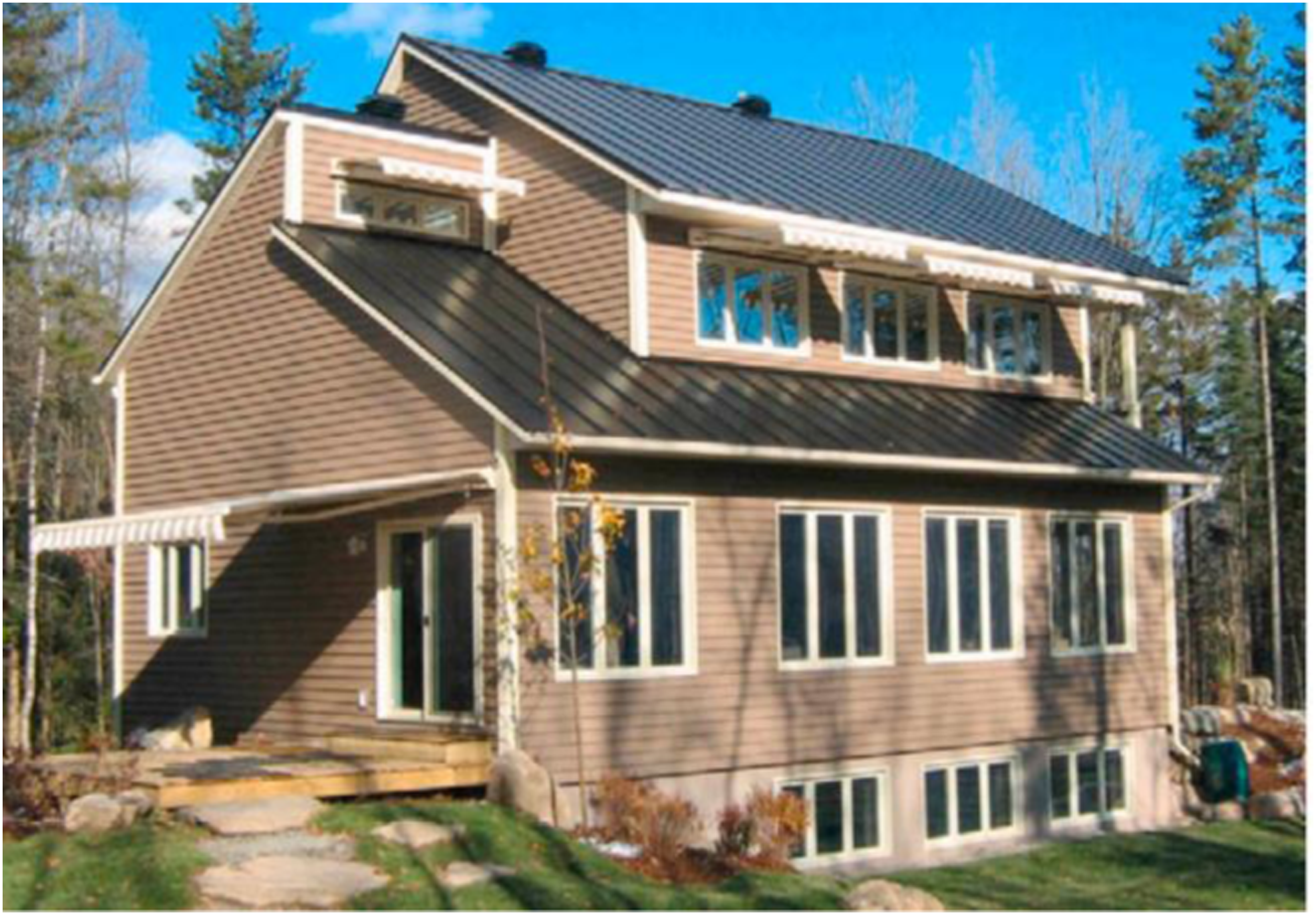
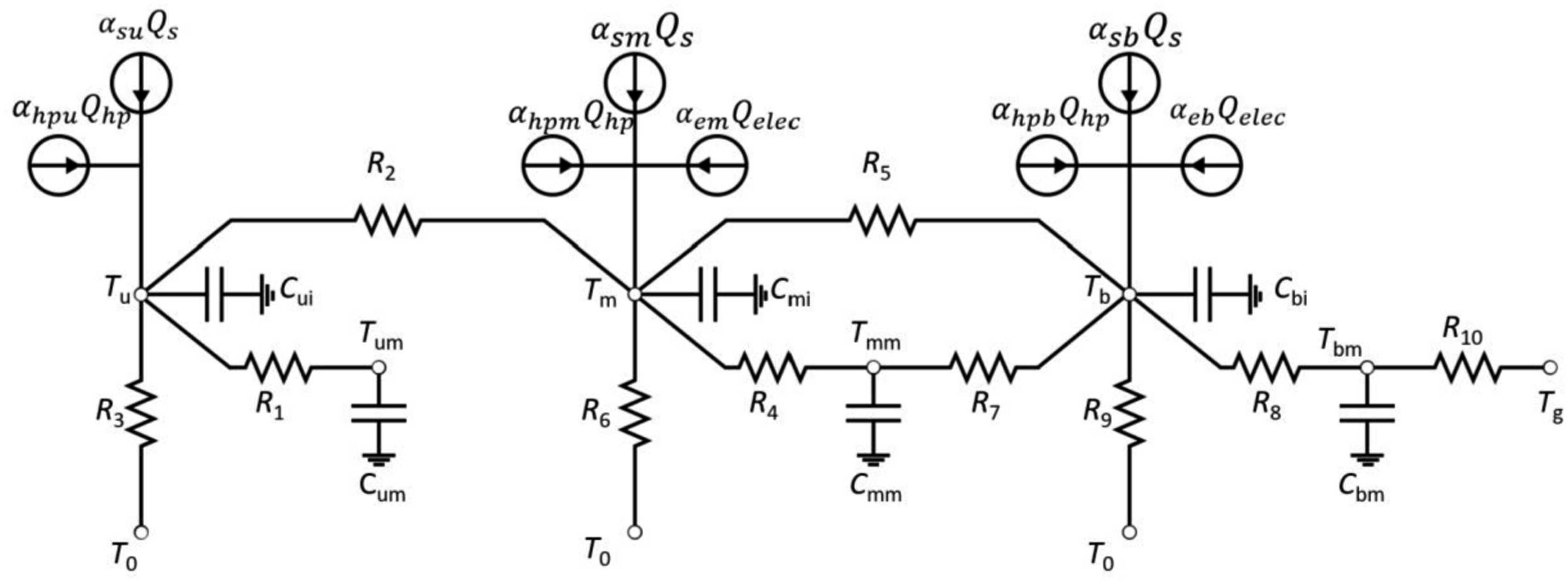
This RC model is called a 10R6C, as it consists of 10 thermal resistances and six thermal capacitances corresponding to six temperature nodes, indicated by T u , T m , and T b in °C for the temperature responses of the second floor, main floor, and basement, respectively. Note that T um , T mm , and T bm are the auxiliary internal temperature responses. The ODEs of this RC model are shown in Appendix B.
The 10-min model inputs for this RC thermal model in the controlling dataset (6 h including hours 2 to 8) are shown in Appendix B. These inputs include (1) global irradiation Q
s
in kW per unit area on the south façade, which is used to obtain approximate effective solar heat gains and is weighted by solar gain factors (α
s
). (2) T
g
ground temperature, which is approximately at 13 C° constants as shown by measurements. (3) T
0
outdoor temperature in C°. (4) Q
elec
gross electricity demand in kW and used to calculate internal heat gains and are weighted according to internal gain factors (α
e
). (5) Q
hp
in kW is the heating supply from the geothermal heat pump, which needs to be estimated in order to control the main floor temperature. (6) Q
hp
is distributed using the alpha distribution factor (
The control system in the house is a normal thermostat. The heat pump runs on an on-off manner. 35 In such a system, the heat pump regulates heating and cooling based on temperature set points and the building’s heating and cooling demand. To implement the newly developed control method, several key steps must be taken. First, the RC thermal model ness to be created and it’s model parameters must be calibrated based on the specific building’s characteristics, ensuring an accurate representation of its thermal behavior. Next, sensors monitoring indoor and outdoor conditions are integrated to provide real-time data to the model. The control system utilizes the RC thermal model, combined with the UKF and NLS methods, to predict the building’s thermal response to heating and cooling. This predictive capability enables continuous adjustments to the supply, optimizing both comfort and energy efficiency.
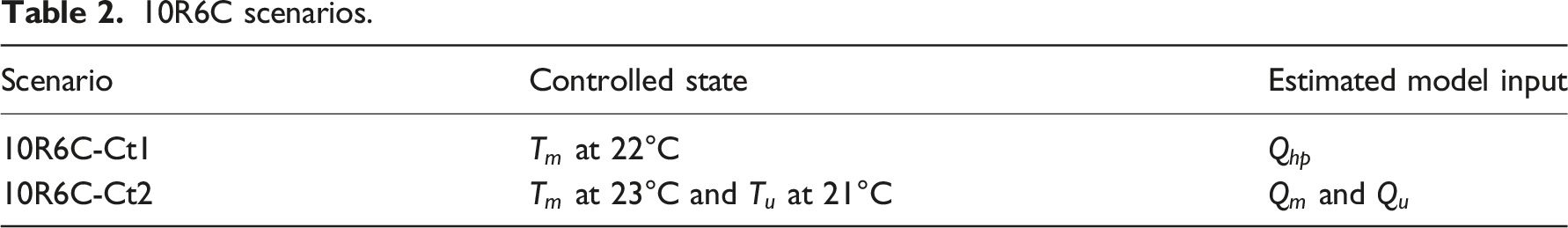
The state vector of this RC model can be defined by Thermal model for controlling two zones’ temperature. 10R6C scenarios.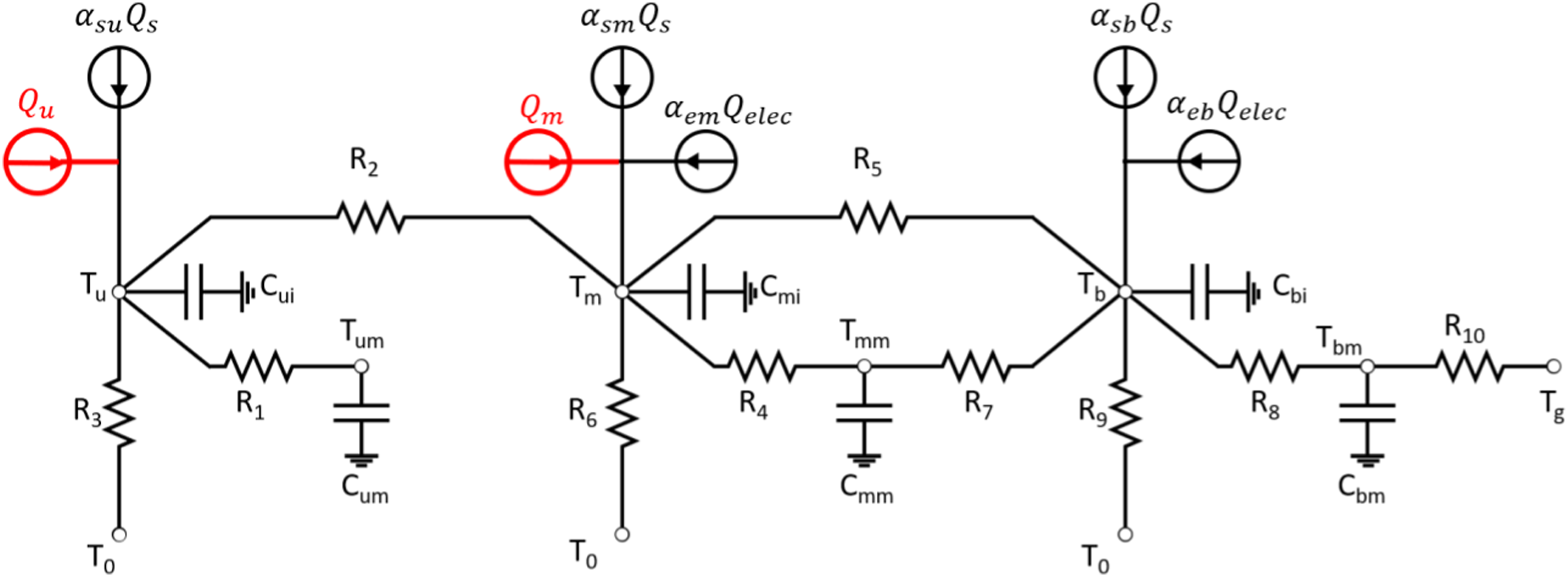
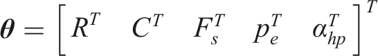
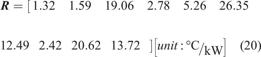
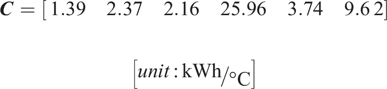
The assumed model parameters and initial states of the RC model is presented in equation (20) and are gotten from the previous studies.


As explained in the case study of a simple RC model, the initial covariance matrix
In Scenario 10R6C-Ct1, the developed method employed to estimate the heating cooling supply Q hp to maintain the main floor temperature Tm at 22°C. Furthermore, Tu and Tb representing second floor and basement temperature will also be estimated during the expected controlling dataset. It is important to note that the maximum capacity of the heat pump installed in this house is 10.55 kW, so the estimated Q hp cannot exceed this value.
Figure 13(a) shows the estimated Q
hp
and uncontrolled state (Tu and Tb) for the controlling dataset. The estimated Q
hp
starts with an initial value of 5 kW and then mostly varies between 0 and 4 kW to maintain Tm at 22°C. Figure 13(b) displays the estimated temperature for the second floor and basemen which are around 21°C and 20.5°C, respectively, when temperature of the main floor is controlled. (a) Estimated heating and cooling supply. (b) Second floor and basement estimated temperature when Tm controlled.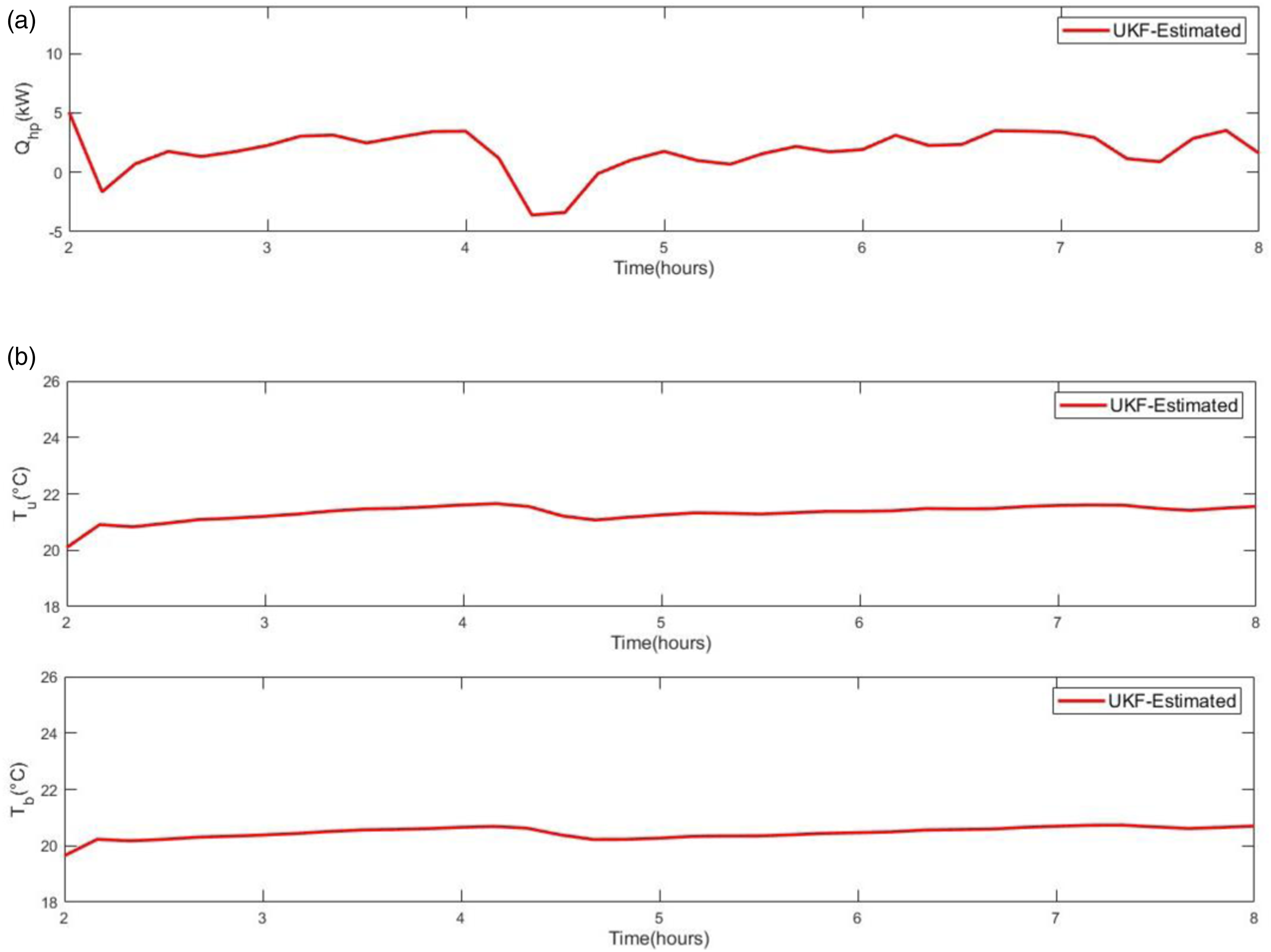
To validate the estimated heating and cooling supply, the estimated Qhp is taken into account and the previously described 10R6C model is simulated to check if the temperature Tm is controlled at 22°C or not. Figure 14 shows the simulation result for Tm in the controlling dataset. It can be observed that Tm increases rapidly from around 21°C to 22°C in the first 10 min and remains at 22°C for the remainder of the controlling period which starts from hours 2 to 8, it is worth noting that hours 0 to 2 indicates zone temperature Tm behavior prior controlling. This indicates that the presented method can accurately estimate the required heating and cooling supply to control the temperature of the main floor Tm. Results for Tm the controlled data set.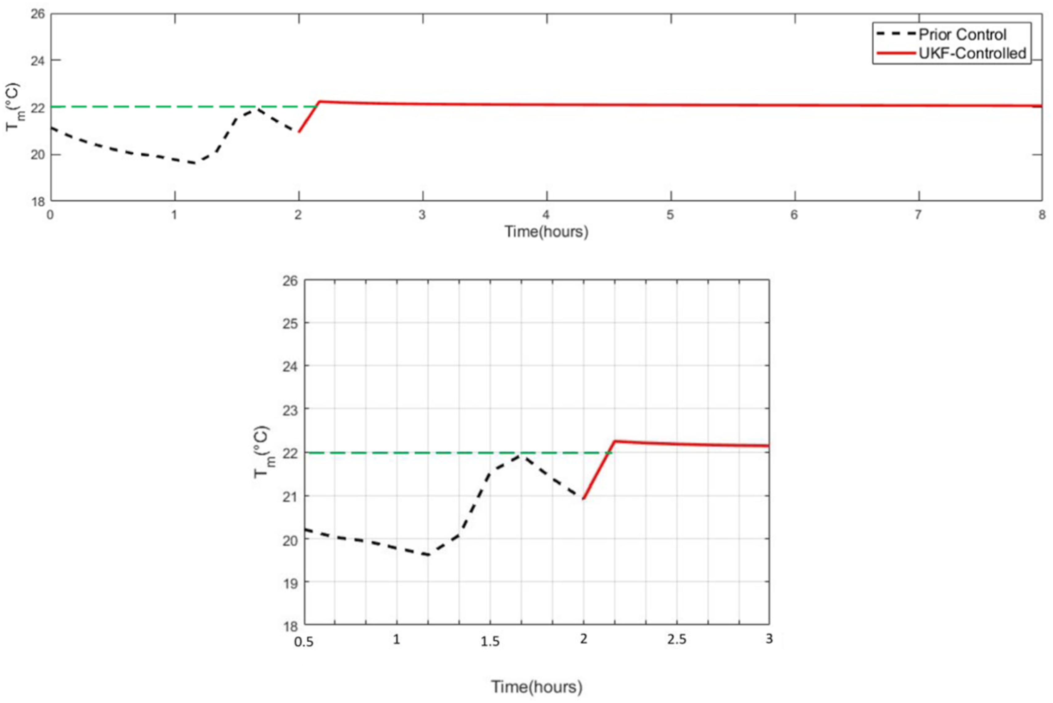
Scenario 10R6C-Ct2 focuses on controlling the temperature of multiple zones, specifically the main floor (Tm) and second floor (Tu), with estimation of corresponding heating and cooling supplies. To accomplish this, Qm and Qu have been added to the corresponding floor’s node (i.e., main and second floors). ODEs relating to this scenario are shown in Appendix B. The goal of this scenario is to maintain the temperature of the main floor at 23°C and the second floor at 22°C.
Figure 15(a) illustrates the estimated heating and cooling supply Qu which is used to control the temperature of second floor Tu at 22°C. Initially, the estimated Qu is 3.1 kW, but it varies between 0 and 0.5 kW to maintain Tu at the desired temperature. Figure 15(b) shows generated responses for Tu when estimated Qu is applied. It can be observed that Tu quickly increases from about 20.5 to the expected temperature (22°C) within the first 10 min and remains constant throughout the control dataset. (a) Estimated heating and cooling supply Qu, (b) Tu results in controlling dataset.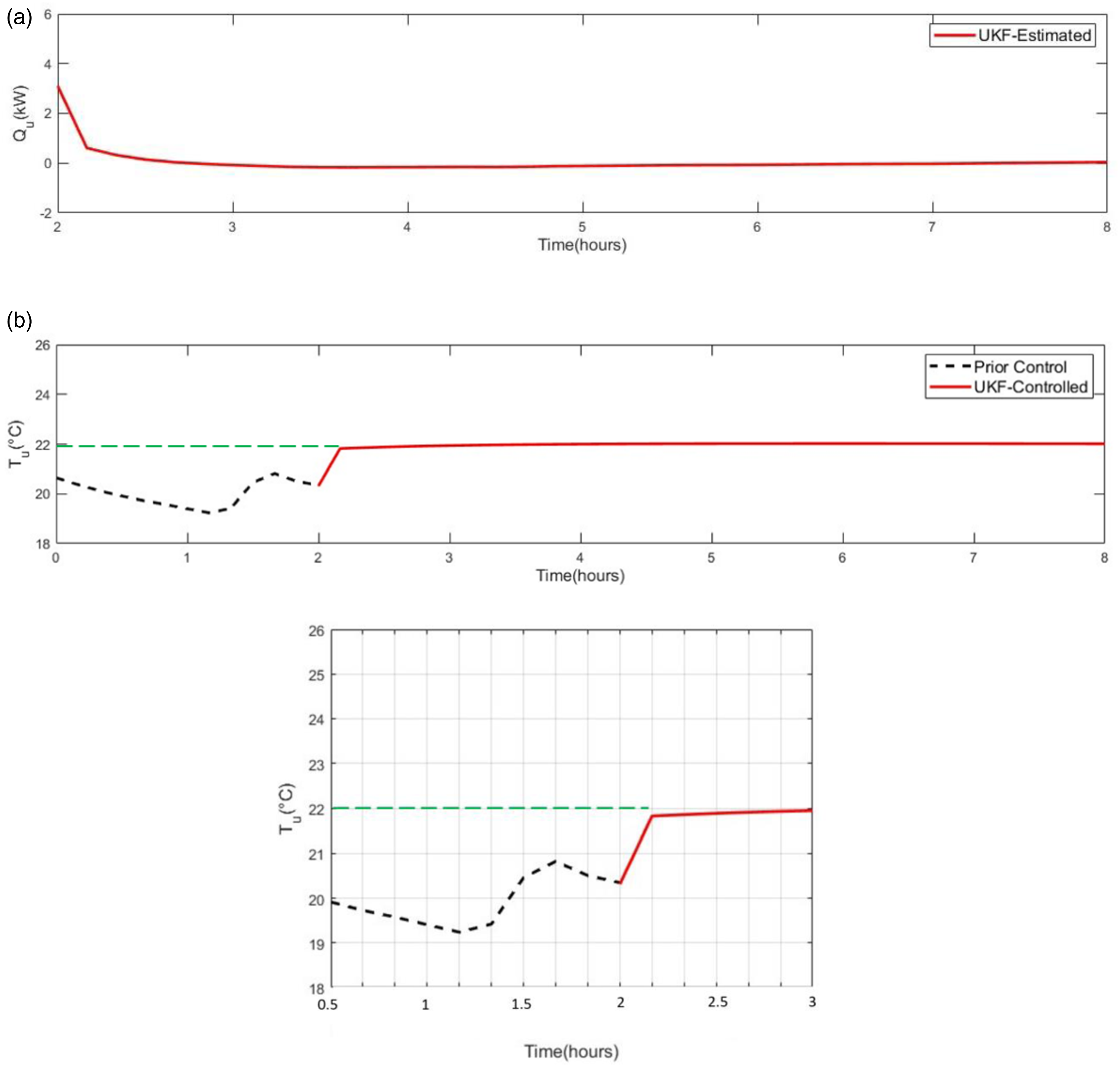
Figure 16(a) shows the estimated heating and cooling supply represented as Qm, used to control the temperature of the main floor (Tm) at a constant value of 23°C. The initial value of estimated Qm is 4 kW and it mostly varies between 0 and 3 kW to maintain Tm at the desired temperature. Figure 16(b) illustrates the generate temperature response of the main floor in the control dataset when estimated Qm is applied to the RC model. It is observed that Tm increases rapidly from about 21°C to 23°C in the first 10 min and stays at 23°C for the entire control period. (a) Estimated heating and cooling supply Qm, (b) results for Tm in a controlling dataset.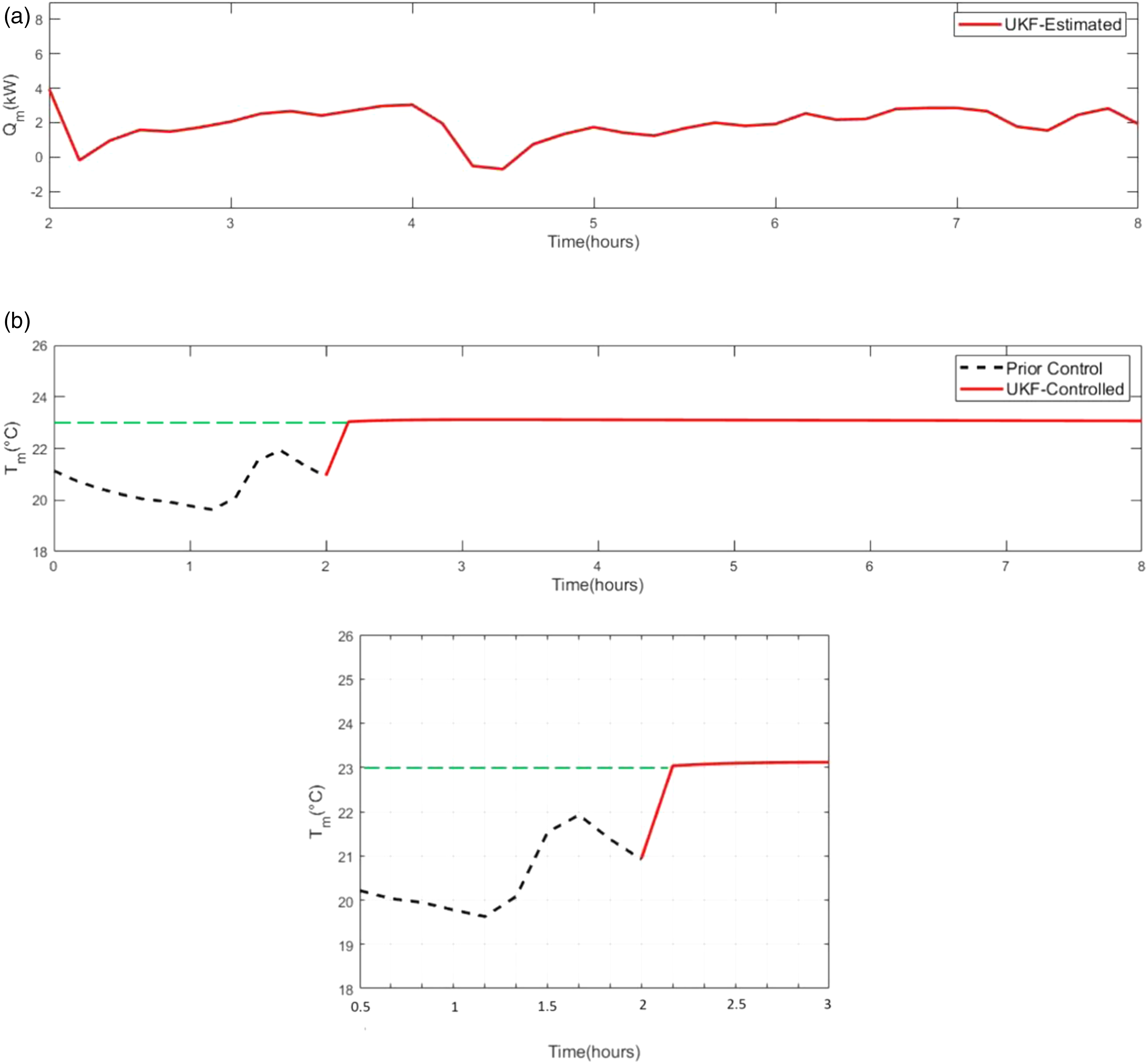
Conclusion
This study develops a method for estimating heating and cooling supplies (i.e., RC thermal model inputs) for temperature control purposes. In this regard, the method employs thermal resistor-capacitor network (RC) for thermal dynamic modeling and the Unscented Kalman filter (UKF), integrated with the Nonlinear Least Square (NLS) method, to estimate the heating and cooling supply. To evaluate the capability of the developed method, two application examples are presented: one using made-up data and the other using real-world data. Different scenarios, including limiting the maximum amount of the heating and cooling supply and controlling temperatures in multiple zones, are created to evaluate the capability and performance of the developed method in different circumstances. Implementing these equations manually may pose a challenge for architects or designers. Nevertheless, it is crucial to acknowledge that these equations form the basis for developing a specialized software tool in future works.
In the case study with made-up data, the estimated heating and cooling supply sharply drops the zone’s temperature from about 30°C to 26°C in the first 10 min and maintains that temperature for the remainder of the controlling dataset. Similarly, in the case of real-world data, the developed method accurately estimates the heating and cooling supply to control one and two zones. The considered zone temperatures reach the expected temperature set points of 22°C and 23°C in the first 10 min and remain constant throughout the controlling dataset. These accurate estimation of heating and cooling supply and controlling zone’s temperature on their expected level prove that the developed method is an effective technique for estimating heating and cooling supply of RC thermal models and can be used in control strategies.
Footnotes
Credit authorship contribution statement
Vahid Zamani: conceptualization, developing methodology, analysis implementation, and writing the original draft. Shaghayegh Abtahi: Manuscript revisions. Yong Li: supervision, conceptualization, and manuscript revisions. Yuxiang Chen: supervision, conceptualization, and manuscript revisions.
Declaration of conflicting interests
The author(s) declared no potential conflicts of interest with respect to the research, authorship, and/or publication of this article.
Funding
The author(s) disclosed receipt of the following financial support for the research, authorship, and/or publication of this article: The financial support for this research work is provided by Natural Sciences and Engineering Research Council of Canada (NSERC) Collaborative Research and Development Grants, CRDPJ 530932-18 entitled “Intelligent net-zero energy (ready) modular homes for cold regions.”