Sage Journals: Discover world-class research

Abstract

Unsteady behaviour of hydronic heating systems causes higher mean room temperatures than are required for comfort. Peak room temperatures depend on interactions between thermostats, heat emitters and the room. The importance of fluid properties on such unsteady heating is often misunderstood meaning potential energy savings are overlooked. This paper demonstrates the influence of fluid modifications and indicates a plausible magnitude of the energy saving opportunity. The results showed that fluid side heat transfer coefficient in isolation had negligible effect. Specific heat capacity of the fluid and flow rates were important, as they altered the amount of embedded energy in the heat emitter when thermostat conditions were met. Reductions in mean heating power for steady demand conditions were between 0 and 7% for plausible changes to fluid properties, depending on heat emitter size, room insulation and external temperature. Reductions in individual cycle energy were between 5 and 25%. When considered in the context of intermittent finite duration heating events, those that contained a small number of thermostat cycles demonstrated energy savings that tended towards the reductions in individual cycle energy. Heating events with larger numbers of cycles showed energy savings tending towards the reduction in mean heating power.

Keywords

Central heating zero-carbon buildings green buildings architectural engineering and sustainable development indoor thermal environment

Introduction

Society is facing a significant challenge in cost effectively meeting climate change emission commitments. The successful delivery of net-zero targets is widely accepted to need a portfolio of solutions whose cumulative contributions all play a part. UK building heat provision for industrial, commercial and domestic settings makes use of almost 560 GWh of energy,¹ approximately 30% of the UK’s energy demand. The decarbonization of space heating is therefore essential if net-zero targets are to be met. High costs and practical difficulties are limiting the rate of major overhauls of high CO₂ emitting heat provision in homes (e.g. gas boilers) with technologies such as heat pumps. However, much of the UK’s housing stock can be enhanced through energy efficiency measures which are lower cost and more accessible. To understand what opportunities for efficiency, exist, a clear and thorough understanding of the operation of heating systems is essential.

Heating systems are designed to provide comfortable conditions and achieving low energy consumption usually pushes objectives towards achieving the lowest comfortable environment temperatures. In many systems these ideal temperatures are only occasionally experienced.² Uncomfortably cold conditions would typically incur occupant intervention. Therefore, most of the operation of a satisfactory heating system typically occurs under conditions where the heat flow capacity (W) of the heating system exceeds that of the minimum required heating demand, often substantially. Most UK homes use central heating systems with hydronic heat distribution to heat emitters in individual rooms.³ Common technologies to match the heat provision to demand include timers, room/building thermostats and thermostatic radiator valves. Although more than 97% of dwellings in England had timers based on a 2011 study, only ∼50% of dwellings had the full set of heating controls.⁴ More advanced technologies such as smart controls are significantly rarer.

Even with timers, building thermostats and thermostatic radiator valves, under non-extreme conditions the rate of energy flow into the room through the hydronic system is significantly higher than the rate of heat loss to the surroundings which can be equivalent of 1^oC·hour⁻¹ with highly non-linear dependencies.⁵ It is not uncommon for heating and cooling flows, in the case of air conditioning systems, to be capable of rates of temperature change 5 to 10 times higher than surroundings heat loss/gains.^6,7 Even with a steady heat demand this creates a dynamic thermal environment where thermal energy is added to a space through the hydronic system until the flow is stopped when the room reaches its setpoint temperature (e.g. through a wall thermostat or thermostatic radiator valve, TRV). In the case of a moderate thermal inertia heat emitter, the heat emitter is now hot and continues to emit heat into the room causing the temperature to typically continue to rise before the heat loss dominates and the room starts to cool. Once the temperature is below the setpoint temperature the cycle can repeat. The importance of what may appear only small changes to such cycling behaviour can have a significant influence on energy consumption (circa 15%).⁷ In real-world scenarios where external temperatures, solar irradiance, meteorological conditions and occupant behaviours are fundamentally unsteady, the dynamic behaviour of the heating system is further exacerbated.

Smart thermostats with embedded computer control are being explored to better deliver against the heat demand. Model predictive controls and learning architectures have been shown to offer energy savings of 12–24% compared to more traditional controls without leading to reduction in comfort^8,9 or in some cases even increasing comfort.¹⁰ These energy savings are achieved through better optimized heat delivery. However, oscillations in room temperatures are still present^8,10,11 leaving opportunities for improved energy utilization.

The temperature of the space being heated is set by the occupant such that comfort conditions are met. This often sets a minimum temperature limit on the space and therefore, the lower temperature of the cyclic behaviour. Any temperature above this comfort level can be considered unnecessary and corresponds with excess energy provision and therefore, an opportunity for reduction in energy consumption. Fluid properties have a significant influence on the dynamic transfer of heat into the space and therefore changes to any such fluid properties can be considered to modify the unsteady transfer of heat. Such heat transfer modifiers can be expected to have an influence on the amount of excess heating and therefore, the amount of energy required to heat the space to threshold comfort levels. Despite the clarity in this logic argument, there are (to the authors’ knowledge) no explicit studies properly exploring the importance of fluid properties on room thermal management and energy consumption.

Within the technical community the authors commonly encounter claims that modifications to fluid properties cannot significantly reduce energy demand for space heating. This is leading to unnecessary barriers to the exploitation of the opportunities afforded by fluid engineering and thereby retarding our progress towards a net-zero society. For example, some assessment procedures explicitly exclude the dynamic effects on the system by recognizing only the impacts the fluid has on boiler efficiency.¹² For society to be able to leverage the potential CO₂ benefits of heat transfer modifiers, this position needs to be challenged.

This technical paper applies well accepted physical behaviours to a range of space heating scenarios to logically and clearly identify the flaws in such assertions. It provides an indication of the opportunity that exists for heat transfer modifiers to positively influence the heat demand whilst still delivering required space temperatures. It demonstrates fundamental differences between the effect of heat transfer modifiers and resizing the heating system.

Fluid properties that can influence unsteady heat transfer behaviour generally involve modifying one or more of the thermophysical properties of the fluid. The application of glycols to reduce the freezing point in heating systems is used to varying degrees around the world. The associated reductions in heat capacity and thermal conductivity, along with the increased viscosity are very much recognized to modify heat transfer.¹³ The impacts of drag reducing additives on heat transfer are more complex and although not widespread in space heating systems offer an avenue for heat transfer modification. Through the creation of larger structures such as micelles and micellar networks, turbulent mixing behaviours, as well as non-Newtonian viscosity behaviours not only influence the pipe pressure drops but also the heat transfer within the fluid.^14-16 On a molecular scale, surfactant surface affinity has been shown to influence near wall heat transfer.¹⁷ Although it is not the purpose of this paper to review every way in which heat transfer behaviour can be modified within a fluid, it is clear from the sample of literature referred to that modification of fluid heat transfer is not only possible but commonplace in a variety of existing applications. This paper, therefore, considers the impact of changes to heat transfer behaviours on the thermal-dynamic behaviour of an individual room.

Method

Although complex approaches such as neural networks are being explored for heating and cooling system thermal predictions with positive outcomes for objective oriented control,^10,18 the success of physics based numerical methods such as electrical-thermal analogies, makes them well suited to demonstrative studies such as this one. Non-linear auto-regressive models have been used for predicting building thermal behaviour which have suited the purpose of their study well,¹⁹ but without great effort only moderately capture the finer higher frequency response details of building behaviour. Such approaches require a significant body of appropriate experimental data which was both unnecessary and unavailable in the delivery of this study.

Lumped capacitance models are popular and prove excellent for exploring fundamental physical behaviours, provided care is taken in reducing the system into appropriate constituent parts. Such models have demonstrated good capability in predicting the cyclic unsteady behaviour of heating systems^9,20-24 provided energy flows are well accounted for.⁹ The rates of heating and cooling in particular have been clearly identified as being closely linked to the heat transfer to/from the walls,⁶ and therefore, the wall ‘skin’ thermal-dynamic behaviour. Through this link, the importance of building structure can be accounted for which has been shown to impact energy consumption results.²¹ The required fidelity of the wall is often incorporated into models through discretization of the wall layers such as that presented in Xu et al.²³ In some studies, the importance of the interior wall layers in comparison to the air thermal mass in the room is emphasized by the neglection of the internal thermal capacity of the room itself.²⁵ Some degree of simulation of the hydraulic heat emitter has also been shown to be important in predicting room thermal behaviour.²⁰ Lumped capacitance/electrical analogy modelling approaches have been used as a core part of stochastic modelling approaches to predict well the thermal behaviour of buildings.²² The success of lumped capacitance modelling with discretized elements makes it appropriate for use in exploring impacts of hydronic fluid properties.

The unsteady thermal model in this study incorporates a space (to be heated) and a hydronic heat emitter, represented diagrammatically in Figure 1. The space is considered to be well mixed and therefore a uniform temperature thermal mass which is thermally coupled to the radiator by a constant thermal resistance. For simplicity, the room floor plan is taken to be square, with a room height of 2.4 m. The interior wall surface is considered to represent current UK building approaches in which the inner skin of the wall consists of a plaster layer, taken as 15 mm thick for this model. The wall is discretized into 10 equally thick layers for which the energy flows are solved using explicit numerical approaches. The air side of the wall is thermally coupled to the room by a heat transfer coefficient of 8.5 W·m⁻²·K⁻¹ with plaster density, specific heat capacity and thermal conductivity of 800 kg·m⁻³, 950 J·kg⁻¹·K⁻¹ and 0.25 W·m⁻¹·K⁻¹ respectively. Any comparison made between cases with two different fluid properties has the same thermal resistance between the space and the radiator, and between the space and the surroundings. Equally, the surrounding temperature is kept the same between the cases and constant. This ensures that any effects evident in the comparisons arise from the changes on the water side within the heat emitter.

Figure 1.

Representation of the model domain.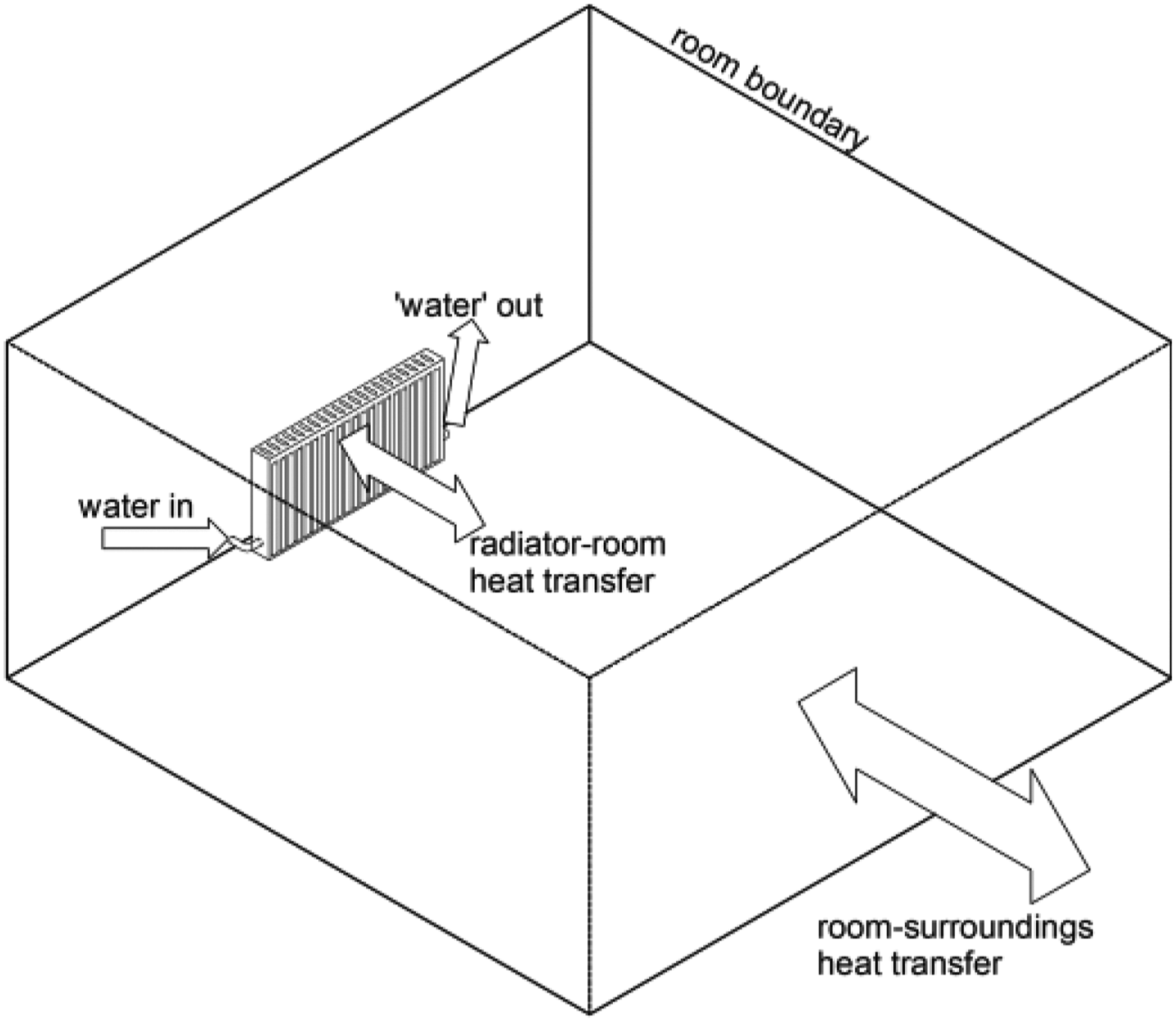

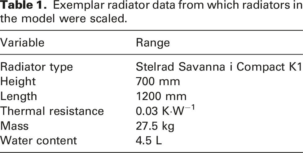
The radiator is divided into ten sections inside any one of which the fluid is considered to be well mixed, represented in Figure 2. The radiator wall is modelled independently to the liquid. The energy equation is solved explicitly for water and the radiator wall. Convection and convective heat transfer is accounted for on the water side with thermal resistances scaled from manufacturer data, shown here in Table 1.²⁶ The radiator sub-model considers solid conduction as well as convective heat transfer on the working fluid and air sides. This arrangement allows the model to incorporate a level of temperature heterogeneity within the heat emitter.

Figure 2.

Representation of the radiator model showing the discretization and heat transfer mechanisms considered.

Table 1.

Exemplar radiator data from which radiators in the model were scaled.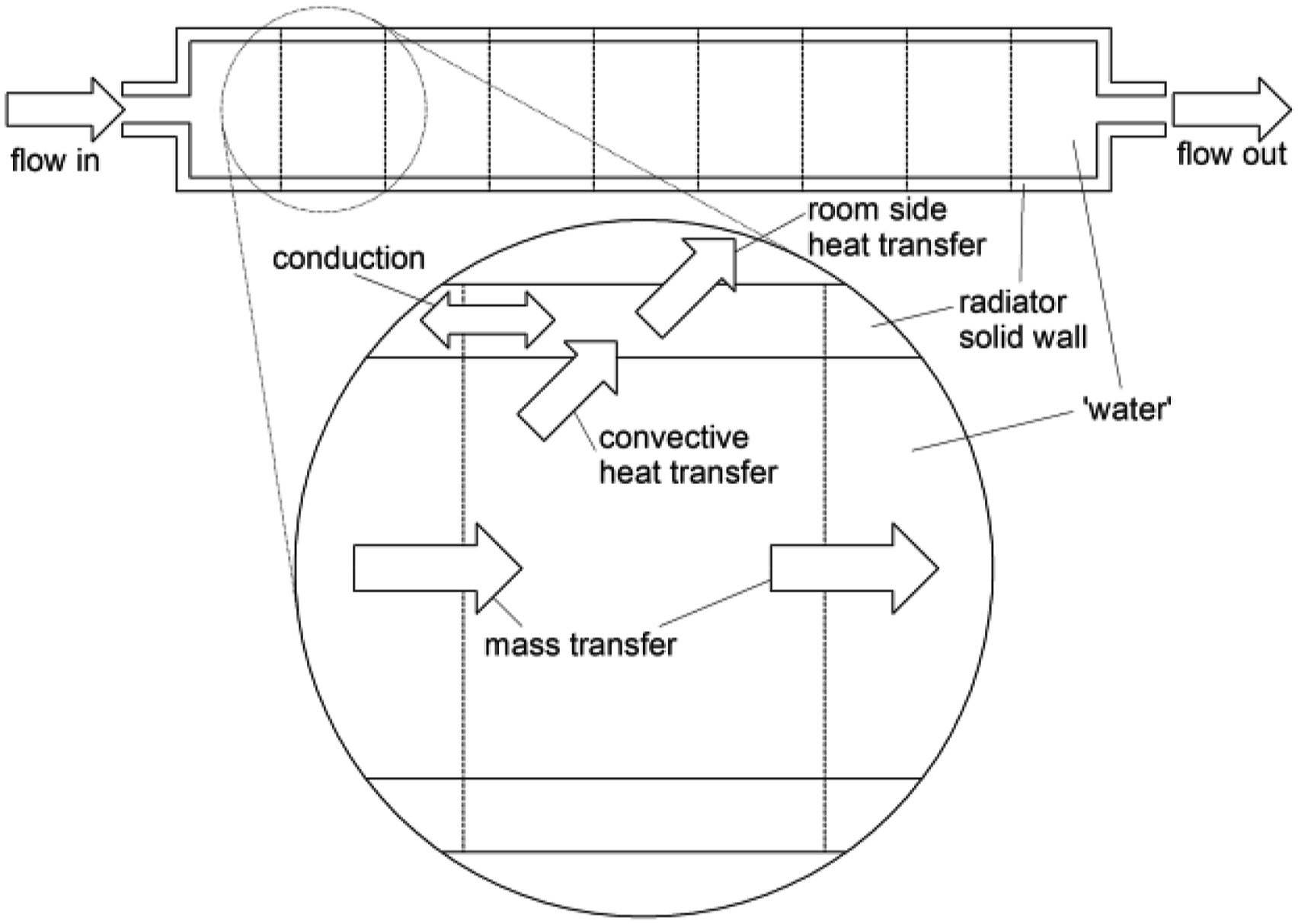

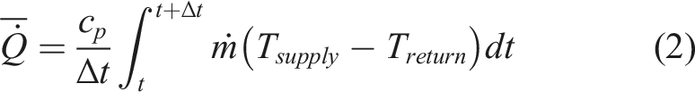
Variable	Range
Radiator type	Stelrad Savanna i Compact K1
Height	700 mm
Length	1200 mm
Thermal resistance	0.03 K·W⁻¹
Mass	27.5 kg
Water content	4.5 L

The net energy provided through the supply of water is calculated from the water flow using equation (1), where Q is the energy supplied, c_p is the specific heat capacity of the working fluid, $\dot{m}$ is the instantaneous mass flow, T_supply is the working fluid 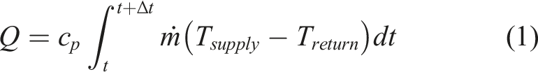temperature entering the radiator and T_return is the temperature of the water leaving the radiator. Where mean heating power is required, this is calculated as a time average using equation (2), where Δt is the duration under consideration.

Q = c_{p} \int_{t}^{t + ∆ t} \dot{m} (T_{s u p p l y} - T_{r e t u r n}) d t

(1)

\bar{\dot{Q}} = \frac{c_{p}}{∆ t} \int_{t}^{t + ∆ t} \dot{m} (T_{s u p p l y} - T_{r e t u r n}) d t

(2)

Where identified in the results, in situations where the boiler’s maximum heating power is less than that required to deliver the target supply temperature, the supply temperature will equal that provided by the maximum boiler capability. When the target supply temperature requires less energy than the minimum the boiler can provide, the fluid flow continues and the supply temperature is set to be equal to the return temperature.

The model incorporates a thermostatic radiator valve which linearly adjusts the mass flow rate between a maximum flow when the room temperature is at 19^oC, determined in practice, for example, by the pipe network design and pump, and zero flow at 20^oC representing a closed valve. This aligns with a valve authority of 1.²⁷ There is also a room thermostat that switches off the flow to the radiator once the room temperature has reached 20^oC.

Two scenarios are used within this report. The most common is that of a single pseudo-steady cycle in which the end thermal condition is equal to the start thermal condition. Such a modelled condition is representative of a repeating cycling process or pseudo-steady heating conditions. It is deemed representative of a continuous heating demand which is being controlled by a room thermostat. The second scenario is that of an initial cycle where the space, radiator and working fluid begin at a fixed initial temperature and are heated until the thermostat demand has been met and the room temperature has dropped to 19^oC, a condition which would then demand more heat. This condition is taken as representative of an initial heating cycle. When a finite heating duration is discussed, it refers to an integer number of heating events where the first is from the start condition and subsequent heating events are from the pseudo-steady cycle scenario.

Water supply temperature, radiator length, room thermal mass, surroundings temperature, room-surroundings steady state thermal resistance (i.e. degree of insulation) and maximum radiator flow rate are all considered as variables that have been explored to give an indication of a range of reasonable conditions arising from differences in housing stock and meteorological conditions. When looking at the opportunity for energy saving, these variables have been randomly selected for each case within a predefined range so that results are not solely applicable to a singular scenario.

Experimental validation

Validation data was captured as part of a separate project from the unoccupied 2010 BRE Exemplar House at Liverpool John Moores University (UK). The house is typical of a UK 3-bedroom end terrace property built in 2010. It has a combination condensing boiler providing hot water and heating on demand to the property. The heating system includes 3 min of no-added-heat circulation once the thermostat demand ends.

A radiator was fitted with a UF08B100 Cynergy ultrasonic flow meter. A 1.5 mm K-type thermocouple was inserted in the radiator inlet and outlet flows, thereby allowing calculation of heat provision to the radiator through the water flow. The room temperature was measured near the centre of the floor plan at a height of 1.6 m from the ground. The radiator characteristics were assumed to match those of the radiator in Table 1, and the room size and internal mass was calculated from the room geometry and estimated for the furniture.

Initial conditions were taken from the experimental data, along with the peak water supply temperature. The water supply temperature in the model was assumed to be constantly at the peak value and does not, therefore, consider the gradual heating of the provision water.

Figure 3 shows a comparison of the models predicted flow temperatures at the inlet end and outlet end of the radiator. As the water temperature entering the radiator changes instantaneously in the model, it is appropriate in this comparison to include an offset where the hot water provision in the model begins at ∼50% of the rise in inlet temperature of the water in the experimental case. During the heating phase, the radiator temperature predictions match well with the experimental data. When the no-heat circulation begins, the predicted inlet radiator temperatures show a rapid drop as the outlet temperatures continue to rise, as seen in the experimental data. Both the simulation and experimental data show a small ‘bump’ in the temperatures peaking at the point the flow stops. The peak of the bump and subsequent decline of the temperatures was more rapid in the experiment, however, this is not unexpected as the experimental temperature was measured in the pipe adjacent to the radiator and therefore had a significantly smaller heat capacity than the model location which was just inside the radiator. For the purposes of this study, which requires the model to reasonably represent significant real-world processes, the model of the radiator is appropriate.

Figure 3.

Comparison of flow rates and water temperatures between the experimental data and an equivalent model scenario. Solid lines represent the model data. Broken lines represent the experimental data.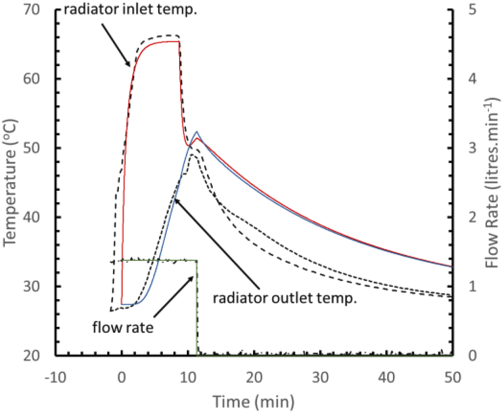

Figure 4 shows the predicted room temperature during this heating event. There is an offset in the data which is expected to arise from heterogeneity in the room temperature during heating which is not represented in the model. This may lead to time lags and minor variations in the room temperature measurement which would not exist in the ‘well-mixed’ model case. Importantly the rate of temperature rise of the room and rate of temperature decay are predicted well which indicate that the thermal coupling between the radiator and the room, and the room and the wall/surroundings is reasonable.

Figure 4.

Comparison of the experimental and modelled room temperatures for the validation case. Solid line represents the model data. Broken line represents the experimental data.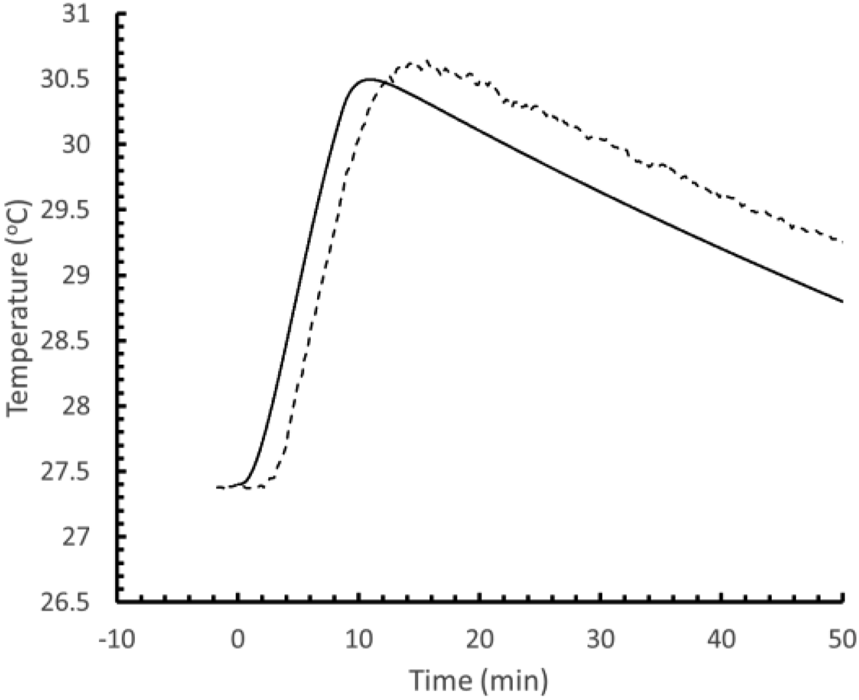

Figure 5 compares the input energy prediction calculated based on the specific heat capacity, flow rate and temperature difference across the water supply and return to the radiator. The prediction of the energy consumed is good, indicating that the heat transfer between the water and the radiator, and between the radiator and the room are reasonable.

Figure 5.

Comparison of the experimental and modelled cumulative energy transfer via the water flow to the radiator.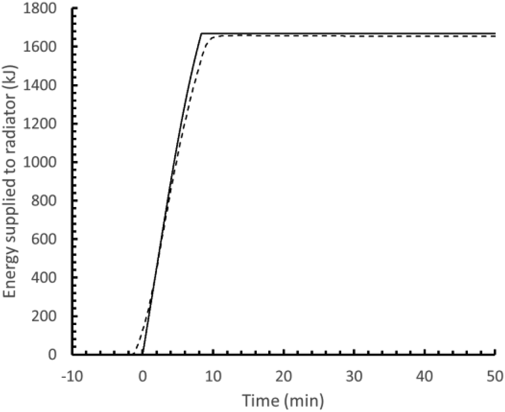

This validation gives confidence that the fundamental behaviours of the radiator and room are captured in this model. Although the complexities of room heat distribution have not been explored here, that part of the model is kept consistent between comparisons with only the fluid side of the radiator being subjected to change. Therefore, this model is deemed suitable for exploration of ways in which fluid side properties can influence the provision of heat.

Results: Influence of fluid properties

The following results consider the pseudo-steady scenario which indicates the impacts of changes on mean heating power for a steady heating demand. As this is a cyclic process, there must be a net balance of the energy added through the working fluid and the energy lost through the space-surroundings thermal coupling. As the space-surroundings thermal resistance is fixed in any comparison, the impact of changing the fluid properties on the heating power required can only manifest through changing the room or wall skin layer temperature.

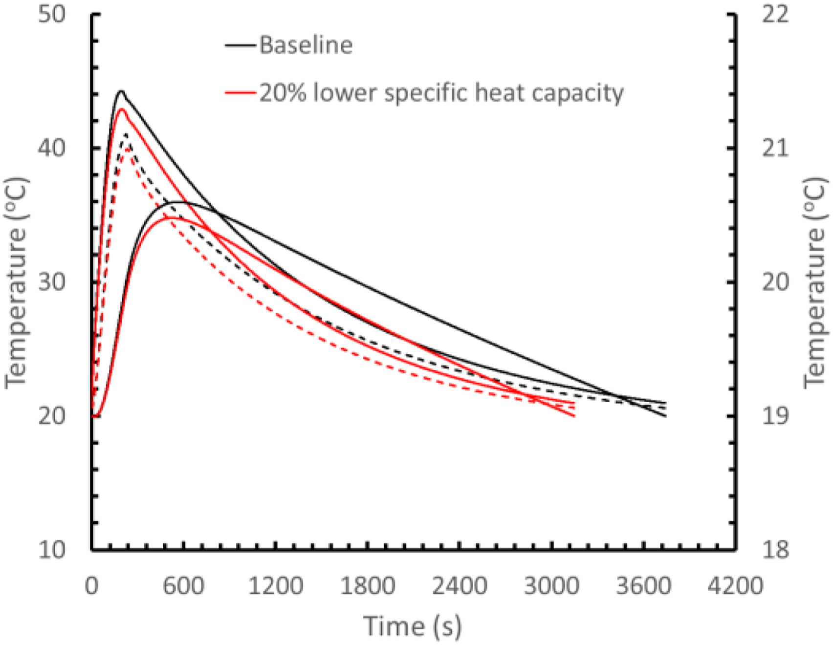
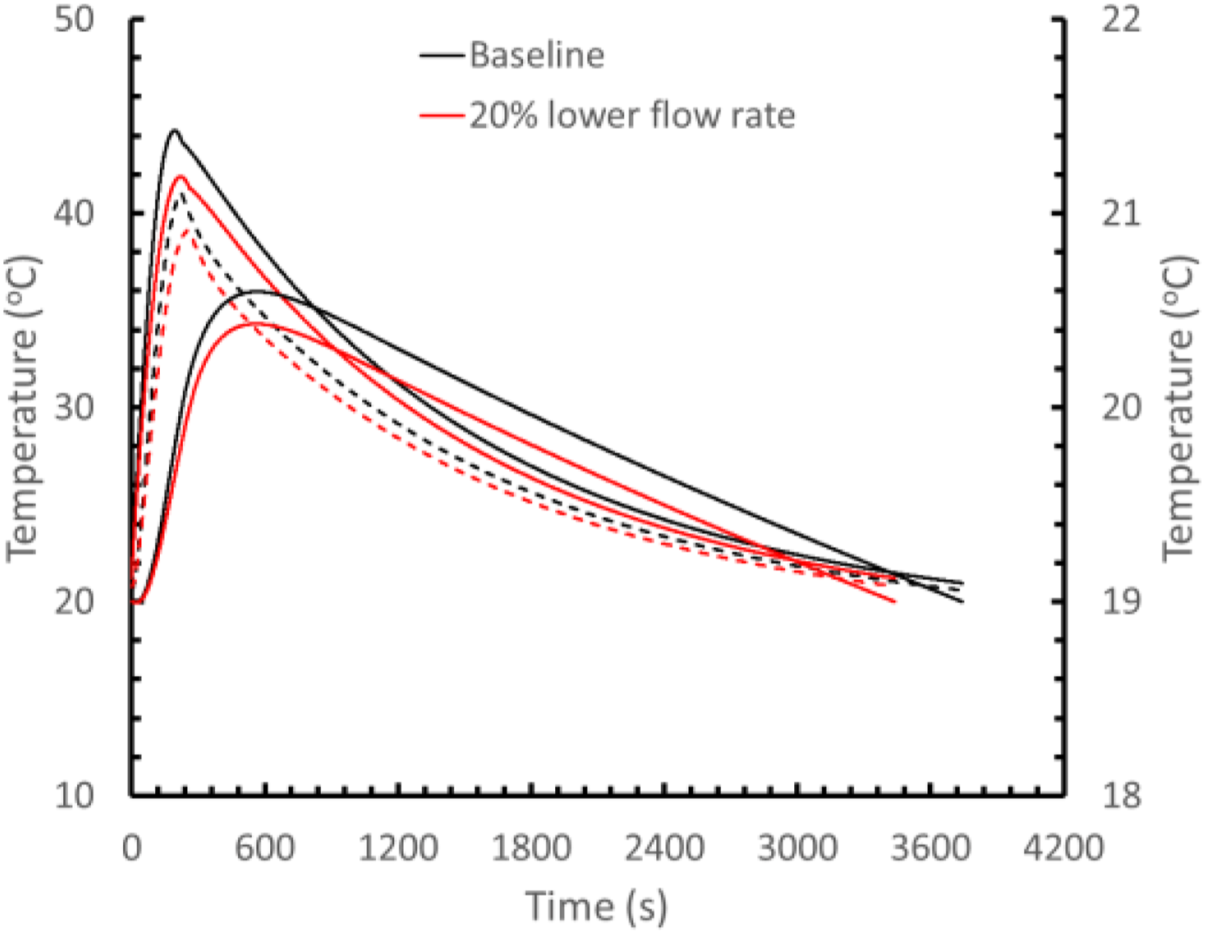
The impacts of heat transfer coefficient, heat capacity and viscosity were explored independently for different flow rates, external temperatures and supply water temperatures. It is acknowledged that these variables are not always independent. However, it is useful to consider the effect of heat transfer coefficient separately to help isolate the relationships. Heat transfer coefficient, for example, could be varied independently by introducing turbulence sources. The first results presented (Figures 6–8) have no limits imposed on the amount of heating power that the boiler can provide to deliver the required supply fluid temperature.

Figure 6.

Impact of 50% higher fluid side heat transfer coefficient on mean fluid , radiator wall and room temperatures.

Figure 7.

Impact of 20% lower fluid heat capacity on mean fluid (left axis), radiator wall (left axis) and room temperatures (right axis).

Figure 8.

Impact of 20% lower fluid flow rate on mean fluid (left axis), radiator wall (left axis) and room temperatures (right axis).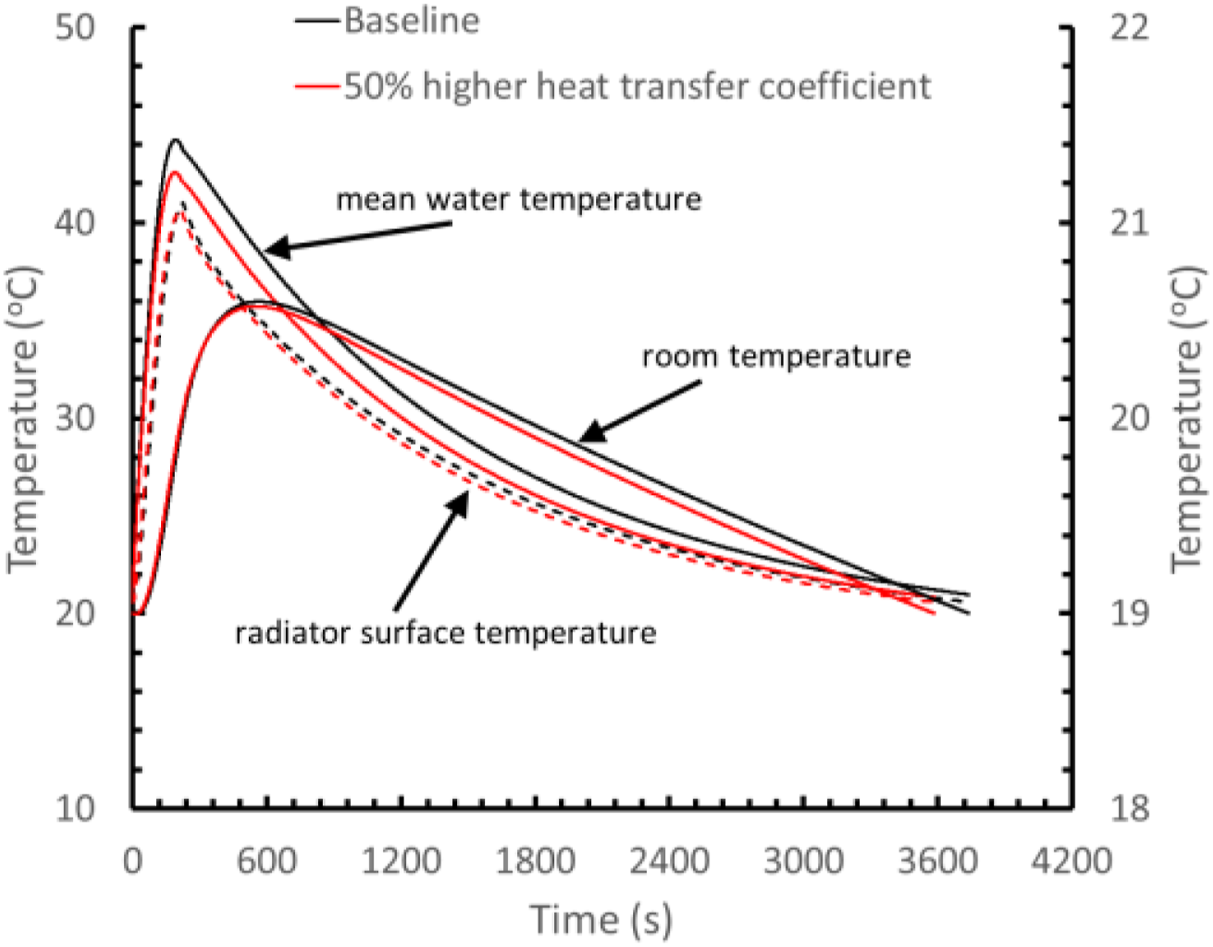

An example of the influence of a 50% increase in the fluid side heat transfer coefficient on mean fluid temperature and radiator wall temperature is shown in Figure 6. A small change in mean water temperature is visible, which belies the larger changes in temperature distribution across the radiator surface. The higher heat transfer coefficient causes the heat to move more quickly from the water into the radiator surface. However, the amount of energy available to the radiator in the early heating stages is the same, resulting in very little change in the mean radiator surface temperature and therefore the heat transferred to the room is very similar between cases. The result is only a marginal change in room temperature through the cycle and the mean heating power changing by <1% around zero, depending on simulation input parameters.

It is reasonable therefore to conclude that in such hydronic systems, changing the heat transfer coefficient on the fluid side in the absence of any other properties changing has a relatively small (and typically insignificant) effect on the heat flow into the space and therefore the energy demand. Importantly, however, heat transfer modifiers do not change heat transfer properties in isolation, but include effects of changes to kinematic viscosity, specific heat capacity and thermal conductivity. Although the thermal conductivity might initially be conflated with the heat transfer coefficient alone, the heat capacity and viscosity changes can significantly influence the rate of heat delivery in their own right, and therefore can have additional impacts.

Figure 7 shows an exemplar impact of a 20% reduction of fluid heat capacity on fluid, radiator wall and room temperatures. The lower heat capacity means that the supply water cools more quickly as it enters the radiator, resulting in the rate of rising of radiator temperature and peak radiator temperatures marginally reducing. The rate of increase in room temperature is also slightly reduced, however, the most significant factor is in the amount of embedded thermal energy within the radiator, specifically the encompassed fluid, at the time the thermostat switches off the heating demand, that is, when the room temperature reaches 20°C. This causes the peak room temperatures to be noticeably lower. The cycle duration is equally reduced, but the drop in the mean room temperature is equivalent to a 10–30% reduction in mean heating power required, dependent on the input conditions used. This impact is significant and with such changes in heat capacity being plausible, must be considered further.

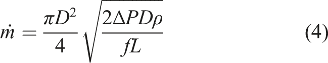
The fluid flow in a heating pipe network encompasses a large range of Reynolds numbers from low to moderate. The lower flows are encountered rather frequently due to the throttling effect of thermostatic radiator valves, as they approach their closing temperature. The dynamic viscosity and density will be the main contributors to changing flow rate in the pipe network which will influence the maximum flow through the network. Where velocity is related to pressure and fluid properties by a friction factor, f, as shown in equation (3) where ΔP is the total pressure drop, L is the pipe length, D is the hydraulic diameter, ρ is the fluid density and V is the fluid velocity, then the mass flow would be related to conditions as shown in equation (4). 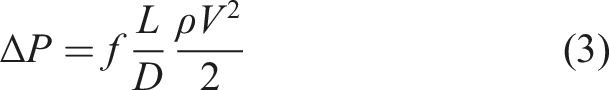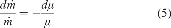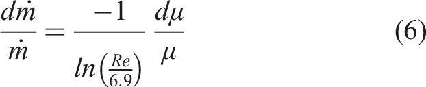Under laminar flow conditions when the friction factor is close to 64/Re, where Re is the Reynolds number of the flow, the relationship between changes in dynamic viscosity μ and mass flow rate $\dot{m}$ can therefore be shown to be as in equation (5) which indicates that a percentage change in viscosity will correspond to an equal percentage change in mass flow. For turbulent flows where Re is relatively low and the Haaland approximation for friction factor is used, it can be shown that equation (6) holds true making the magnitude of the coefficient linking mass flow changes to viscosity changes to be between 0.13 and 0.16 for typical heating system Reynolds numbers.

∆ P = f \frac{L}{D} \frac{ρ V^{2}}{2}

(3)

\dot{m} = \frac{π D^{2}}{4} \sqrt{\frac{2 ∆ P D ρ}{f L}}

(4)

\frac{d \dot{m}}{\dot{m}} = - \frac{d μ}{μ}

(5)

\frac{d \dot{m}}{\dot{m}} = \frac{- 1}{\ln (\frac{R e}{6.9})} \frac{d μ}{μ}

(6)

Depending on the heating system design, we can expect a percentage point change in dynamic viscosity to have between a 0.13% and 1% point change in mass flow depending on the flow conditions. Without worrying about the more subtle contributions to pressure losses, it is clear that significant viscosity changes possible from changing fluid properties can have a significant influence on the flow rate in heating systems.

The impact of a 20% change in flow rate on the energy required was between 4 and 13% depending on simulation conditions. An example is shown in Figure 8. The effect of a change in mass flow is to change the rate of energy input to the heat emitter during the heating phase, in addition to reducing the embedded thermal energy within the radiator once the setpoint temperature has been reached and the fluid circulation stops. The result of this is a lower average room temperature and therefore a reduction in the mean heating power required.

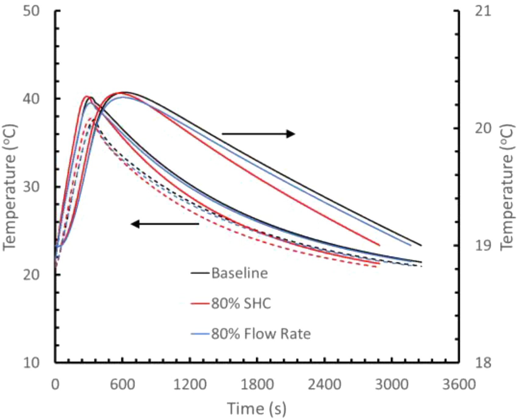
The results presented thus far have not considered any limitations on the amount of heating power that can be put into the working fluid. Practical boiler designs have upper and lower limits on the rate of heat they can add which are dependent on the burner and boiler design. How this impacts individual radiator supply depends on the distribution of the working fluid between radiators. Two cases are considered here to understand if the heat input rate limits significantly interact with the effect of heat capacity and flow rate. The first is one representative of a relatively small boiler supplying all the radiators at the same time, therefore, the maximum rate of heat provision to an individual radiator will be a fraction of the maximum boiler power. In the example in Figure 9, this is taken as 3000 W for the radiator in question. The minimum sustainable heating power is 300 W based on a 10% minimum modulation of the boiler’s burner. The second case, also shown in Figure 9, considers a situation where most of the system flow is going through only the radiator in question resulting in the maximum heating power being closer to the boiler power rating. This is taken as 20 kW for the purposes of this example. The minimum in this case was set at 2 kW based on a 10% modulating burner limit.

Figure 9.

Impact of boiler heating power limits on mean fluid, radiator wall and room temperatures.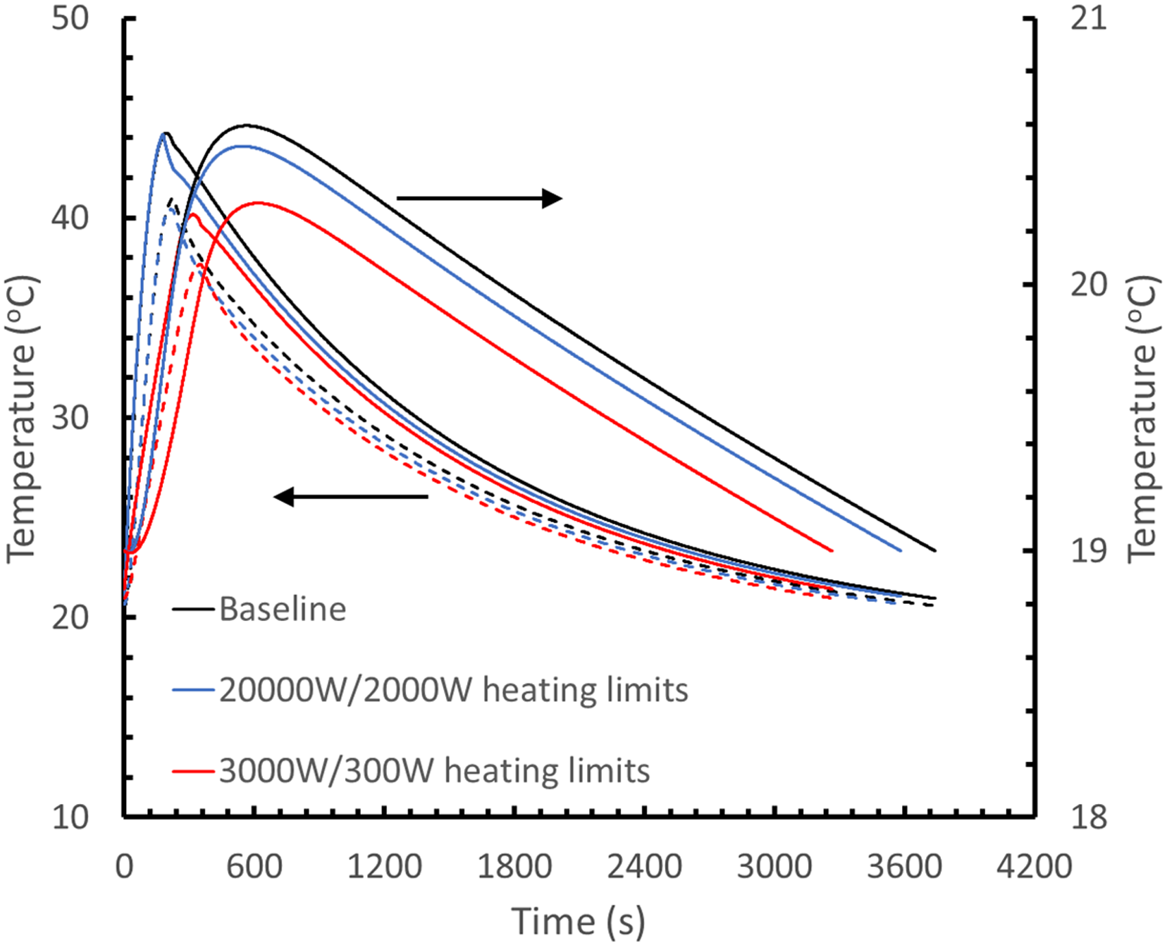

It is apparent in Figure 9 that the former case with a 3000 W upper heating power limit varies from the baseline case in its initial rate of heating. The water provided is at a lower temperature for a longer period, which reduces the initial rate of warm up and consequently the peak temperatures of the room. The latter case is affected by the lower heating power limit which causes the heat addition to cut out before the temperature demand has been met, whilst the fluid continues to circulate. This results in an initial stage of the cycle which is the same as the baseline but, due to less embedded energy in the radiator when the thermostat trips off, the peak room temperatures are reduced.

Figures 10 and 11 show the effects of changes in heat capacity and mass flow on the dynamic thermal behaviour of the room. The results remain consistent with previous observations, however, because the rate of heat input to the radiator is limited by the 3 kW limit in the case of Figure 11, the impact of the fluid is smaller. The impact on mean room temperature is more significant in the cases with the 20 kW and 2 kW upper and lower limits. Although it is not clearly visible in Figure 11, the rate of rise of mean and peak temperatures of the radiator are ∼17% and >35% higher than the baseline, which translates in this particular case to a faster heating of the room, to the point the thermostat stops demanding heat. This may offer some additional perceived benefits.

Figure 10.

Effects of reduction in specific heat capacity (SHC) and mass flow on temperature for upper and lower heating power limits of 20 kW and 2 kW, respectively.

Figure 11.

Effects of reduction in specific heat capacity (SHC) and mass flow on temperature for upper and lower heating power limits of 3000 W and 300 W, respectively.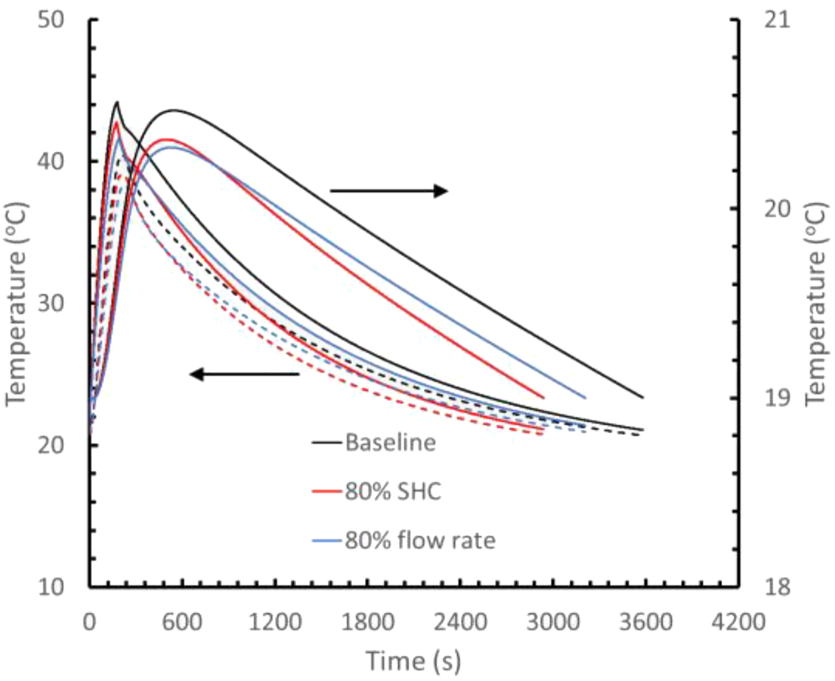

Variables in the simulation relating to the building, radiator or surroundings have been varied independently from the central conditions previously presented to ascertain directional trends. The results are shown in Figure 12. This suggests that there is more fractional opportunity under mild conditions in systems with high water supply temperatures and relatively high flow rates. Absolute energy savings are better considered later in this study, but this does demonstrate clear interactions between the system, building and fluid.

Figure 12.

Influence of changing input variables on the mean heating power demand for the room.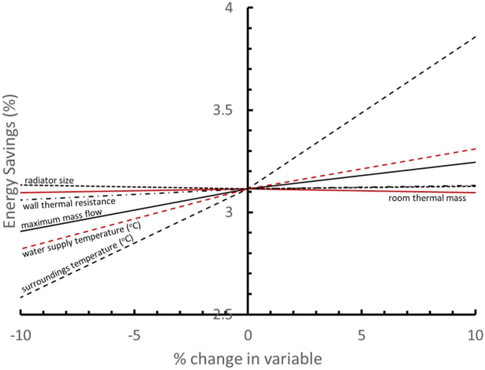

The clear importance of building fabric, system designs and external conditions on determining the scale of opportunity for energy saving, therefore, requires a Monte-Carlo type approach to quantifying the opportunity.

Results: Energy saving opportunity

Four different fluid characteristics were considered. The first was the baseline which had properties representative of water. There were then three modifications of this identified by their change to heat transfer coefficient, specific heat capacity and flow rate. For example, the samples denoted 95/90/90 have 95% of the heat transfer coefficient of the baseline case, 90% of the specific heat capacity and a viscosity that results in 90% of the flow rate for any given condition. It is not intended that these are specific fluids, but only as feasible examples to demonstrate the potential impact that changing unsteady heat transfer related properties can have.

The non-fluid inputs for the simulations were then randomly varied across predefined ranges with 200 cases for each fluid comparison. The actual range of input data used across the simulations presented is shown in Table 2. The mean heating power input and the individual cycle energy were then compared to that of the baseline fluid and the changes plotted in Figure 13 and 14, respectively. They have been plotted against the ratio of the rate of heat loss from the room at the demanded temperature to the maximum heating power of the heat emitter, which somewhat characterizes the amount of oversizing of the heat emitter for that given condition. This is calculated as shown in equation (7).

H e a t f l o w r a t i o = \frac{R_{e - r} (T_{d e m a n d} - T_{\infty})}{R_{r - \infty} (T_{s u p p l y} - T_{d e m a n d})}

(7)

where R_e-r is the indicative thermal resistance between the fluid in the heat emitter and the room, R_r-∞ is the thermal resistance between the room interior and surroundings, T_demand is the indicative setpoint room temperature, T_supply is the maximum supply temperature and T_∞ is the surroundings temperature.

Table 2.

Input data summary.

Variable	Range	Mean
Water supply temp	60.0–80.0^oC	70.4^oC
Radiator length	0.50–1.50 m	1.01 m
Room thermal mass	25–301 kJ·^oC⁻¹	91.6 kJ·^oC⁻¹
Surroundings temperature	1.0–17.0^oC	8.3^oC
Room-surroundings thermal resistance	0.020–0.050 K·W⁻¹	0.035 K·W⁻¹
Maximum rad. flow	72–180 L·h⁻¹	123 L·h⁻¹

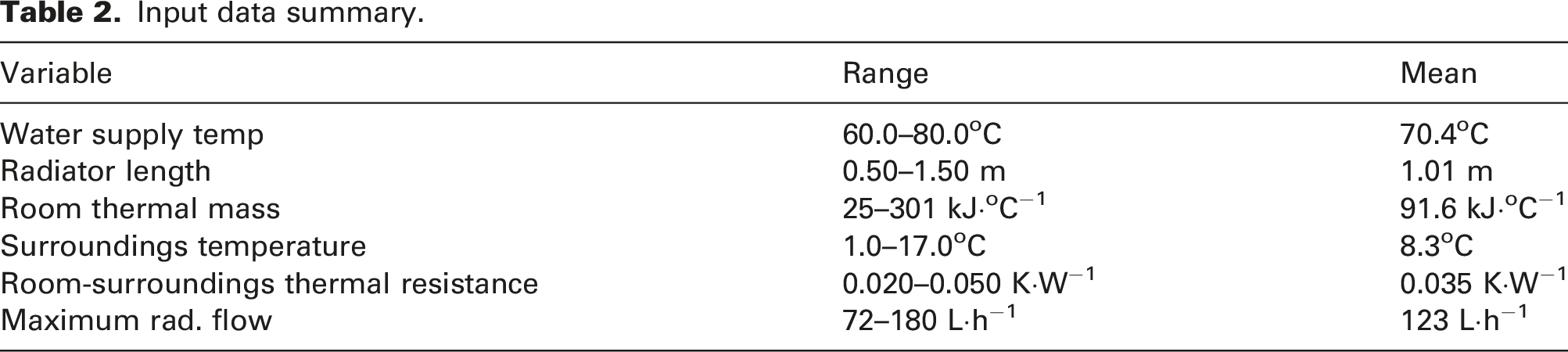
It is immediately apparent looking at Figure 13 that there are few conditions for which energy delivered to the room to achieve the temperature demand is increased by the changes to the fluid side conditions, induced by the reductions to fluid specific heat capacity and mass flows in particular. The cases that show marginal increases are over by a magnitude comparable to the numerical errors in the calculation. The amount of reduction in heating demand for the room increases as the ratio of heat demand to maximum heat supply reduces. This can happen as a result of better room insulation, larger heat emitters or milder external temperatures. The secondary effects result in a spread of data points, but the trend remains visible. The more significant the reductions in flow and fluid specific heat capacity are, the bigger the impact on the excess heating of the room. Such changes in fluid properties which are feasible with existing heating system fluid additives can be seen to offer 0.5–7% reduction in mean heat power demand across the range of input data used, but importantly showing consistently a benefit.

Figure 13.

Mean heating power changes resulting from three different conceptual fluids resulting from the Monte-Carlo simulation.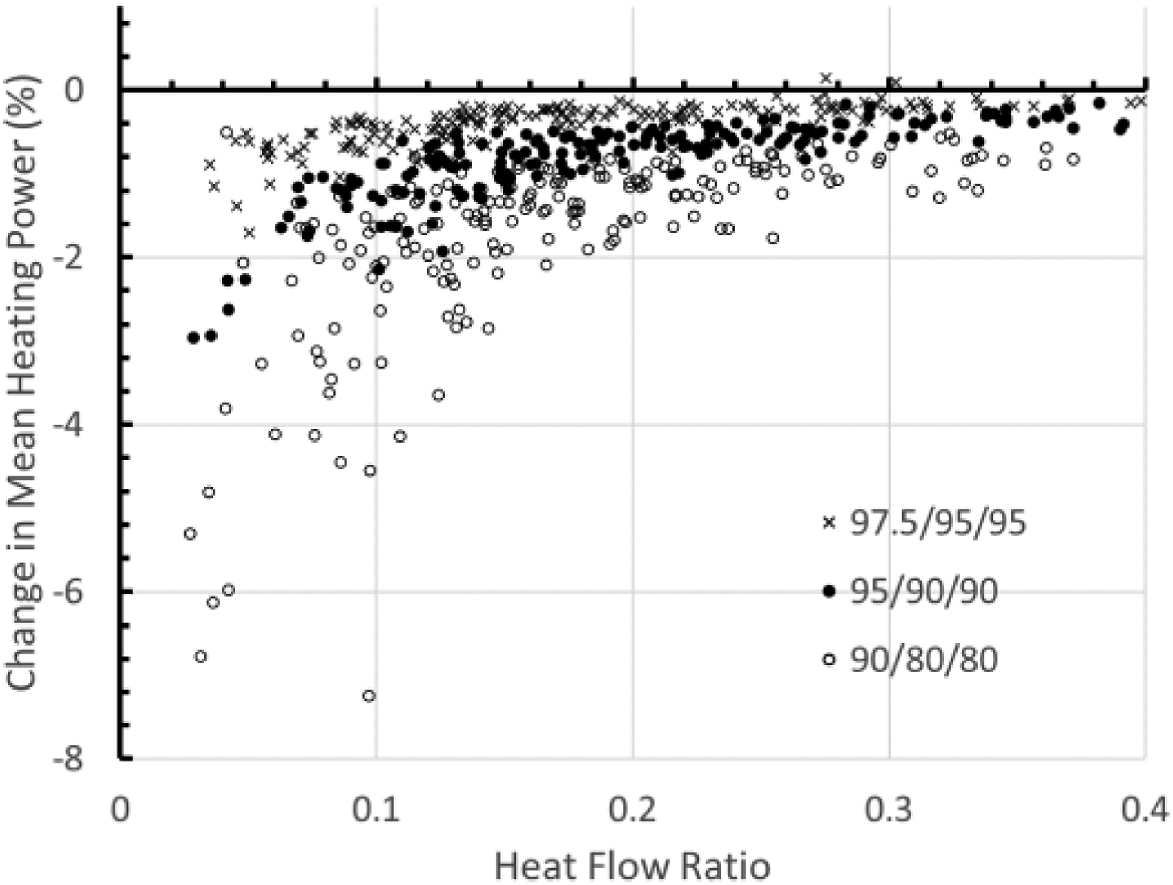

An exemplar end of terrace new build property may have a thermal resistance ∼0.01 K·W⁻¹. Accounting for the internal generation and therefore heat demand identified using SAP protocols, the ratio of demand to maximum heat flows is, based on monthly averages, between 0 and 0.064, with 90% of the heating energy consumed at ratios between 0.02 and 0.064 (note the exact ratios depend on radiator sizing). Although these are monthly means, typical extremes in temperature will expand this ratio upwards no more than 50%. The left-hand side of the plots can therefore be expected to be more representative of current standard buildings.

The impact of the demand to maximum heating ratio on the change in individual cycle energy is less significant, as seen in Figure 14. However, the changes in the energy per cycle are larger by a factor of ∼4 than the changes in mean power previously shown. The more extreme the change in fluid properties the larger the potential change to cycle energy.

Figure 14.

Cycle energy demand changes resulting from three different conceptual fluids resulting from the Monte-Carlo simulation.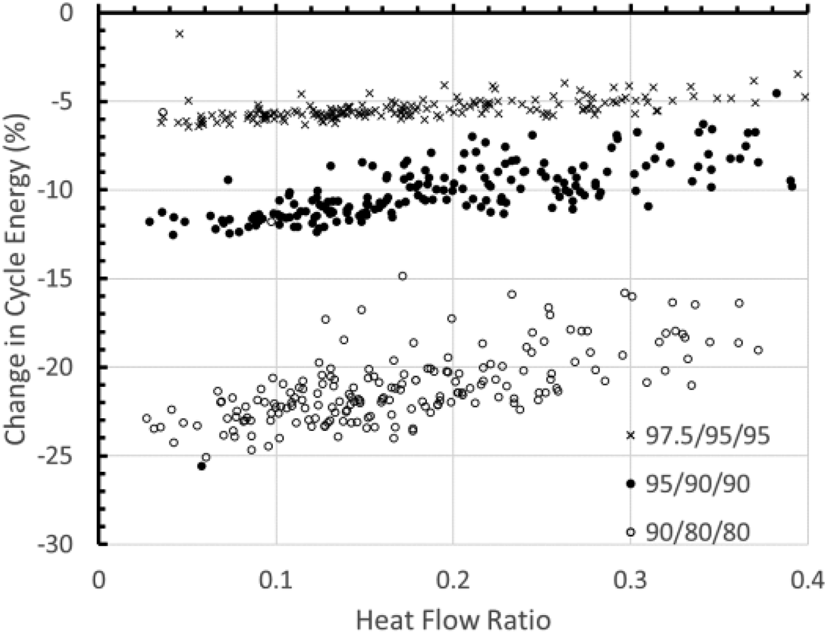

When considering the opportunity across a portfolio of buildings under a variety of external conditions, the effect of finite heating events also needs to be considered. For example, if heat was demanded for a period of only 1 h then a single heating event would occur in most cases. The mean heating power in such a scenario becomes irrelevant with regards to the amount of energy used, instead being determined by the single cycle energy consumption, characterized by the results in Figure 14. As the heating event increases in duration and there becomes a very large number of ‘steady’ demand cycles, the change in energy consumption would tend towards the values characterized by Figure 13.

One-hundred randomized sets of input data were used for each of the conceptual modified fluids to predict the energy saving potential of such 100 heating events as a function of their duration. The range was almost identical to those presented in Table 2. The change in energy used is the change in total energy consumed by the 100 heating events, not a mean of the percentage benefits, therefore, it has not been unduly biased towards milder conditions where less energy is used. The first of any series of heating cycles was calculated based on a uniform initial temperature representing an initial warmup of the space. Data showing individual scenarios making up the net energy change are presented in Appendix A for a selection of heating durations and each of the fluids, showing the characteristics spread of the data one might expect if experimentally studying such effects. The shorter durations offer benefits tending towards the change in individual cycle energy consumption. As the duration increases, the number of heating events using the modified fluids which have an additional heating cycle when compared to the baseline slowly increases. When an additional cycle is present for the modified fluid case in comparison to the baseline, the amount of energy consumed is significantly higher. It is such events that are responsible for bringing the average benefit back down towards the ‘steady’ heating mean power. Such characteristic behaviour makes clear why when testing over a duration which experiences different external conditions, a large spread in the energy consumed in individual heating events (or e.g. days) should be expected. This is often misconstrued as demonstrating inconsistent effects which cannot be attributed to the fluid, yet here such effects are clearly apparent in a calculation where the only change is the fluid. Figure 15 shows the energy consumption change across the cases, which had demand to maximum heating ratios between 0 and 0.2 presented for each fluid as a function of heating duration. It becomes more apparent here, particularly with the larger fluid property changes, that the short duration event benefit tends towards the cycle energy reduction (Figure 14), whilst the longer heating event benefit tends more towards that of the ‘steady’ heating cycle (Figure 13).

Figure 15.

Net change in energy used across the portfolio of 100 scenarios for the three fluids as a function of the duration of the heating demand.

Results: Impact on Heating Capacity

It is useful to consider such fluid property changes in the context of the heating capacity of the heat emitter, that is, how much heat flow it can deliver under extreme cold conditions. The ratio of extreme heat output reduction to fuel savings at a heat ratio of 0.05–0.15 is ∼1.2. This means that for the fluid properties shown here, a 1% reduction in energy use under normal conditions coincides typically with a 1.2% reduction of maximum heat output of the heat emitter. This may suggest that the effects demonstrated in this paper are akin to installing a smaller radiator. For these scenarios, the simulation tool was used to determine what reduction in radiator size would offer the same benefit under normal conditions. The comparison of using the fluid to achieve this saving versus using the radiator to achieve the saving is summarized in Figure 16. It is immediately apparent that the fluid property modifications have a substantially smaller effect on the extreme condition performance of the radiator, by a factor of typically 4–8.

Figure 16.

Comparison of the loss of heating capacity arising from radiator size reduction to that of modifying fluid properties.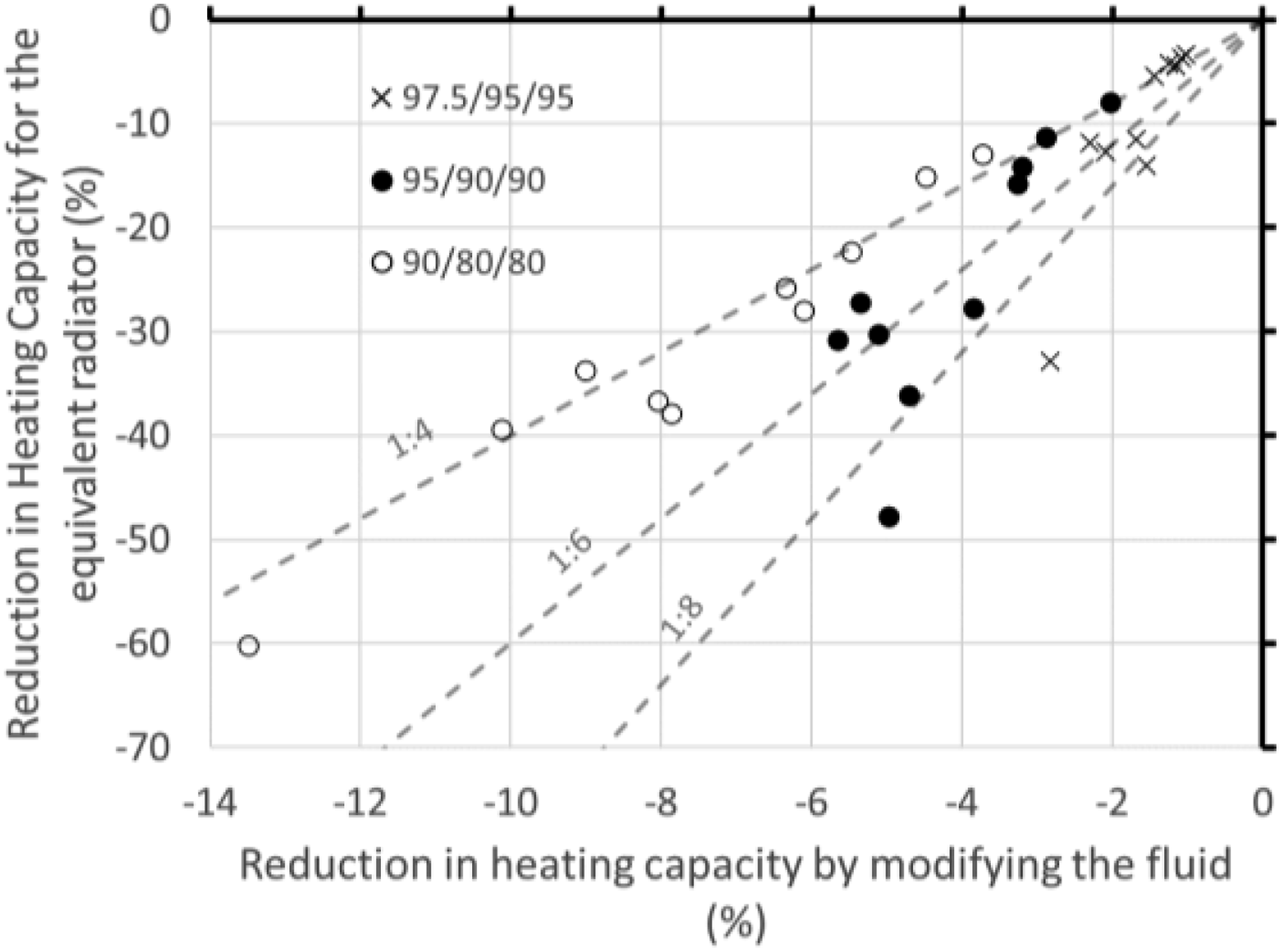

Conclusions

Analysis has been carried out across a range of reasonable building room scenarios. Cycle energy reduced by between 5 and 25%, and cycle mean power by between 0 and 7% depending on the particular scenario. This work has shown that:

1. A significant opportunity exists to deliver comfortable space heating with reduced energy input by changing the fluid properties, in particular, the fluid specific heat capacity and those which impact on the mass flow rates through the radiator;

2. Water side thermal resistance in isolation was shown to have a negligible effect on the mean heating power, but can have a positive effect on the individual cycle energy;

3. The opportunity for energy savings tends towards the reduction in individual cycle energy when the heating event is of a duration equivalent to or smaller than the individual cycle duration;

4. Scenarios with a lower heat flow ratio, indicating, for example, better levels of room insulation or larger heat emitters, showed more opportunity for energy saving;

5. Achieving these savings by changing fluid properties has a smaller impact on the ability of the heating system to cope with extreme cold conditions than achieving the same energy saving by reducing the radiator size.

Supplemental Material

Supplemental Material - Opportunities for improved space heating energy efficiency from fluid property modifications

Supplemental Material for Opportunities for improved space heating energy efficiency from fluid property modifications by Andy M Williams and Daniel T Innerdale in Indoor and Built Environment.

Footnotes

Acknowledgements

The authors would like to acknowledge the support from Endo Enterprises (UK) Ltd and the UK Higher Education Innovation Fund (HEIF) who funded the research. The authors acknowledge the support from Liverpool John Moores University through their Cheshire and Warrington 4.0 project from which the experimental validation data was provided.

Author contributions

The underlying work was done by Dr Andy Williams with support from Mr Daniel Innerdale.

Declaration of conflicts interest

The author(s) declared the following potential conflicts of interest with respect to the research, authorship, and/or publication of this article: Dr A.M. Williams is employed by Endo Enterprises (UK) Ltd.

Funding

The author(s) disclosed receipt of the following financial support for the research, authorship, and/or publication of this article: This work was supported by Endo Enterprises (UK) Ltd, the UK Higher Education Innovation Fund and the European Regional Development Fund, through the Cheshire and Warrington 4.0 project.

ORCID iD

A.M. Williams

Supplemental Material

Supplemental material for this article is available online.

References

Department for Business,; Energy & Industrial Strategy . Energy Consumption in the UK 2021. London: Report HMSO, 2021.

Tamas

Ouf

O’Brien

. A field study on the effect of building automation on perceived comfort and control in institutional buildings. Architectural Sci Rev 2020; 63: 74–86.

ONS . CT0823 – Number of Bedrooms by Type of Central Heating, Data from Census. London, 2018. as presented by Office for National Statistics.

Munton

Wright

Mallaburn

Boait

. How Heating Controls Affect Domestic Energy Demand: A Rapid Evidence Assessment. A Report to the Department of Energy and Climate Change. London: DECC, 2014.

Huang

Katipamula

Lutes

. Experimental investigation on thermal inertia characterization of commercial buildings for demand response. Energy and Buildings 2021; 252: 111384.

Peet

. Effect of an on/off HVAC control on indoor temperature distribution and cycle variability in a single-floor residential building. Energy and Buildings 2021; 251: 111289.

Alhashme

Ashgriz

. A virtual thermostat for local temperature control. Energy and Buildings 2016; 126: 323–339.

Lee

Heo

. Simplified data-driven models for model predictive control of residential buildings. Energy and Buildings 2022; 265: 112067.

Chen

Feng

. Model predictive control optimization for rapid response and energy efficiency based on the state-space model of a radiant floor heating system. Energy and Buildings 2021; 238: 110832.

10.

Gupta

Badr

Negahban

Qiu

. Energy-efficient heating control for smart buildings with deep reinforcement learning. J Building Eng 2021; 34: 101739.

11.

Huchuck

Sanner

O’Brien

. Development and evaluation of data-driven controls for residential smart thermostats. Energy & Buildings 2021; 249: 111201.

12.

BRE . Wet Central Heating Systems: Treatment of Heat Transfer Modifiers, Inhibitors, Flushing Techniques and Inline Cleaners in the National Calculation Methodology for Energy Rating of Dwellings (SAP). BRE, Garston,: SAP Principle Paper V1.2, 2014.

13.

Keklikcioglu

Ozceyhan

. Heat transfer augmentation in a tube with conical wire coils using a mixture of ethylene glycol/water as a fluid. Int J Therm Sci 2022; 171: 107204.

14.

Tsukahara

Kawase

Kawaguchi

. Heat transfer in a viscoelastic orifice flow at low to moderate Reynolds numbers. Comput Therm Sci 2014; 6: 79–90.

15.

Tsukahara

Hara

Kawada

Kawaguchi

. Experimental study on functionality of surfactant solution in turbulent heat transfer by varying local shear rate. Int J Heat Mass Transfer 2016; 102: 360–368.

16.

Wang

Zakin

Shi

. Review on Drag Reduction and Its Heat Transfer by Additives. Adv Mech Eng 2011; 3: 478749.

17.

Guo

Surblys

Kawagoe

Matsubara

Liu

Ohara

. A molecular dynamics study on the effect of surfactant adsorption on heat transfer at a solid-liquid interface. Int J Heat Mass Transfer 2019; 135: 115–123.

18.

Sholahudin

Ohno K

Ohno

Giannetti

Yamaguchi

Saito

Dynamic modeling of room temperature and thermodynamic efficiency for direct expansion air conditioning systems using Bayesian neural network. Appl Therm Eng 2019; 158: 113809.

19.

Thilker

Bacher

Cali

Madsen

. Identification of non-linear autoregressive models with exogenous inputs for room air temperature modelling. Energy and AI 2022; 9: 100165.

20.

Liu

Zhang

Wang

Song

You

Jiang

A thermal-hydraulic coupled simulation approach for the temperature and flow rate control strategy evaluation of the multi-room radiator heating system. Energy 2022; 246: 123347.

21.

Vivian

Croci

Zarrella

. Experimental tests on the performance of an economic model predictive control system in a lightweight building. Appl Therm Eng 2022; 213: 118693.

22.

Thilker

Bacher

Bergsteinsson

Junker

Cali

Madsen

. Non-linear grey-box modelling for heat dynamics of buildings. Energy and Buildings 2021; 252: 111457.

23.

. Dynamic simulation of space heating systems with radiators controlled by TRVs in buildings. Energy and Buildings 2008; 40: 1755–1764.

24.

Ahn

B-C

Song

J-Y

. Control characteristics and heating performance analysis of automatic thermostatic valves for radiant slab heating system in residential apartments. Energy 2010; 35: 1615–1624.

25.

Ruivo

Ferreira

Vaz

. Prediction of thermal load temperature difference values for the external envelope of rooms with setback and setup thermostats. Appl Therm Eng 2013; 51: 980–987.

26.

Stelrad Radiator Group , Savanna I Compact. Product Datasheet, accessed January 2022.

27.

Seifert

Knorr

Meinzenbach

Bitter

Gregersen

Krogh

. "Review of thermostatic control valves in the European standardization system of the EN 15316-2/EN 215". Energy and Buildings 2016; 125: 55–65.

Supplementary Material

Please find the following supplemental material available below.

For Open Access articles published under a Creative Commons License, all supplemental material carries the same license as the article it is associated with.

For non-Open Access articles published, all supplemental material carries a non-exclusive license, and permission requests for re-use of supplemental material or any part of supplemental material shall be sent directly to the copyright owner as specified in the copyright notice associated with the article.

0.00 MB

0.37 MB