Understanding lifetime and dispersion of cough-emitted droplets in air

Abstract

To understand the exact transmission routes of SARS-CoV-2 and to explore effects of time, space and indoor environment on the dynamics of droplets and aerosols, rigorous testing and observation must be conducted. In the current work, the spatial and temporal dispersions of aerosol droplets from a simulated cough were comprehensively examined over a long duration (70 min). An artificial cough generator was constructed to generate reliably repeatable respiratory ejecta. The measurements were performed at different locations in front (along the axial direction and off-axis) and behind the source in a sealed experimental enclosure. Aerosols of 0.3–10 µm (around 20% of the maximum nuclei count) were shown to persist for a very long time in a still environment, and this has a substantial implication for airborne disease transmission. The experiments demonstrated that a ventilation system could reduce the total aerosol volume and the droplet lifetime significantly. To explain the experimental observations in more detail and to understand the droplet in-air behaviour at various ambient temperatures and relative humidity, numerical simulations were performed using the Eulerian–Lagrangian approach. The simulations show that many of the small droplets remain suspended in the air over time instead of falling to the ground.

Introduction

The coronavirus disease (COVID-19) pandemic demonstrated the importance of research in understanding disease transmission to limit the spread of infectious pathogens and prevent future pandemics. The novel coronavirus (SARS-CoV-2) spreads infection mainly through respiratory droplets.^1–4 In the early stages of a pandemic, usually no effective vaccine or medication is available; therefore, preventive measures should be taken seriously to prevent transmission. During the H1N1 influenza pandemic in 2009, the utilization of face coverings such as N95 respirators and surgical and non-surgical (fabric) masks was recognized to be an effective method to reduce the contraction of infectious droplets.^5–7 Similarly, the effectiveness of using masks against SARS-CoV-2 was once again refreshed and supplemented by recent studies, which firmly established the importance for the general public to wear non-surgical masks for community safety.^8–10 A successful public health program hinges on whether all disease transmission mechanisms are prevented. There is a need for a better understanding of airborne disease transmission to develop effective personal protective equipment (PPE) and inform the public on best practices.

The SARS-CoV-2 virus (diameter ∼0.1 μm) is carried in respiratory droplets (diameter ∼0.2 μm to several mm). ¹¹ The virus can be transmitted from an infected person to a healthy one via (a) exposure to environmental fomites; (b) close contact with virus-carrying droplets; and/or (c) aerosol transmission, that is, inhalation of very small droplets. The decision on the type of PPE to use is based on the risk of whether the particles produced are of airborne size (≤ 5 μm) or droplet size (> 5 μm). ¹² The cut-off size of 5 µm is approximate because the droplets become gradually more airborne as the aerodynamic diameter is reduced, and as a result, different cut-off diameters were postulated.^13–15 The virus is most frequently transmitted at short distances, that is, within the projectile range of droplets. Outside the 2-m range, the occurrence of droplets is generally believed to be rare as the gravitational settling is more potent than diffusion. In contrast, aerosols stay airborne longer and thus, have a higher transmission risk, requiring more expensive and elusive PPE, such as N95/P100 masks. In a recent article, Inthavong ¹⁶ showed that airborne particles that move within the breathing zone enter the nostrils. Inside the nasal cavity, micron and submicron particles were found and these can be deposited in very different ways (inertial impaction, sedimentation and diffusion) and at various positions. From particulate matter research, particles with effective aerodynamic parameters of less than 2.5 µm (PM_2.5) are known to penetrate deep into the lungs.^17–19 Consequently, small aerosol nuclei can carry the virus deeper into the respiratory tract

The higher incidence of source-proximate transmissions is often used to advocate for the dominance of transmissions by fomites and droplets; however, an alternative explanation based on aerosol transmission can be postulated that aerosol transmission efficacy is weakened with the square of the distance from the source due to dilution. Nevertheless, the aerosol route is the primary mechanism for transmissions spatially and temporally far from the point of source.^20–27 The SARS-CoV-2 virus can remain active in aerosols for over 3 h depending on the UV index, temperature and relative humidity (RH).^3,28–32 To find the stability of SARS-CoV-2 in aerosols and estimate the airborne decay rate, several studies have been conducted. For instance, in the work of Dabisch et al., ³⁰ a rotating drum aerosol chamber was designed to analyse the effect of temperature, sunlight and RH on the persistence of SARS-CoV-2 in aerosols. Aerosols with a mass median aerodynamic diameter (MMAD) of 2 μm were generated and injected into the chamber for 20–30 s to achieve a quantifiable concentration of infectious virus. While the results of this study were significant in terms of estimating the aerosol lifetime as a function of environmental conditions, the scope of the work was limited to a single particle size distribution with a specific MMAD. However, a wide range of particle size distributions is possible depending on the type of respiratory event and the individual. As discussed in their paper, ³⁰ the droplet size has the potential to change their results significantly.

Other factors, in addition to the survival of virus in aerosols and droplet size, can affect aerosol transmission of disease and, therefore, also need to be taken into account in any evaluation of the influence of ambient conditions on transmission. Some of these factors are the size distribution, the viral load of droplets shed from infected people, the amount of virus required to transmit the disease via aspiration and the proximity of people and airflow properties within a given space. For example, droplet dynamics depend on the flow regime, that is, whether turbulent eddies exist, and their intensity. Inthavong ¹⁶ showed a broad range of complicated flow regimes including recirculation, Coanda flow, separation and reattachment can be generated in the indoor environment. When the air current velocities are large enough and circulation zones exist, droplets larger than 5 µm can easily be trapped within the air currents and travel long distances.^33–35 This mechanism was implicated in the analysis of a restaurant transmission case where the air-conditioning currents were believed to transport the droplets. ³⁶ These cases cast doubt on the validity of the 2-m distancing measure. Liu et al. ³⁷ also showed that the 2-m physical distancing rule may enhance transmission risk in a stratified environment. Unfortunately, at the moment, a complete dataset or model including the effects of all the main factors stated above have not yet been reported.

At the present time, the airborne disease transmission is of particular interest as several nations ramp-up vaccine rollout and initiated a return-to-normal protocol. As office spaces are re-populated and limitations on public gatherings are lifted, the aerosol transmission mechanism can become the dominant one. Physical distancing and hygiene measures are much less effective at preventing airborne transmission. Instead, more costly infrastructural changes such as redesign of HVAC systems are required. ³⁸ This necessitates a more complete understanding of respiratory ejecta and aerosol dynamics.

There are several studies on respiratory ejecta using sampling^39,40 and optical methods, for example, particle image velocimetry (PIV),^41,42 schlieren photography^43,44 and MIE scattering. ⁴⁵ Yang et al. ⁴⁰ compared cough with and without a P100 mask and found that the size distribution of cough nuclei was multimodal with most of the droplets within the 0.7–2.1 µm range. To prevent sampling errors, Chao et al. ⁴¹ performed laser-based experiments on human respiratory ejecta. The PIV and MIE scattering techniques were used to obtain the velocity vector fields and droplet size distributions, respectively. The average exhalation air velocity was about 12 and 4 m/s for coughing and speaking, respectively. The droplet size distribution also depended on the type of the respiratory event with mean diameters greater than 10 µm. However, the optical measurement technique utilized had a low sensitivity limit of 2 µm. When techniques that can measure submicron droplets are used, findings suggest that there are more droplets generated in the aerosol range.^46,47

Liu and Novoselac ⁴⁸ studied the dispersion of a simulated cough and measured particle trajectories for particle sizes of 0.77, 2.5 and 7 µm. They found that 7-µm particles settled within the 2-m range, 2.5-µm particle trajectories were affected by gravity, and 0.77-µm particles were completely suspended. Stadnytskyi et al. ¹ measured the time history of laser light scattered off airborne droplets in the wake of speech into a container. The data were binned into two intensity levels with no association to droplet sizes. The droplets with higher scattered light intensity had shorter lifetimes with an exponential decay time constant of 8 min in comparison to 14 min of droplets with dimmer scattering light intensity.

There is still a lack of benchmark data documenting the spatial and temporal dispersion of aerosol droplets at different sizes over a long duration (70 min). In fact, in the present study, the effects of droplet size distribution, the airflow characteristics and the distance from the cough source on the decay rate and aerosol persistence were investigated. This data would be very useful to validate numerical and theoretical studies. Additionally, there is a practical and clinical need to quantify how different aerosol sizes disperse. To that end, for the present study, an artificial cough generator was built that can produce repeatable respiratory ejecta with user-defined parameters. Aerosol dispersions at various size bins within 0.3–10+ µm were measured at different locations. A very long sampling duration of over 1 h was chosen in order to capture the complete gravitational sedimentation of the aerosol plume.

Detailed numerical simulations have been performed to show the droplet trajectories and patterns across different relative humidities and temperatures, to understand and discuss the physical phenomena behind the experimental observations. From a fluid mechanics point of view, the human cough can be considered as a multiphase incompressible buoyant turbulent flow. ³⁴ In general, the cough flow depends on human physiology, and its transport characteristics can be affected by several parameters such as the mouth opening area, the unsteady flow rate, the jet flow direction, as well as the ambient conditions such as the temperature and RH. ⁴⁹

Numerous numerical simulations have been performed to investigate the effects of different parameters on the coughing phenomenon. In general, two different methods, known as the Eulerian–Lagrangian (EL) approach and the Eulerian–Eulerian (EE) approach, have been utilized to model the gas-particle two-phase flows in indoor environments.^50–57 In these approaches, the gas flow is simulated using the Navier–Stokes equations, but the particle movement is modelled differently. In the EL approach, the particles are tracked individually through the air using the particle dynamic equations (by considering the drag force, buoyancy force, etc.) and, therefore, the particle trajectories can be directly predicted. However, to predict the particle concentration, additional post-processing is needed. By contrast, in the EE approach, the dispersed particles are modelled as a continuous phase. Using this approach, the particle concentration can be obtained directly, whilst it cannot predict the particle trajectories. ⁵⁷ Since the particles are considered as a continuous phase in this approach, simulating the particle–wall interaction and bouncing behaviour is also challenging.

In a recent study, Yan et al. ⁵⁷ investigated the behaviour of micron-sized particles in a displacement ventilated room using both the EE and the EL approaches. In their work, the EE two-fluid model was used, where one set of conservation equations was solved for each phase. To model the particle–wall interaction in the EE model, a free-slip boundary condition was implemented at the solid walls as an approximation. Both EE and EL models predict very similar gas flow fields. In addition, the overall distribution patterns of the particles predicted by these models are very close. However, the authors showed that although different post-processing techniques such as the sampling volume method and the kernel method have been developed so far to convert particle trajectories into particle concentration in the EL approach,^58,59 the accuracy and stability of these methods are still not satisfactory. ⁵⁷ In addition, they demonstrated that the EE model actually fails to mechanistically simulate the particle–wall interactions. In the present study, the EL approach was used to model the cough flow due to the low concentration of droplets and the interest in finding the particle trajectory.

Methodology

Experimental methodology

There are a few respiratory event simulators in the literature; some utilize pressurized air,^48,60,61 and others mechanical systems, ⁶² to drive the cough. A novel artificial ‘cough’ generator that produces spray, emulating from a cough, sneeze or speech, was constructed, as shown in Figure 1. The system consists of flow lines and controllers, solenoid and manual valves, an aerosol generator, a HEPA filter, a control box, a digital delay generator and an airway manikin.

Figure 1.

Schematic of the respiratory ejecta simulator and the control electronics.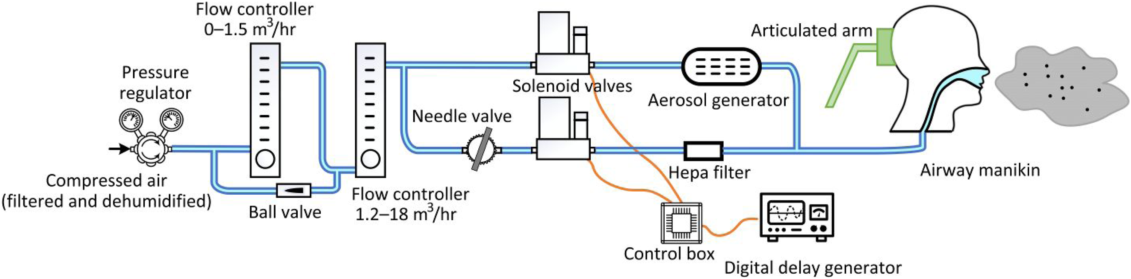

Filtered and dehumidified air is regulated to a constant pressure. The flow rate of the cough, hence the cough velocity, was calibrated using two variable area flowmeters/controllers (Omega FL-2010: 0–1.5 m³/h range, and Omega FL-2064: 1.2–18 m³/h range). For the experiments presented in this study, the cough generator was calibrated to produce coughs at a maximum flow rate of 3 m³/h through the flow controller. The resulting cough average velocity through the manikin mouth was calculated as 4.8 m/s. The flow was then separated into two lines, that is, the aerosol and by-pass lines. Each line incorporates a solenoid valve (ASCO/Emerson brand) to control the flow duration. A control box was designed and built in-house which converts a 0‒5 VDC control signal from the digital delay generator (Berkeley Nucleonics, model 577) to a 110-VAC power output to control the solenoid valves. This digital delay generator allows for eight independently controlled signal outputs of user-defined width (10 ns–1000 s). These signals were used to control the cough duration and timing. The choice of electronic control also allows for cough synchronization with camera systems and laser/LED-based lighting. The droplet generation was done by a polydisperse aerosol generator (LaVision brand) employing a Laskin-type nozzle. A propylene glycol solution was atomized at a droplet production rate of over 10⁸ particles per second. This solution was chosen because high concentrations of droplets can be generated using a Laskin nozzle; the droplet sizes are polydisperse and within the size range of interest; and the fluid is non-toxic. The droplet loading can be calibrated by monitoring the outlet via the droplet generator and by adjusting the bypass flow rates via a needle valve connected to the bypass flow line. The droplet size distribution was adjusted via changing a pressure regulator on the nozzle. The droplet size distribution obtained from the aerosol generator is given in Table 1 and Figure 2. The aerosol-laden flow was released from an airway manikin. The orientation and height of the manikin head were adjusted using an articulated arm. This setup was capable of generating repeatable respiratory ejecta with controlled cough flow rates, duration and timing. This flexibility is crucial for future studies because cough properties depend on several parameters. For example, cough flow rate and temporal profile have a high variance among individuals and depend on characteristics such as age and gender.^49,63

Table 1.

Droplet size distribution at the aerosol generator exit.

Droplet sizes	Concentration
Total	> 108 #/cm3
0.2 μm	2 × 107 #/cm3
0.5 μm	5 × 107 #/cm3
1.0 μm	1 × 103 #/cm3
0.3–0.5 μm	1.5 × 107 #/cm3
0.5–1.0 μm	8 × 106 #/cm3
Modal	0.25 μm

Figure 2.

The droplet size distribution obtained from the aerosol generator.

A commercial particle counter (Kanomax brand), with a calibration traceable to NIST, was used to collect samples from various locations within the chamber. The counter is capable of measuring concentrations in 6 bin sizes of 0.3, 0.5, 1.0, 3.0, 5.0 and 10.0+ µm. The particle counter operates at the sampling rate of 0.14 Hz. A sampling collection time of over 1 h was performed for each experimental run.

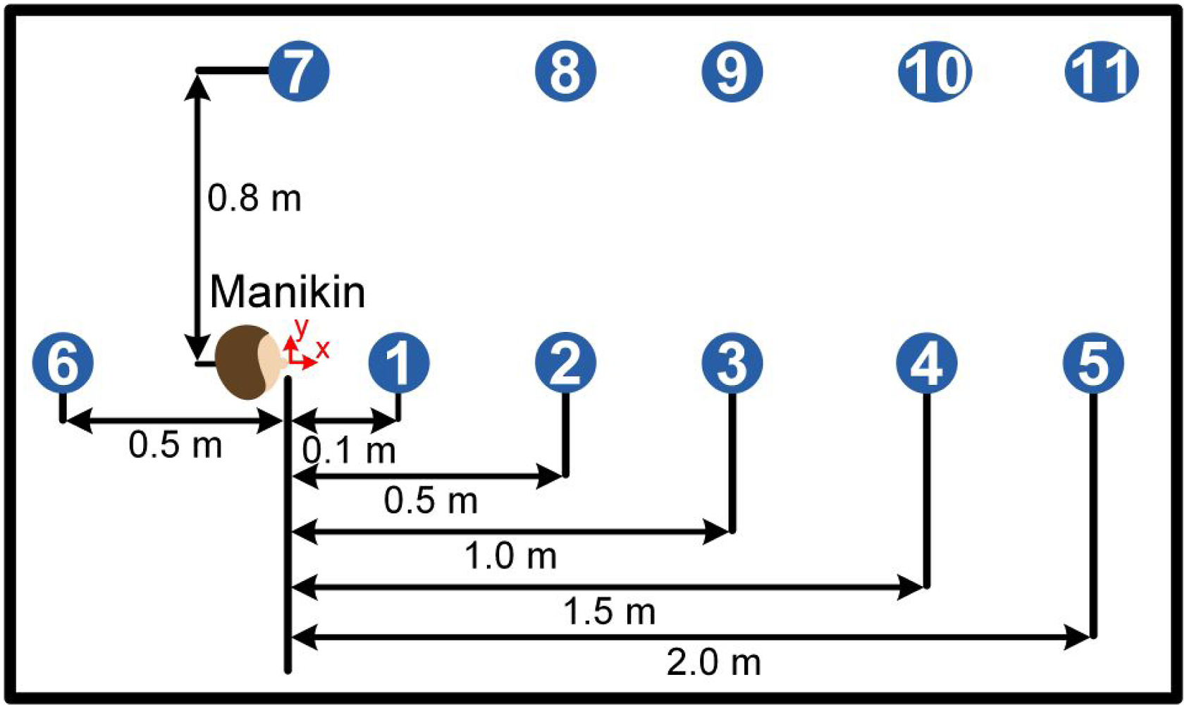
A sealed experimental enclosure was built with dimensions of 2.5 m long, 1.6 m wide and 1.9 m in height. The manikin was placed within the chamber on an articulated arm, with the mouth located at a height of 1 m. Figure 3 shows the experimental enclosure as well as the manikin used in the present study. The cough flow tubing leaving the chamber was connected to the remainder of the particle-generating system. The particle counter was attached to a tripod and adjusted to a height where the sampling intake was at the height of the manikin’s mouth. Eleven locations were tested using the particle counter, as shown in Figure 4. Locations 1 through 5 were located along the direction of the cough, in 0.5-m intervals, with the exception of location 1, which was 0.1 m in front of the mouth. Location 6 was placed 0.5 m behind the mouth, in the opposite direction of the cough. Locations 7 through 11 were located 0.8 m to the side of the mouth, again in 0.5-m intervals in the direction of the cough. The enclosure was attached to a vent system which was engaged between experiments to vent the enclosure.

Figure 3.

The sealed experimental enclosure and the manikin.

Figure 4.

A schematic of the cough chamber and the measurement locations in relation to the manikin.

The experimental procedure was initiated by triggering 5 consecutive coughs to ensure proper flow through the system. The enclosure was then vented for 15 min before continuing to the main procedure, and the particle counter was purged for internal cleaning using the instrument’s zero filter. For each test, the particle counter was set to sample at 7-s intervals for a total of 620 intervals, totalling a sampling time of 72 min. After the particle counter was manually triggered to start the experiment, the enclosure was sealed and the cough was triggered using the digital delay generator at the 20th time interval. The particle counter was then run for the following 600 seven-second intervals of the experiment, measuring the particles at the location under investigation. After each experiment was completed, the enclosure was vented for 5 min and the particle counter was purged during this time using an inlet filter. The background levels were measured in the 5 mins preceding the cough measurements, and the base reading was subtracted from the cough droplet reading. Although a correction was applied, the background levels were several orders of magnitude smaller than the cough readings as a high concentration of droplets were generated with the particle generator. The humidity and temperature within the enclosure were recorded for each day of experiments, as shown in Table 2. The experimental setup lacked climate control capabilities, and as a result, experimental data from different locations corresponded to different temperatures within a range of 21.9–25.8°C. The humidity varied from 20 to 78%. A total of 55 experiments were performed; 5 measurements at 11 sampling locations.

Table 2.

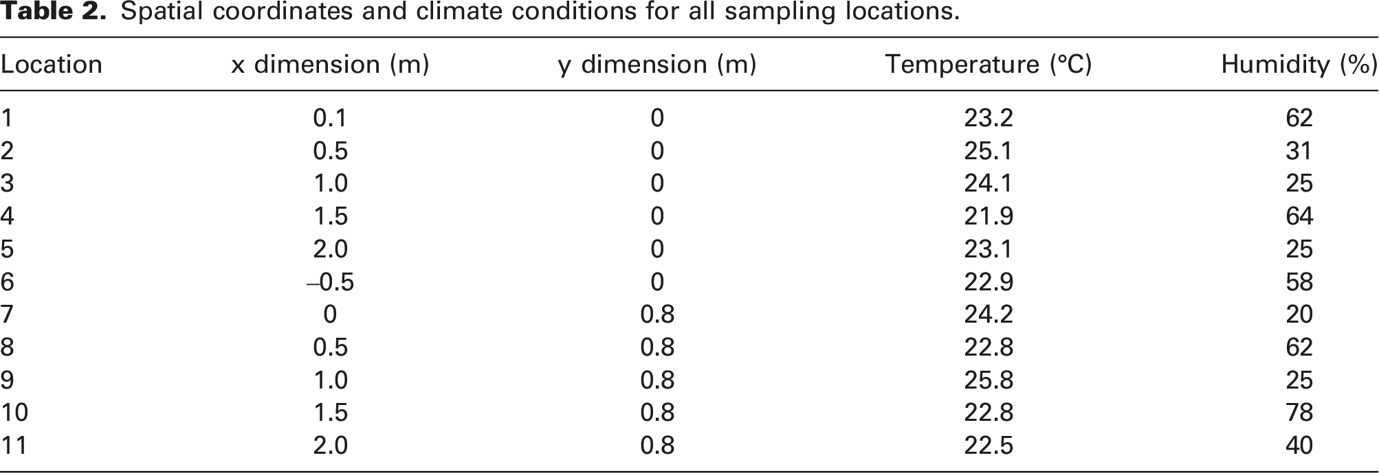
Spatial coordinates and climate conditions for all sampling locations.

Location	x dimension (m)	y dimension (m)	Temperature (°C)	Humidity (%)
1	0.1	0	23.2	62
2	0.5	0	25.1	31
3	1.0	0	24.1	25
4	1.5	0	21.9	64
5	2.0	0	23.1	25
6	‒0.5	0	22.9	58
7	0	0.8	24.2	20
8	0.5	0.8	22.8	62
9	1.0	0.8	25.8	25
10	1.5	0.8	22.8	78
11	2.0	0.8	22.5	40

Numerical methodology

In the present work, the Eulerian–Lagrangian approach was utilized to simulate the cough flow. Ansys ^® Academic Fluent (Release 2020 R2) software was utilized to perform the simulations. The mass, momentum, energy and species equations were discretized based on the finite volume method. As shown in Figure 5, the computational domain consists of a circular orifice with a diameter of 0.0217 m, which was located 0.72 m above the ground on the left side of a 1.81 m by 1.81 m square domain (used to represent a closed room). In fact, the orifice diameter was equal to the typical human mouth diameter at the time of coughing. ⁴⁹ The adiabatic no-slip boundary condition was used for the walls as shown in Figure 5.

Figure 5.

Visual of computational domain size and meshing used in numerical simulations.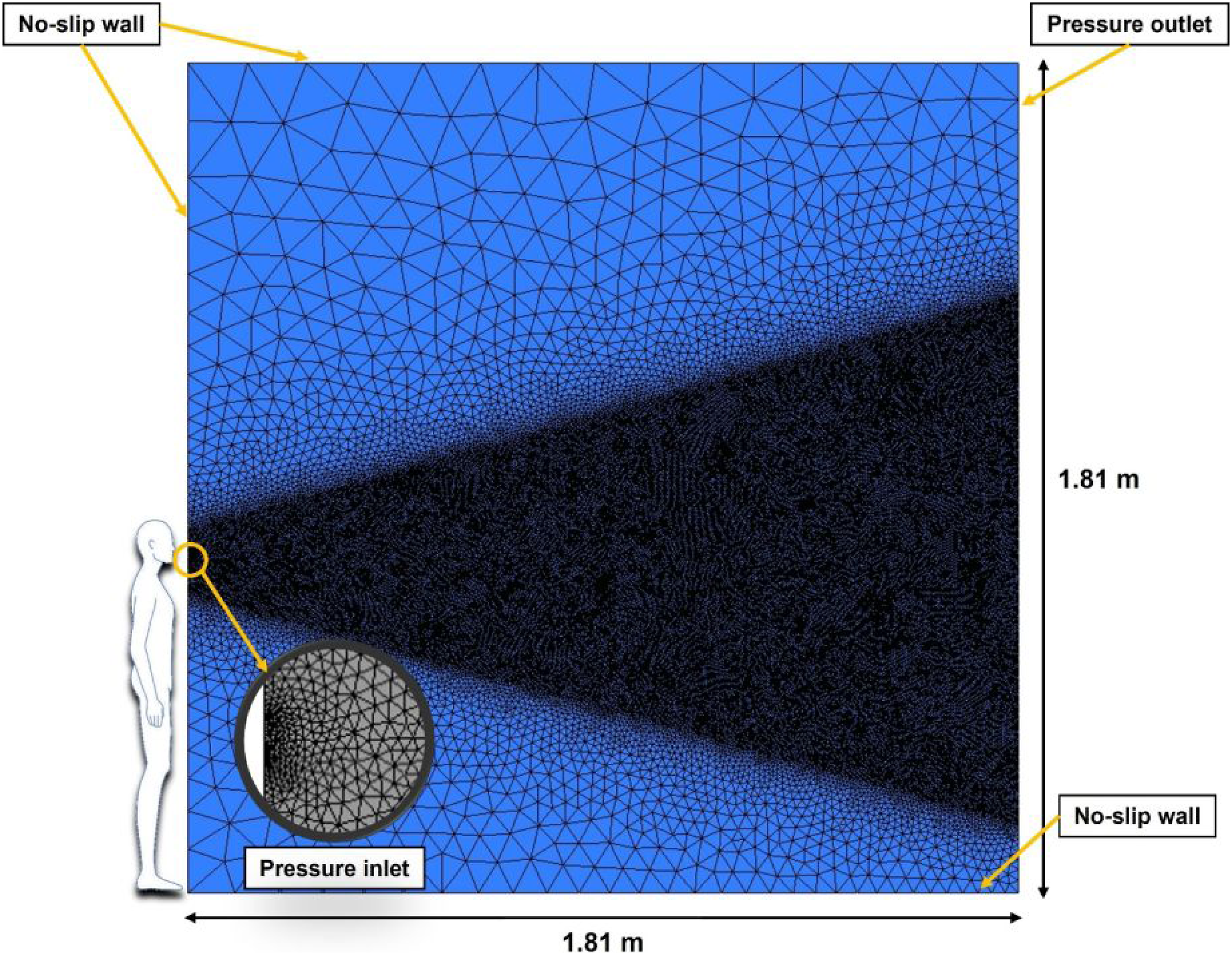

As shown in Figure 5, the mesh near the orifice and in the cone region is much finer than that in the far regions. The cell size used was approximately 80 μm near the orifice. This non-uniform mesh structure is important to capture the flow field of coughing accurately and to reduce the computational cost. Inside the cone region, the air velocity and velocity gradients are high. Therefore, a very fine mesh is necessary to capture these details.

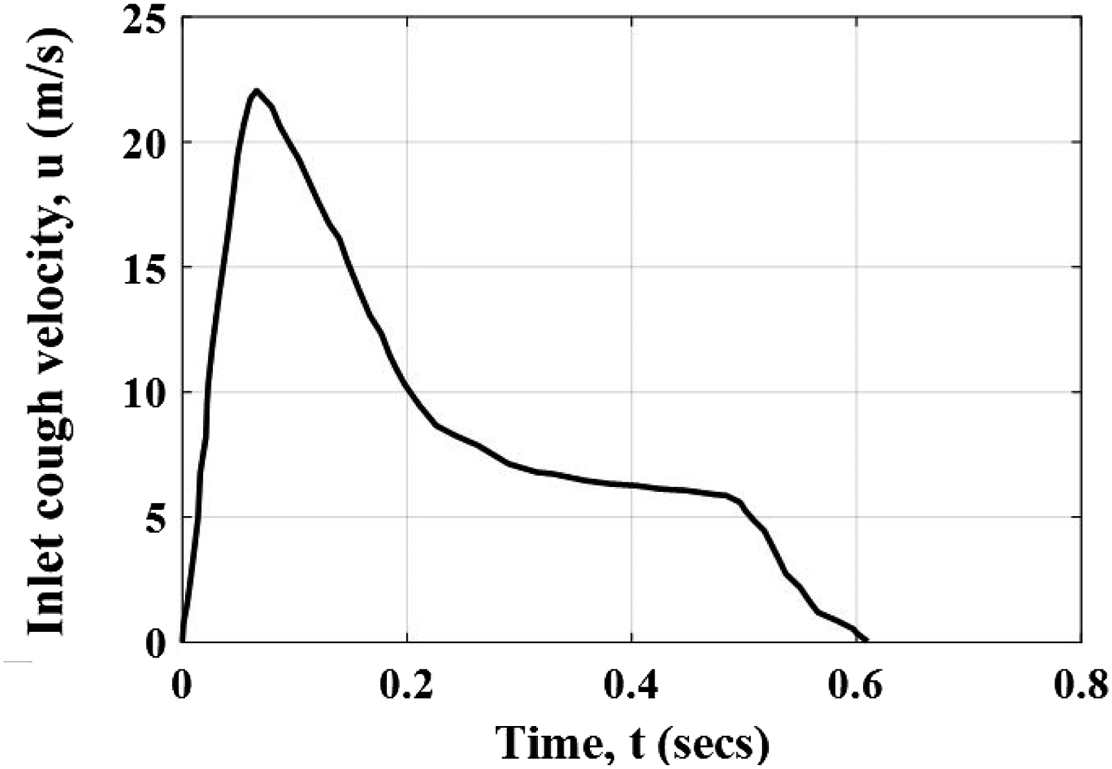
At the orifice, a transient velocity profile, which represents the unsteady velocity of the cough at the human mouth, was imposed as the inlet boundary condition for the airflow. The velocity profile was obtained from the experimental work of Gupta et al. ⁴⁹ and is shown in Figure 6. As can be seen, the velocity reached its maximum value (around 22 m/s) at 0.066 s, and the whole process would take about 0.61 s. Since the expired flows might be affected by the temperature and buoyancy, based on Zhu et al., ⁶⁴ the air temperature at the orifice was fixed at 32°C. To study the effect of ambient conditions on the droplet behaviour, different temperatures and relative humidities were considered in the current work. The ambient temperatures and relative humidities tested were 18°C, 21°C and 25°C, and 30%, 50% and 80%, respectively. The velocity of the ambient air was set to zero as the initial condition.

Figure 6.

Inlet velocity for the airflow (adapted from Gupta et al. ⁴⁹ ).

In the present work, the shear stress transport (SST) k-ω turbulence model was utilized.^65,66 To solve the turbulence of the continuous phase, the standard k-ε, the renormalization group (RNG) k-ε, the standard k-ω and the SST k-ω have all been widely used in the literature. However, the previous studies showed that the RNG k-ε and the SST k-ω models are able to successfully predict the major details of coughing with a reasonable computational cost.^67,68

The coupled scheme was used for pressure–velocity coupling. In this algorithm, the momentum and the pressure-based continuity equations were solved together. According to Ansys ^® Fluent 12.0 User’s Guide, ⁶⁹ the coupled algorithm has a better performance in terms of robustness and accuracy compared to the segregated solution schemes. In addition, for the pressure interpolation, the PRESTO! (PREssure STaggering Option) scheme was applied. For the gradient terms, the Green–Gauss node-based scheme was applied. This algorithm is generally more accurate than the cell-based schemes, especially for unstructured meshes. ⁶⁹ In addition, the second-order upwind scheme was used to spatially discretize the momentum, energy and species equations. For the temporal discretization, the bounded second-order implicit technique was used. Based on the Courant–Friedrichs–Lewy limit, the time step was fixed at 0.135 ms in this study. ⁷⁰

In the present work, evaporative pure-water droplets were injected into the computational domain through the orifice (adding non-evaporative materials is the subject of future works). A wide range of droplet sizes was considered in this study since the size distribution obtained from coughing is not unique and depends on human physiology. Here, the droplet sizes ranged from 3 to 750 μm, and the Rosin–Rammler function with the spread parameter value of 4 was used to estimate the size distribution. ⁷¹ The group injection type with 10 streams (i.e. the droplets were grouped into 10 sizes) was used to inject the droplets. Based on the work of Bi, ⁶⁸ the total mass flow rate of the discrete phase was 7.44 g/s. The mass flow rate and droplet concentration strongly depend on human physiology. For instance, Yang et al. ⁴⁰ found that the average droplet concentration for males is considerably greater than that for females because males typically have a longer cough flow rate than females. Furthermore, they showed that people in the 30- to 50-year-old age group have the highest droplet concentrations, since they have the longest cough flow rate. In the present work, similar to the study of Bi, ⁶⁸ the droplet injection started at 0.042 s and stopped at 0.136 s. This time period corresponds to the duration that spans the peak velocity of the cough (see Figure 5).

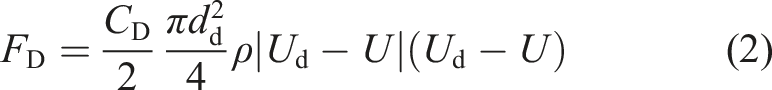
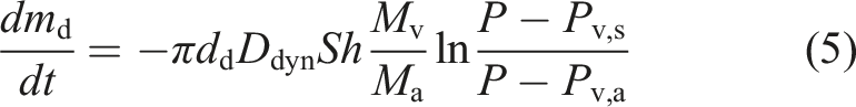
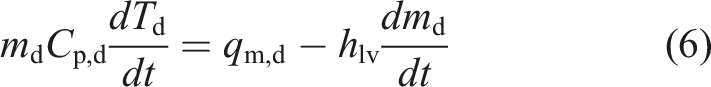
To predict the droplet trajectory, velocity and temperature at different time steps, the Lagrangian discrete phase model was used. The force balance equation (equation (1)), which was based on Newton’s second law of motion, equates the summation of drag 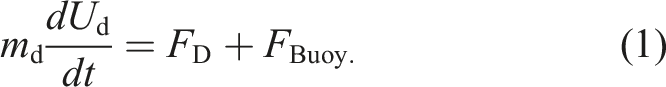$\left(F_D\right)$ (equation (2)) and buoyance $\left(F_{Buoy.}\right)$ forces (equation (3)) with the droplet inertia

$m_{\text{d}}\frac{d{U}_{\text{d}}}{dt}=F_{\text{D}}+F_{\text{Buoy}.}$

(1)

$F_{\text{D}}=\frac{C_{\text{D}}}{2}\frac{\pi d_{\text{d}}^2}{4}\rho \left|U_{\text{d}}-U\right|\left(U_{\text{d}}-U\right)$

(2)

$F_{\text{Buoy}.}=\frac{\pi d_{\text{d}}^3}{6}\left({\rho }_{\text{d}}-\rho \right)g$

(3)

where $m_{\text{d}}$ , $U_{\text{d}}$ , $d_{\text{d}}$ , ${\rho }_{\text{d}}$ and $C_{\text{D}}$ are the droplet mass, velocity, diameter, density and drag coefficient, respectively. ⁷² Moreover, $U$ , $\rho$ and $g$ are the gas velocity, density and the gravitational acceleration, respectively. Since the Reynolds number, Re, is relatively low and the flow is incompressible in the present study, the spherical drag coefficient, as defined by equation (4), is employed

$C_{\text{D}}=a_1+\frac{a_2}{Re}+\frac{a_3}{R{e}^2}$

(4)

where $a_1$ , $a_2$ and $a_3$ are constants. ⁷³ In addition, the droplet breakup phenomenon was considered by using the Taylor analogy breakup (TAB) model. The TAB model was based on an analogy between an oscillating and distorting droplet and a spring-mass system, which is suitable for low Weber number flows.^69,74 Although this model was included in the simulations, the results showed that almost no breakup happened during the droplet transport. Therefore, modelling the breakup phenomenon could be generally ignored. To model the droplet coalescence, a stochastic collision model (which is based on O’Rourke’s algorithm) was used.^69,75 In addition, a two-way turbulence coupling between the continuous and discrete phases was considered. Similar to the study of Yan et al., ⁷² the evaporation was assumed to be controlled by the equilibrium vapour pressure relative to the ambient pressure at the droplet surface. For the droplets suspended in the air, the diffusion mechanism and the mass flow rate dominate the evaporation, as described by equation (5)

$\frac{d{m}_{\text{d}}}{dt}=-\pi d_{\text{d}}{D}_{\text{dyn}}Sh\frac{M_{\text{v}}}{M_{\text{a}}}\text{ln}\frac{P-P_{\text{v},\text{s}}}{P-P_{\text{v},\text{a}}}$

(5)

where $t$ is time, $D_{\text{dyn}}$ is the dynamic diffusivity of water vapour in the air, $Sh$ is the Sherwood number, $M_{\text{v}}$ is the molecular weight of the vapour, $M_{\text{a}}$ is the molecular weight of the mixed air, $P$ is the ambient pressure, $P_{\text{v},\text{s}}$ is the partial vapour pressure at the droplet surface and $P_{v,a}$ is the partial vapour pressure in the air. Like other studies in this field,^57,68,72 in the present work, the temperature gradient inside a droplet was ignored and the lumped capacity method was used to model the droplet temperature and heat transfer, as described by equation (6)

$m_{\text{d}}{C}_{\text{p},\text{d}}\frac{d{T}_{\text{d}}}{dt}=q_{\text{m},\text{d}}-h_{\text{lv}}\frac{d{m}_{\text{d}}}{dt}$

(6)

where $q_{\text{m},\text{d}}$ is the interfacial rate of heat transfer and $h_{\text{lv}}$ is the latent heat of vaporization. In the current work, the Nusselt and Sherwood number correlations developed by Ranz and Marshall were used.^76,77 Moreover, to solve the force balance and heat transfer equations for the discrete phase, the droplet time step size was fixed at 1 ms.

Similar to the procedure employed for the continuous (air) phase, the boundary conditions for the discrete phase (droplets) must be specified. For the walls, the trap boundary condition was imposed. This simply means that when a droplet impacts a wall, it remains at the location of impact. For the inlet, the reflecting boundary condition was imposed, which means that if the droplets collide with the boundary, they would rebound. These boundary conditions were used in other numerical simulations as well. ⁶⁸

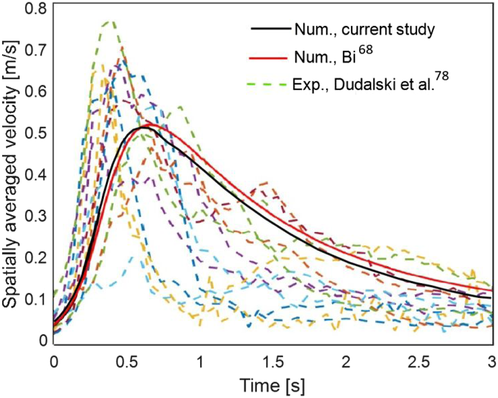
In this study, different simulations were performed to investigate the effects of relative humidity and ambient temperature on droplet behaviour. Although the simulations are not perfectly matched with the experiment due to experimental limitations and different time scales investigated, they are representing a standard human cough. Indeed, measuring the velocity profile at the mouth is challenging and requires specific instruments such as PIV, and it was not measured in our experiments. Thus, as mentioned, a velocity profile from the work of Gupta et al., ⁴⁹ which demonstrates a real cough with an average velocity (i.e. 8.808 m/s) close to that of our experimental data was used. We believe that a great qualitative understanding of what happens to the droplets upon cough occurrence can be gained by the comparison between the experiments and the simulations. Due to computational limitations, the simulations were run for only 6.21 s. As can be seen in the results, even this short period is able to provide insights into the details of droplet behaviour comprehensively.

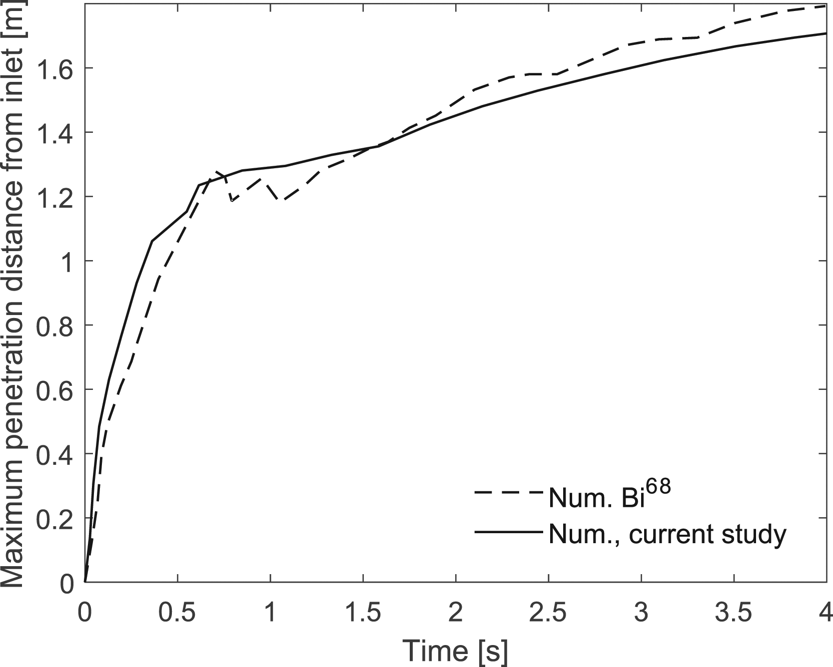
To show the mesh quality and validate the numerical results, the results obtained from the present study were compared with the experimental data measured by Dudalski et al. ⁷⁸ using a PIV system and the numerical study of Bi. ⁶⁸ The measurements were performed inside a rectangular field of view (0.09 × 0.48 m²) located 1 m downstream of the mouth. In total, 7 influenza-infected participants were enlisted for the experimental investigations and 13 sets of cough data were chosen. As can be seen in Figure 7, the experimental data varies significantly, proving that the cough flow strongly depends on human physiology. To present this figure, the results of the current study as well as Bi’s numerical data were obtained from the mentioned field of view. As shown, there is a good agreement between the numerical results obtained in the present study and experimental data as well as Bi’s numerical results. For the 13 coughs, the maximum value of averaged velocity changes between 0.2 and 0.77 m/s. While for the numerical studies, it is around 0.52 m/s. In addition, the maximum penetration distance of droplets from the inlet was calculated in the current study, and was compared with the numerical results of Bi. ⁶⁸ As shown in Figure 8, the maximum penetration distance increases with time and there is a good agreement between the numerical results. To plot Figure 8, RH and air temperature were fixed at 50% and 21°C, respectively.

Figure 7.

Comparison between the numerical results obtained from the current study and experimental and numerical studies in the literature.^68,78

Figure 8.

Comparison of the maximum penetration distance of droplets obtained in the current study and Bi’s work. ⁶⁸

Results and discussion

Images of the cough progression are shown in Figure 9. The axis of symmetry was illuminated using a 5-W continuous-wave diode-pumped solid-state laser. The laser beam was converted into a diverging light sheet using a pair of cylindrical lenses. The images were taken using a 16-bit scientific CMOS camera and a wide-angle lens of 30 mm focal length. The camera timing was synchronized with the cough initiation using the internal clock of the digital delay generator. From the images, the cough flow was highly turbulent and took about 100 ms for the cough to develop. The aerosol was diluted at an increasing rate with an increasing distance from the manikin, evidenced by a reduction in scattering light intensity. At 400 ms, the cough was a very fast jet with a reduced dispersion angle. The turbulent eddy structures in the wake of a cough were visible in the post-cough image.

Figure 9.

Images of the cough at five different times after the cough initiation. The field was illuminated using a 5-W continuous-wave laser beam converted into a laser sheet by cylindrical laser optics. The exposure time was kept constant at 5 ms.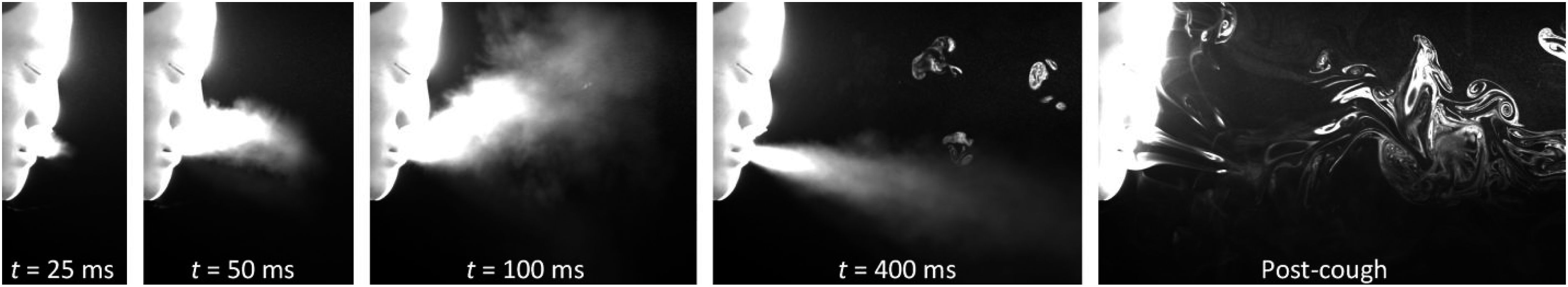

The number of aerosol nuclei per unit volume for all 6 bins plotted as a function of time starting from the cough initiation is presented in Figure 10 for a sampling location of 0.5 m away from the manikin’s mouth (location 2). The results show that the maximum aerosol concentration for nuclei sizes of 0.5+ µm was reached within a few minutes after the cough and decayed to almost background levels within an hour. The droplet nuclei counts for the size bins of 0.3, 0.5 and 1.0 µm were about the same order of magnitude. The nuclei counts for the size bins of 3.0, 5.0 and 10.0+ µm were 2, 4 and 5 orders of magnitude less than that of smaller nuclei, respectively. The droplet nuclei larger than 10 µm returned to background levels 10 min after the cough. This was expected because of the higher sedimentation as well as evaporation rates of larger droplets. The droplet nuclei count within 5- to 10-µm size bins showed an initial spike a few minutes after the cough and a second peak at about 10 min. The former spike is believed to be due to the bulk transport of the aerosol plume by the cough momentum, and the latter was due to diffusion from the stagnant cough plume. One interesting observation was that the droplet nuclei within 0.3–0.5 µm showed a gradual increase up to 40 min and a decay afterwards. We believe that this is due to the droplet nuclei from larger size bins feeding this bin as larger droplets lose mass due to evaporation. There was still a significant quantity of droplet nuclei of 0.3–1.0 µm present within the space 70 min after the cough.

Figure 10.

Droplet nuclei count measurements for six size bins of 0.3, 0.5, 1.0, 3.0, 5.0 and 10+ µm from a sampling location of 50 cm in front of the manikin’s mouth (location 2). The shaded region represents the standard deviation of the average over five measurements.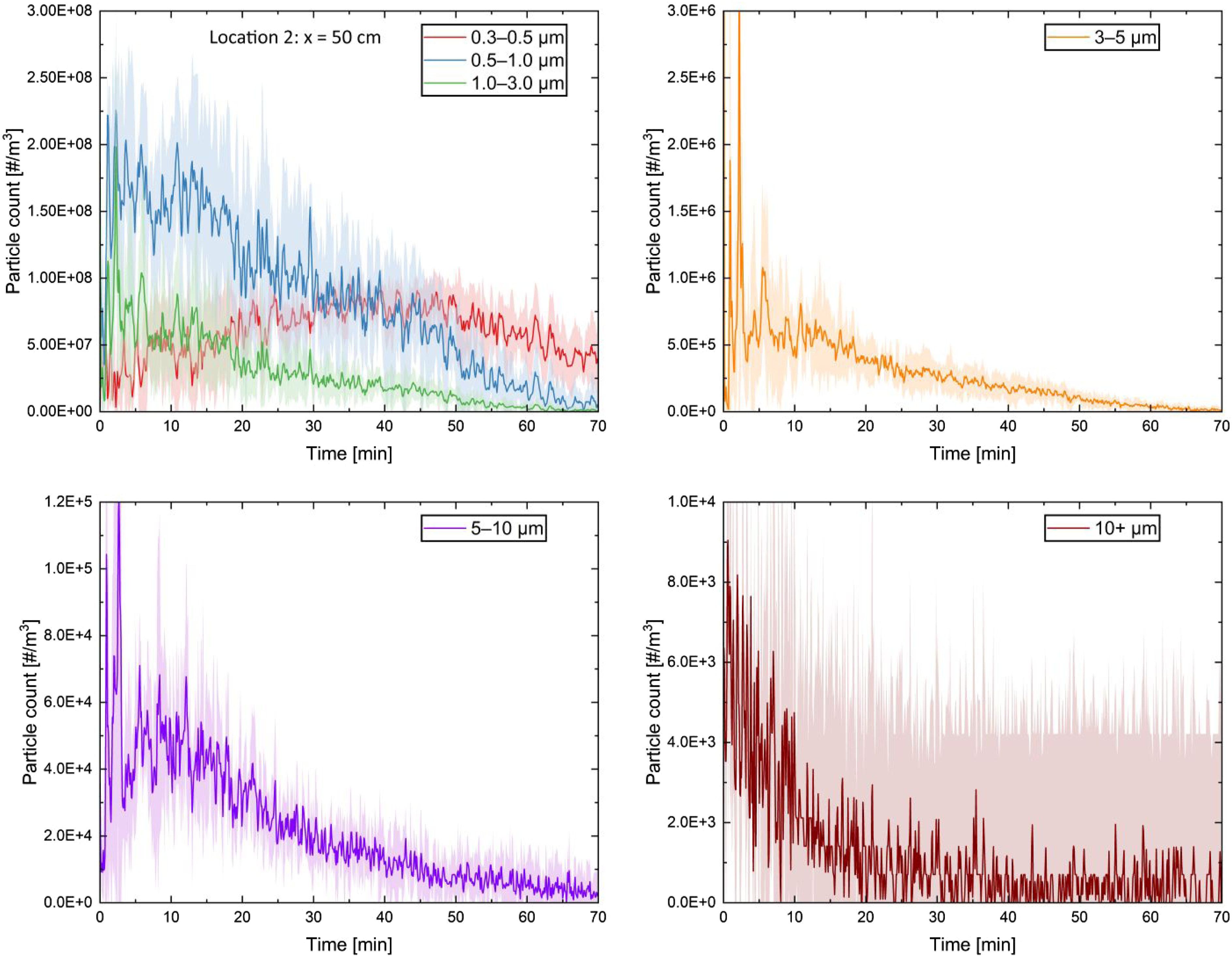

The particle trajectories (showing the history of droplet locations within the domain) from the numerical simulations over 6.21 s are shown in Figure 11 which helped to obtain a sense of how droplets travel. A general observation of the shape exhibited by the tracks is that while most of the expelled particles travel horizontally for some distance before falling to the ground, there is a smaller portion of particles that begin to travel upwards above the horizontal at the inlet, showing that some particles are remaining suspended in air over time instead of all falling to the ground after expulsion. This observation demonstrates the reality that a cough travelling through the air can induce airborne virus transmission. The contour plot in the image to the left displays the range of particle diameters among the tracks, which shows that particles in the larger diameter ranges are travelling further horizontally from the inlet and are meeting their fates on the ground. However, most of the particles around the 1.2-µm diameter range travel upwards and do not fall to the ground. Furthermore, the contour plot on the right displays the particle velocities over their lifetime, where many of the particles that are falling to the ground maintain a higher velocity over their lifespan, while the particles that travel upwards become very slow and stagnant near the end. From these two plots created from the numerical simulations, very small particles are clearly shown to remain suspended in the air after a cough, as they tend to travel upwards and slow down significantly.

Figure 11.

Particle trajectories over 6.21 s from numerical simulations showing particle diameter contours (left) and particle velocity contours (right).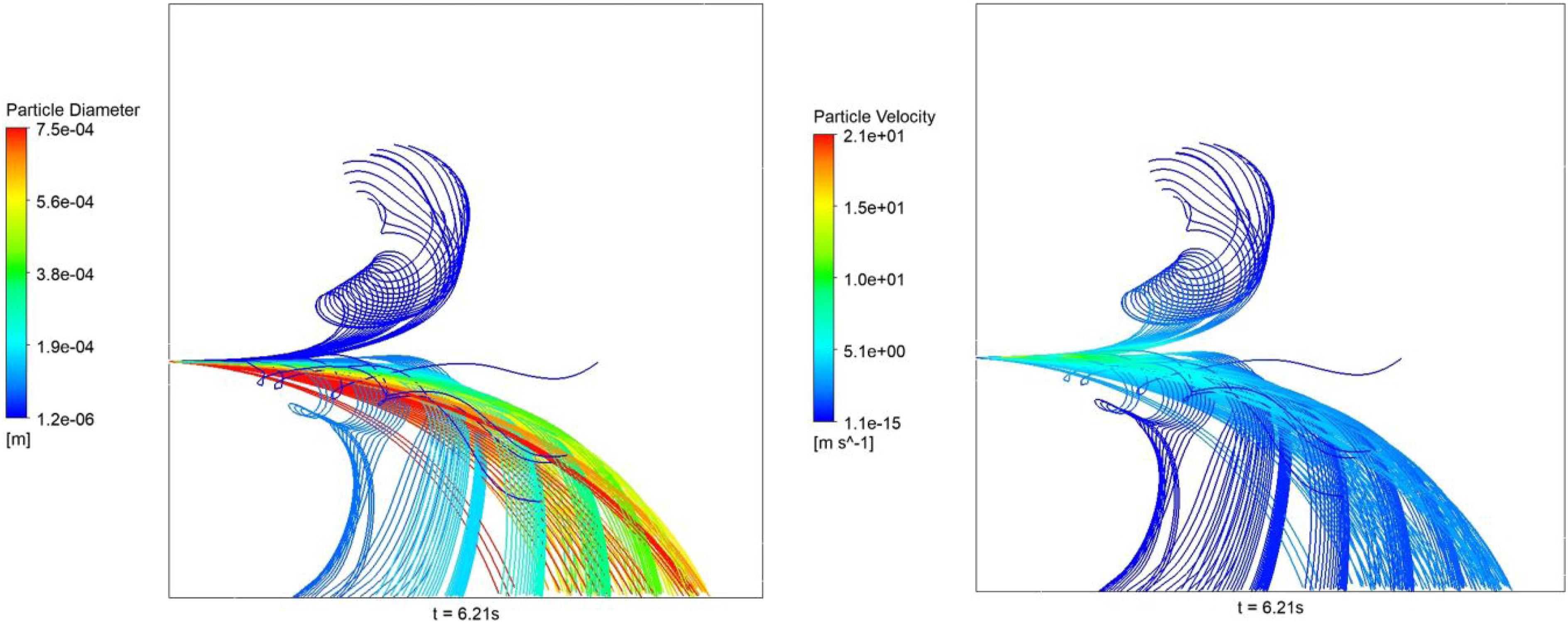

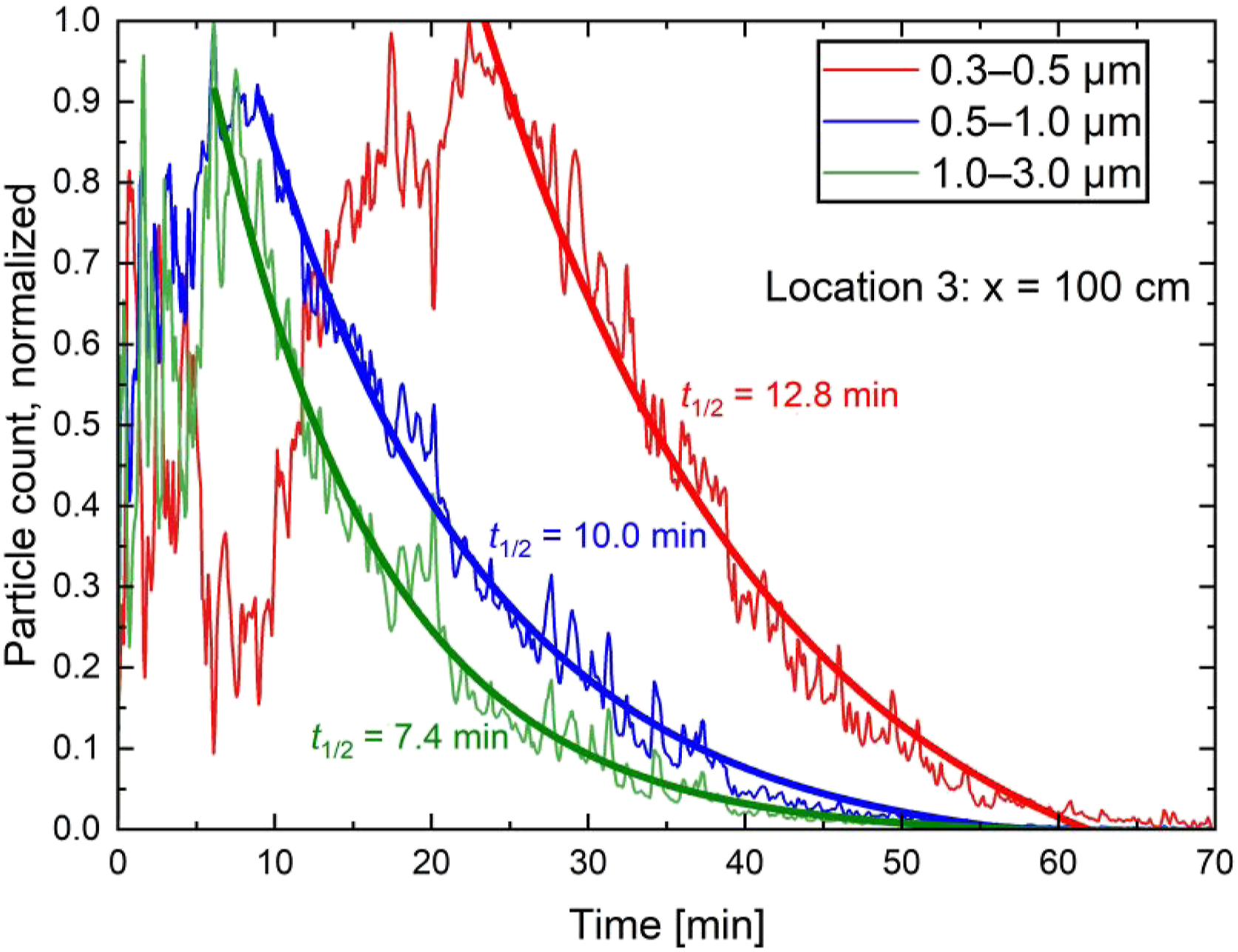
In the experiments, decay of the droplet nuclei concentration was dependent on the measurement location. The decay was found to obey an exponential decay function defined by equation (7)

$y=y_0+A_1{e}^{-\left(x-x_0\right)/t_1}$

(7)

where $y$ is the droplet nuclei count, $x$ is the time, $x_0$ and $y_0$ are x- and y-axes offsets, $A_1$ is the amplitude and $t_1$ is the time constant. The decay half-life, $t_{1/2}$ , can be calculated from the time constant as $t_{1/2}=t_1\times \text{ln}\left(2\right)$ . Figure 12 shows the decay rates and corresponding half-lives for 0.3-, 0.5- and 1.0-µm size bins for a sampling location of 1 m in front of the manikin (location 3). The nuclei counts are normalized in Figure 12. Although the peak was reached at different times for different size bins, all droplet nuclei decayed to background levels at 60 min proceeding the cough. The smallest aerosol nuclei, that is, 0.3–0.5 μm, decayed the slowest with a half-life of 12.8 min. The droplets corresponding to 0.5- and 1.0-μm size bins decayed faster with half-lives of 10.0 and 7.4 min, respectively. This is expected as larger aerosol is known to evaporate at a faster rate and has a higher sedimentation rate. To no surprise, the half-lives of droplets within the 10+ μm size bin (not shown) were even shorter, 4.5 min.

Figure 12.

Normalized droplet nuclei count for three size bins of 0.3, 0.5 and 1.0 µm from a sampling location of 100 cm in front of the manikin’s mouth (location 3). An exponential decay fitting was performed based on equation (7), represented as thicker lines originating from maximum droplet nuclei counts.

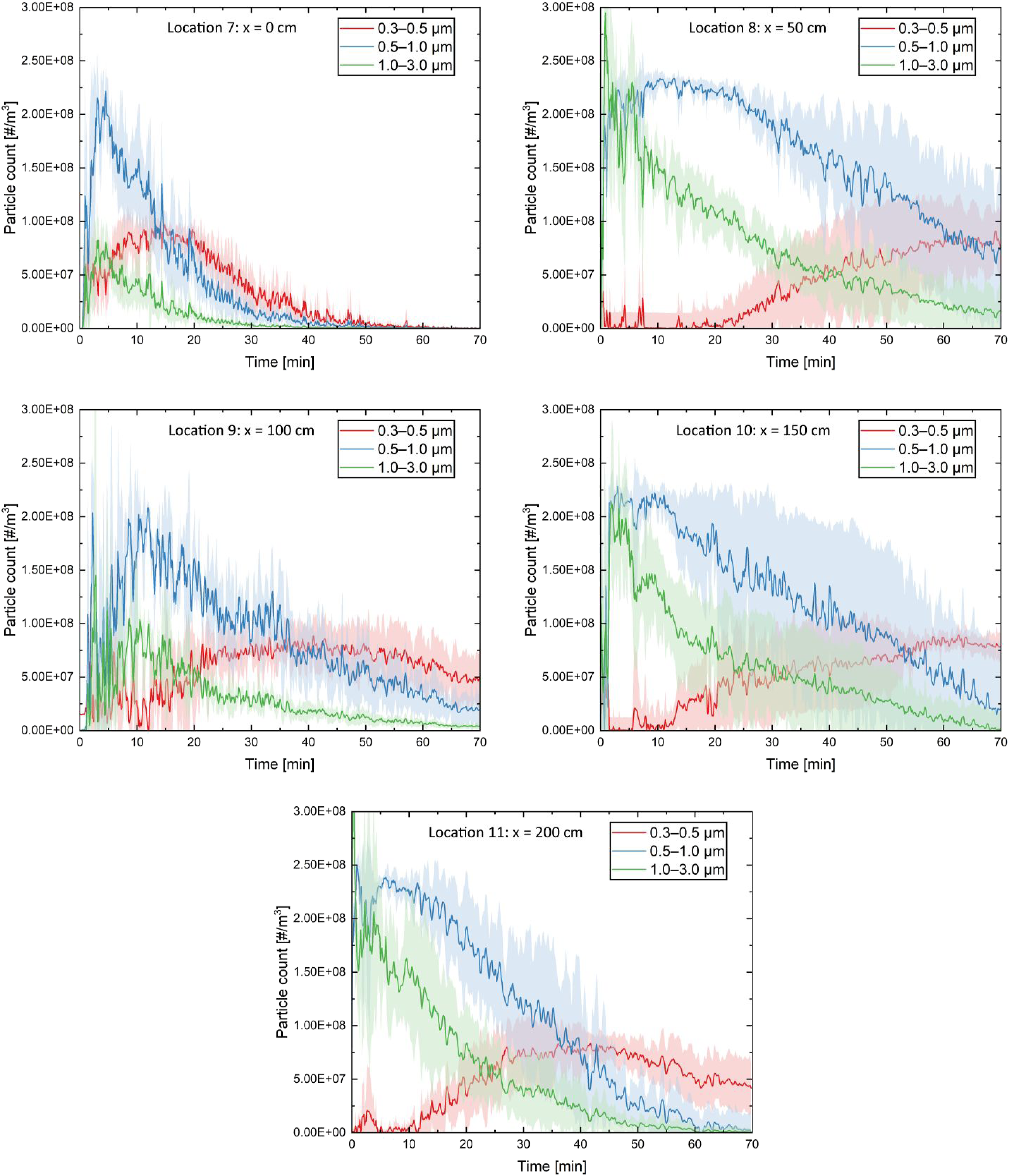
Droplet nuclei count measurements for size bins of 0.3, 0.5 and 1.0 µm for six locations on the cough plane and five locations 0.8 m offset to the cough plane are presented in Figure 13 and Figure 14, respectively. The orders of nuclei counts were similar for all locations at 10⁸ particles per m³ of air. However, the decay rates showed some variability. Data collection for each location has taken about 8 h and was performed in a single day.

Figure 13.

Droplet nuclei count measurements for three size bins of 0.3, 0.5 and 1.0 µm from six sampling locations within the cough plane (locations 1–6). The shaded region represents the standard deviation of the average over five measurements.

Figure 14.

Droplet nuclei count measurements for three size bins of 0.3, 0.5 and 1.0 µm from five sampling locations on a parallel plane 80 cm offset to the cough plane (locations 7–11). The shaded region represents the standard deviation of the average over five measurements.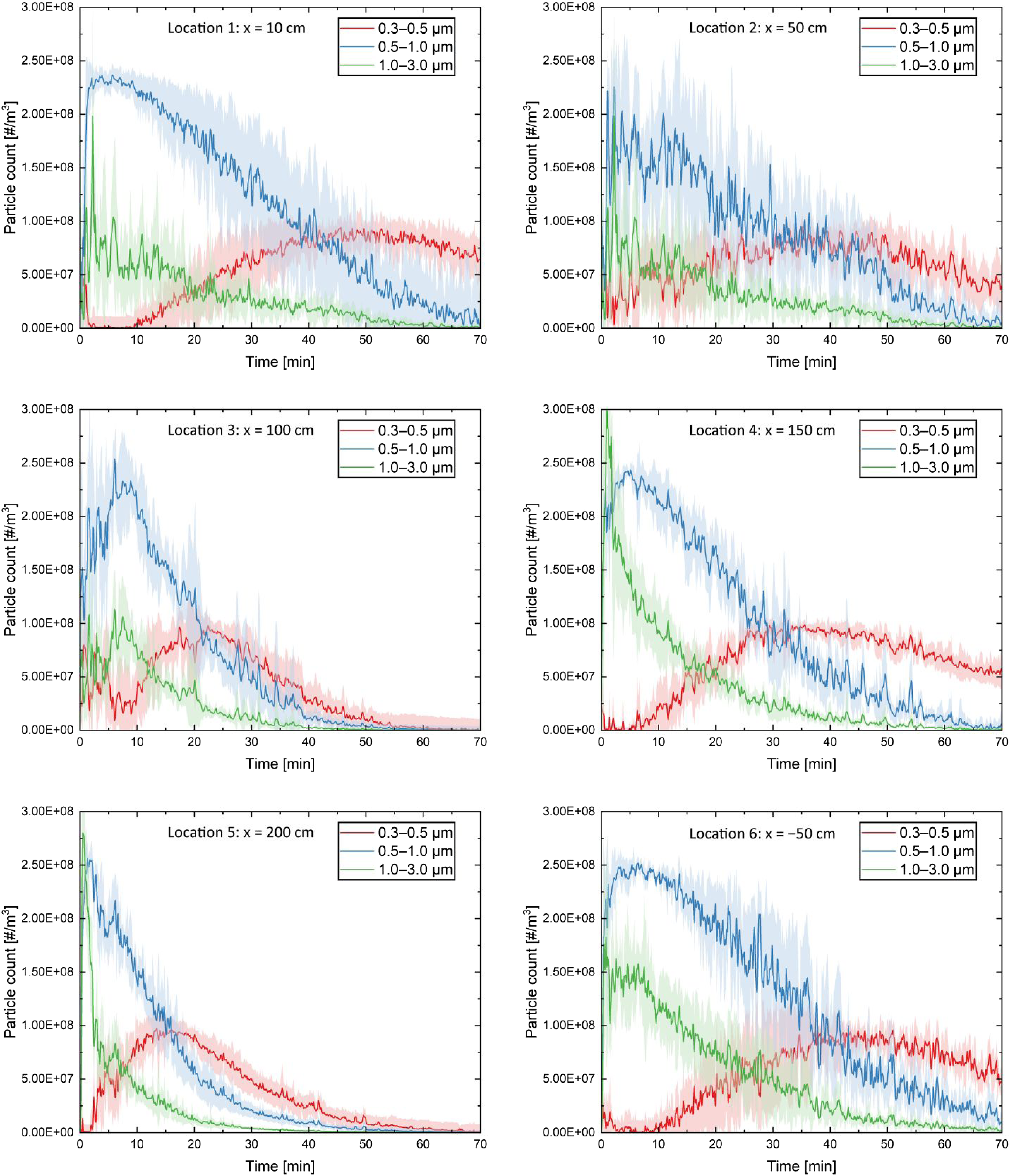

The variability in the viral decay rates might be due to effects of air temperature and RH. Dabisch et al. ³⁰ showed that the increase in temperature and RH would result in a decrease in the virus stability and airborne decay. They also found that the temperature has a much greater influence on viral decay than humidity. As shown in Table 2, the temperature was slightly varied in the present study which could have affected the results; however, its range is representative of conditions expected indoors. The variation in the humidity was in a wider range but the effect has already been studied by several researchers.^29,30 Therefore, acutely controlling the humidity in the experiments, while interesting, was beyond the scope of the present study; however, in the modelling component, the humidity was controlled and the sensitivity to humidity was evaluated.

In addition to the ambient conditions, the cough dispersion was highly turbulent as can be observed in Figure 9. We believe that this variability is a result of the chaotic nature of turbulence and different climate conditions, which are known to affect diffusion, evaporation and sedimentation rates. The numerical simulations that were performed to display the differences in cough dispersion were based on the climate conditions, including the ambient temperature and relative humidity. The results of these simulations, which are discussed below, show that the differences in such climate conditions indeed could affect the trajectories, evaporation rate and the size of droplets. These effects were caused by varying climate conditions and can help explain the variance in the cough dispersion that was observed in the experimental data. In the combined 11 locations presented in Figures 13 and 14, only 3 displayed aerosol counts return to background levels in 70 mins proceeding the cough; the remainder had significant aerosol remaining, especially in the 0.3- to 0.5-μm size bin. There was no significant difference between measurements from the cough symmetry plane and a parallel plane 0.8 m offset to the symmetry plane. One sampling location of significant interest was location 6 which was on the cough symmetry plane 0.5 m behind the manikin. Aerosol droplets could only be transported to this location by circulation and diffusion. This is a direct proof that given enough time, aerosol would disperse more or less evenly following the cough jet into a still environment.

To show the effect of humidity on particle behaviour, the ambient conditions used in the numerical simulations for temperature were held constant at 25°C, and a cough was simulated for each of three tested relative humidities, being 30%, 50% and 80% water vapour saturation in the air. The results of these simulations are shown in Figure 15 and Figure 16, which show the total number of particles suspended within the domain (i.e. particle count) over time as well as the average diameter of suspended particles over time, respectively. The data were collected in a region between the inlet and a plane located 1 m from the inlet. As shown in Figure 15, all the droplets were injected into the domain by 0.13 s, when the particle count reached its peak value. Subsequently, the particle counts in all cases declined with time due to precipitation of the large droplets, coalescence and evaporation. As shown by the figure, the increasing RH would cause the number of suspended particles to enhance. This shows that the increasing RH would slow down the evaporation, coalescence and precipitation of particles. In addition, after roughly 0.5 s, the rate of change of particle counts with time would decrease, which is mainly owing to the dispersion of particles and reduction in particle coalescence and precipitation.

Figure 15.

Particle counts versus time with ambient temperature constant at 25°C and with the varying relative humidity at 30%, 50% and 80%.

Figure 16.

Average particle diameter versus time with a constant ambient temperature at 25°C and the varying relative humidity at 30%, 50% and 80%.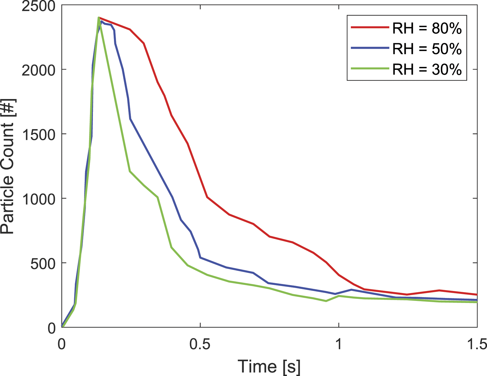

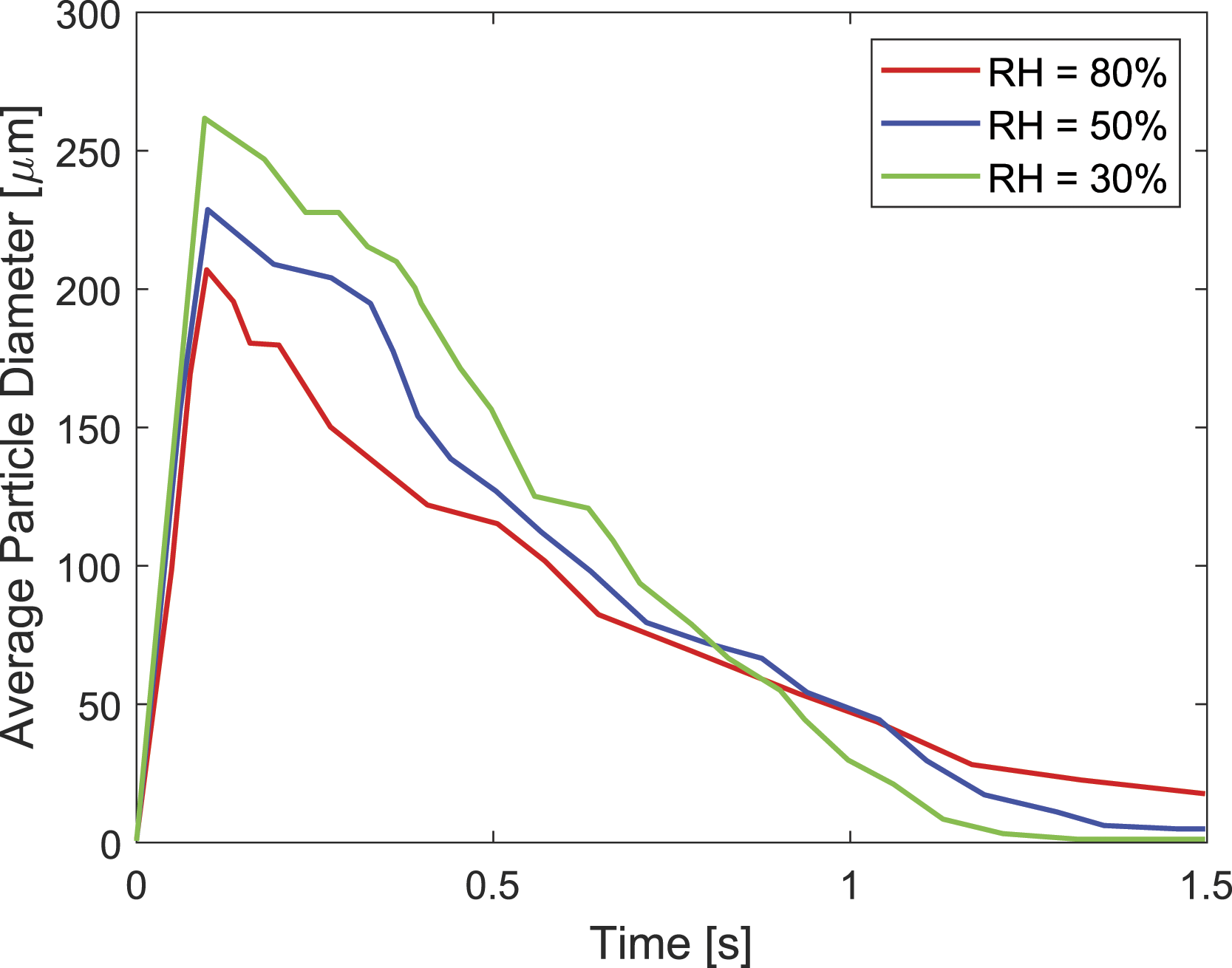
In Figure 16, the average diameter was increased rapidly in all the cases until 0.13 s due to the particle injection. Subsequently, a sharp decline of the particles was observed until roughly after 1 s, and then the average diameter was reduced gradually with time. After particle injection, when the time was between 0.13 and 0.5 s, the coalescence phenomenon became dominant and affected the average diameter significantly. As shown in Figure 15 and Figure 16, the case with RH = 30% produced the lowest particle counts and the largest average diameter, which indicates that the decreasing RH can enhance the coalescence rate significantly (in other words, the diameters of particles would increase and the number of particles would decrease due to the collision of particles). Afterwards, due to particle dispersion, the importance of particle collision would decrease, and precipitation and evaporation would become dominant. In other words, the particle counts and average diameter would decrease due to the precipitation and evaporation of the particles. After approximately 1 s, a different trend emerges and higher RH results in a greater average diameter as evaporation dominates, reducing the particle diameter. Evaporation is a strong function of RH, and the evaporation rate would decrease with an increase in RH. As a result, the case with RH = 80% produced the largest average particle diameter and particle counts.

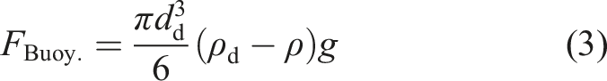
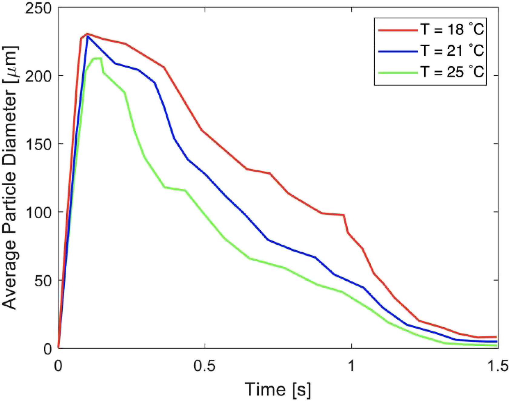
The effects of temperature on droplet behaviour were examined through the plots as shown in Figure 17 and Figure 18. In both figures, the ambient relative humidity was held constant at 50% while the ambient temperature was varied across simulations at 18°C, 21°C and 25°C. Similar to the previous figures, Figures 17 and 18 show the particle counts and the average particle diameter versus time, respectively, both measured in a region between the inlet and a plane located 1 m from the inlet. In Figures 17 and 18, over time, with the rise in temperature, both particle counts and average particle diameter were shown to have decreased. Two reasons for this behaviour were noted: (1) increasing air temperature would cause the evaporation of particles to become faster. Consequently, the average particle diameter would be reduced, and since many small particles would be fully evaporated, the number of suspended particles would decrease as well. (2) The suspension of the droplets is mainly due to buoyancy that was induced by the temperature difference. In fact, the buoyancy force would depend directly on the air density and the particle diameter (see equation (3)). By increasing the air temperature, both the air density and the particle diameter (due to higher evaporation rate) would decrease. Therefore, the buoyancy force was shown to decrease, which increased the rate of precipitation. A similar discussion was recently presented by Zhang et al. ⁷⁹ In Figures 15‒18, the trends did not change after 1.5 s, and the curves gradually approached zero.

Figure 17.

Particle counts versus time with the ambient relative humidity set at 50% and with a varying temperature at 18, 21 and 25°C.

Figure 18.

Average particle diameter versus time with the ambient relative humidity set at 50% and with a varying temperature at 18, 21 and 25°C.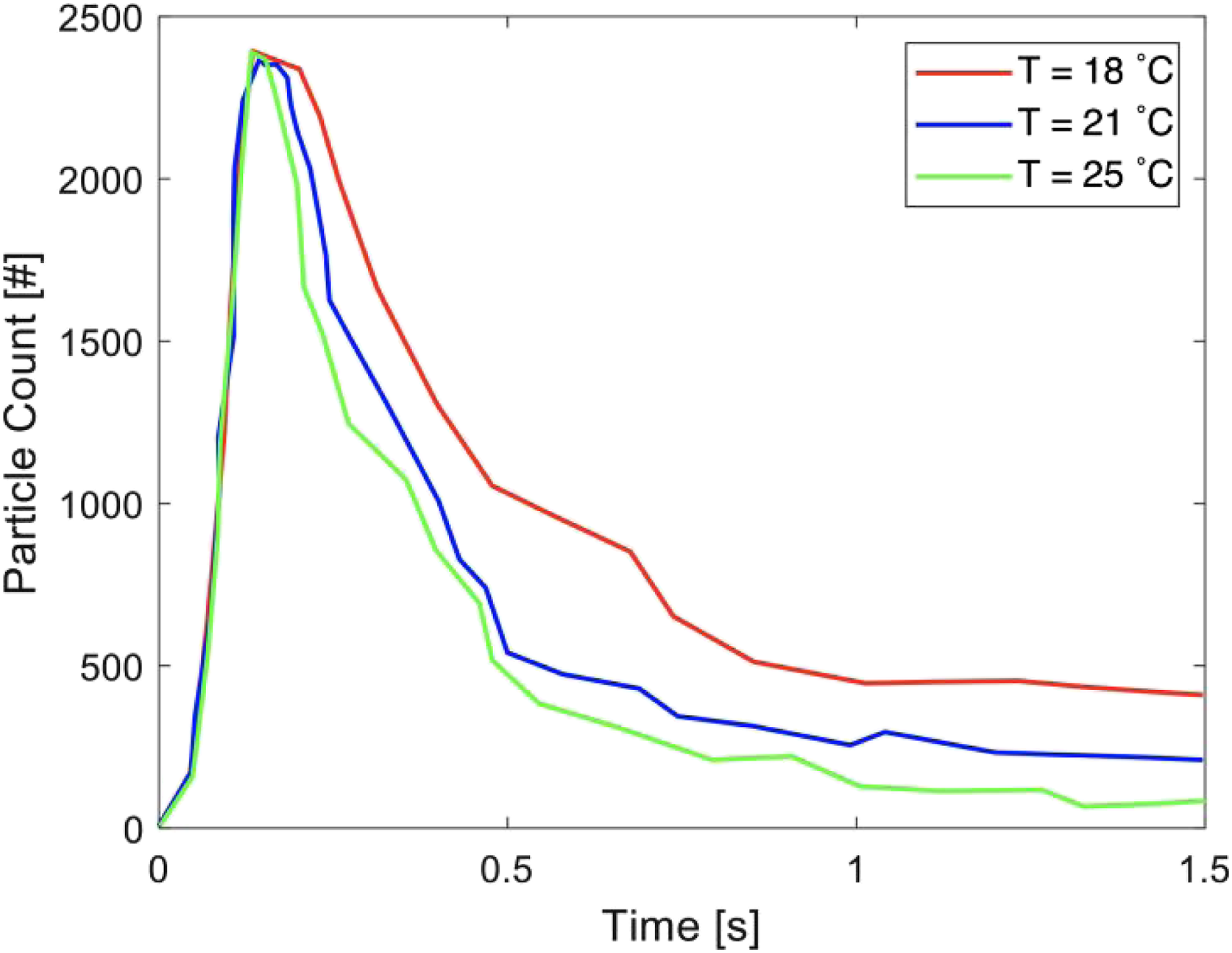

By comparing the results of the numerical simulations, both ambient temperature and ambient relative humidity were shown to have a great effect on droplet activity (similar results have been reported by Bi, ⁶⁸ Redrow et al., ⁸⁰ Yan et al. ⁷² and Zhang et al. ⁷⁹ ). Not only do temperature and humidity affect the number of droplets remaining in the domain, but also the size of these droplets. As particle sizes are decreasing with humidity and increasing temperature, their chances of evaporation are greatly increased, which can lead to higher rates of airborne virus transmission. ⁶⁸ With this information, we recommend the controlling of both the temperature and humidity in indoor spaces should be treated with great importance.

To better understand aerosol lifetime, data corresponding to all sampling locations were averaged. The black line in Figure 19(a) displays the total droplet nuclei counts that were summed over all nuclei counts from all size bins, which were averaged for all sampling locations (locations 1–11) and normalized. The shaded region represents the standard deviation of the average over 11 measurements from all sampling locations. The peak aggregate droplet nuclei count was reached after 2.2 min proceeding the cough and decayed exponentially afterwards. The coefficient of determination for fitting the exponential decay given by equation (7) was very high at 0.996. The droplet half-life was calculated as 43 min. In a still environment, aerosol of 0.3- to 10-µm size persists for a very long lifetime, which has significant implications for airborne disease transmission. A significant number of aerosols, that is,. 20% of the maximum nuclei count, would still be present at 70 min proceeding the cough. The blue line in Figure 19(a) represents the total aerosol exposure, calculated by integrating the absolute nuclei count. With a half-time of 43 min, a significant exposure is possible even hours following the aerosol release. Figure 19(b) displays the same plot as Figure 19(a) but zoomed in for the first 3 min following the cough. As shown in Figure 19(b), the maximum droplet nuclei count was achieved at 2.2 min following the cough.

Figure 19.

Aggregate sampling measurement results: (a) Total droplet nuclei count measurements from all size bins displaying, these were averaged for all sampling locations (locations 1–11) and normalized. The blue line represents the total exposure as a function of time; (b) same as (a) plotted versus the initial 3 min proceeding cough initiation; and (c) total droplet nuclei volume calculated from nuclei count measurements and average nuclei diameters for all size bins, averaged for all sampling locations (locations 1–11) and normalized. The shaded regions in (a)‒(c) represent the standard deviation of the average over 11 measurements at different sampling locations.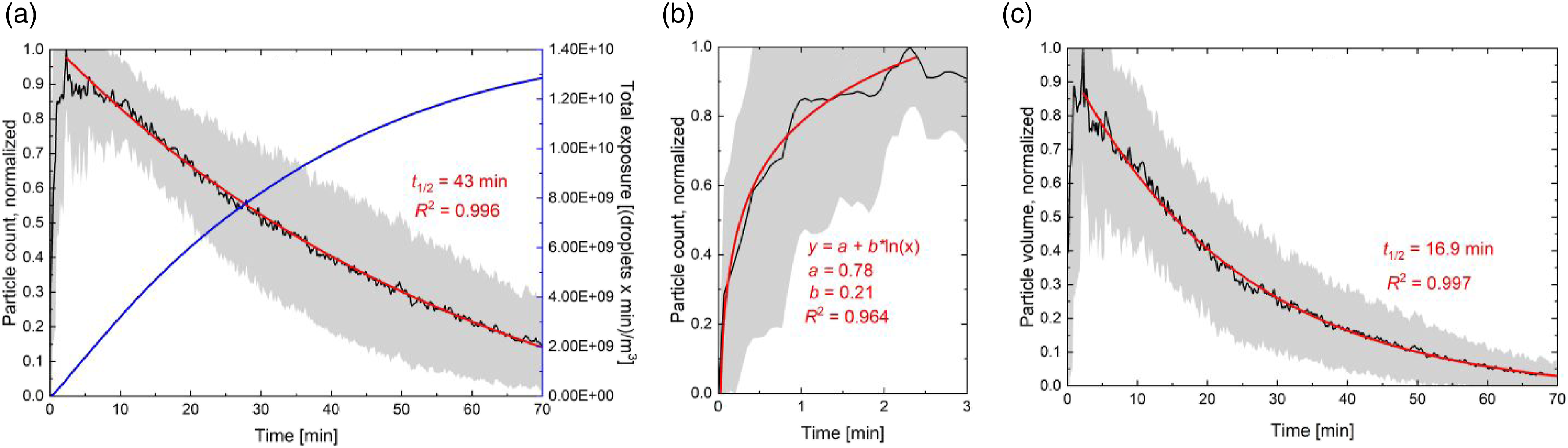

The droplet nuclei count growth due to the initial cough dispersion can be represented with a logarithmic regression function defined by $y=a+b\text{ln}\left(x\right)$ , where $y$ is the droplet nuclei count and $x$ is the time. The constants $a$ and $b$ were calculated as 0.78 and 0.21, respectively. Lastly, Figure 19(c) presents the combined droplet nuclei volume of all aerosols averaged for all sampling locations (locations 1–11) and normalized. The shaded region represents the standard deviation of the average over 11 measurements from all sampling locations. For droplet counts to volume conversion, average droplet diameters of 0.4, 0.75, 2.0, 4.0, 7.5 and 10 µm were chosen for particle size bins of 0.3, 0.5, 1.0, 3.0, 5.0 and 10.0+ µm, respectively. The aerosol volume per unit air rather than the nuclei counts would be a better representation of the airborne virus presence as bigger droplets were assumed to contain more viruses. Once again, the decay of the aerosol volume with time can be very accurately represented using the exponential decay function defined by equation (7). The decay half-life was found to be about 17 min, much smaller than the 43 min calculated for droplet nuclei counts. This reduction was expected because there is more volume contained in bigger droplets which would evaporate and drop as sediment at a higher rate.

To understand the dispersion and lifetime of droplets under HVAC condition, we measured the total aerosol volume with and without simulated HVAC, presented in Figure 20. The HVAC port was connected to the ceiling of the enclosure (see Figure 3). The port has an area of 500 cm², and air was removed from the enclosure at a rate of 8 m³/min. The measurements were taken from 1 m in front of the manikin (location 3) and performed on the same day to prevent variations due to climate conditions. The results are very striking; the half-life of droplet volume was reduced from 28.9 min to 0.7 min with the addition of air ventilation. During the pandemic post-opening and for other airborne diseases, infrastructural changes such as the redesign of HVAC systems incorporating considerations for aerosol dispersion as well as restoration of existing buildings with more effective air circulation would be of great importance. The main goal of the ventilation experiment in the present study was to demonstrate the drastic effect the HVAC could provide in terms of reducing the risk of pathogen transmission. Ventilation systems should be properly designed and operated for each environment. This is not within the scope of the current study and the interested readers are referred to the works of Li et al.^81–84 and Lipinski et al. ⁸⁵ for more information about ventilation strategies.

Figure 20.

Total droplet nuclei volume calculated from nuclei counts of all size bins and average nuclei diameters corresponding to a sampling location of 100 cm in front of the manikin (location 3). The blue line corresponds to stagnant environmental conditions, and the red line corresponds to simulated HVAC.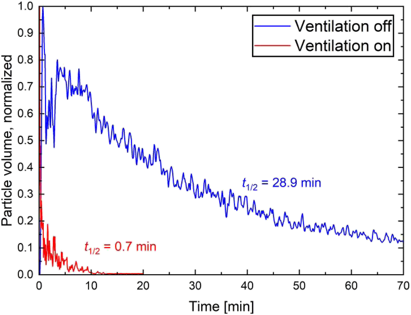

Summary and conclusions

In the present study, the spatial and temporal dispersion of aerosol droplets at different sizes have been experimentally and numerically investigated. A novel cough generator was designed and built that can generate repeatable respiratory ejecta with user-defined parameters. Aerosol dispersions at various size bins were measured at 11 different locations over 1 h. Five locations are along the direction of the cough, one location is 0.5 m behind the mouth in the opposite direction of the cough and the rest are in a plane located 0.8 m to the side of the mouth. The droplet nuclei concentration was found to follow an exponential decay function with a characteristic half-life that increases with the decreasing droplet size. In addition, the measurements from different locations (including the one behind the mouth) show similar trends, demonstrating that aerosols can disperse almost uniformly into a still environment over a very long duration due to diffusion.

By averaging the data corresponding to all sampling locations, the rising droplet nuclei counts were found to reach a peak value and then declined exponentially. Furthermore, aerosols of 0.3- to 10-µm size would remain in a still environment for a very long time, which can enhance airborne disease transmission. Indeed, around 20% of the maximum nuclei count exists after 70 min after the cough.

Numerical simulations were performed using the Eulerian–Lagrangian approach to show the influence of ambient conditions on the droplet trajectory, surviving droplet diameter and concentration, to explain the physical phenomena observed in experiments. Some small droplets were found to remain suspended in the air over time instead of falling to the ground. In addition, the ambient condition can have a considerable influence on the droplet concentration and in-air behaviour.

Lastly, the air ventilation can reduce the total aerosol volume and the droplet lifetime significantly, demonstrating the importance of HVAC systems in buildings and indoor environments.