The Facility Infection Risk Estimator™: A web application tool for comparing indoor risk mitigation strategies by estimating airborne transmission risk

Abstract

The COVID-19 pandemic created needs for (a) estimating the existing airborne risk of infection from SARS-CoV-2 in existing facilities and new designs and (b) estimating and comparing the impacts of engineering and behavioural strategies for contextually reducing that risk. This paper presents the development of a web application to meet these needs, the Facility Infection Risk Estimator™, and its underlying Wells–Riley based model. The model specifically estimates (a) the removal efficiencies of various settling, ventilation, filtration and virus inactivation strategies and (b) the associated probability of infection, given the room physical parameters and number of individuals infected present with either influenza or SARS-CoV-2. A review of the underlying calculations and associated literature is provided, along with the model's validation against two documented spreading events. The error between modelled and actual number of additional people infected, normalized by the number of uninfected people present, ranged from roughly –18.4% to +9.7%. The more certain one can be regarding the input parameters (such as for new designs or existing buildings with adequate field verification), the smaller these normalized errors will be, likely less than ±15%, making it useful for comparing the impacts of different risk mitigation strategies focused on airborne transmission.

Introduction

At the beginning of the pandemic in early 2020, there was an expressed need from various building owners, facility managers, occupants and architecture, engineering, and construction (AEC) industry consultants to help evaluate the relative contribution of different interior COVID-19 risk mitigation strategies. There was a lack of easily accessible tools and other resources for comparing and ranking different engineering and behavioural strategies (e.g. increased ventilation, filtration, mask wearing, de-densifying, germicidal ultraviolet technologies, etc.) for a given context based on both (a) removal efficiency and (b) the probability of infection. The model presented in this paper and its web-based application ¹ were developed specifically to contextually compare and rank available influenza and SARS-CoV-2 mitigation strategies for making any built environment safer with respect to far-field virus-containing aerosols. Other modes of transmission exist with varying degrees of relevance for different pathogens, such as fomite or direct physical contact. Additional risk mitigation strategies associated with these other modes of transmission, such as surface cleaning, are not included in this model. However, the consensus among many scientists at this point is that the dominant route of transmission of SARS-CoV-2 is airborne. ² There is increasing evidence that this also applies to influenza and other respiratory viruses,^3–5 further indicating a need for tools capable of evaluating the risk mitigation potential relative to airborne transmission.

Airborne in this case refers to the transmission of viral particles or other pathogens from an infected individual through the air to an uninfected individual who inhales a quantity of particles sufficient to result in infection. Aerosols expelled from the infected individual act as the transport ‘vehicles’ for the pathogens and depending on their size and environmental conditions, may float in the air for hours or even days. Aerosol science indicates that drops of respiratory fluid approximately 100 µm and less in diameter may float and evaporate faster than they fall to the ground (though it is not a hard boundary), ⁶ and therefore for the purposes of this paper are termed aerosols (sometimes labelled droplet nuclei). Also for the purposes of this paper, respiratory fluid larger than 100 µm in diameter are labelled droplets and will generally fall to the ground faster than they evaporate.

Far-field aerosols refer to aerosols beyond roughly six feet from an infected person, and their concentration level is generally closer to the whole room average aerosol concentration level than for near-field aerosols. ⁷ Near-field aerosols refer to aerosols within roughly six feet of an infected person and occur at higher concentration levels than far-field aerosols (though as they dissipate throughout the room, they eventually become far-field aerosols). Far-field aerosols are impacted more than near-field aerosols by most of the mitigation strategies focused on by this model which also have very little to no impact on droplets (with settling and masks being the notable exception).

The objectives of this study are to (1) provide a detailed review of the mathematical models and published data that describe droplet/aerosol generation and quantum generation of an infected occupant, removal and inactivation mechanisms and the corresponding infection risk reduction of different strategies; (2) develop a comprehensive model that can compare and rank those strategies; (3) validate the model against two documented super-spreading events of SARS-CoV-2 and (4) assess the model’s general effectiveness. The authors also discuss the model’s limitations as well as its assumptions and justifications.

Modelling aerosol transmission and literature review

The probability of infection calculations used by the model of the Facility Infection Risk Estimator™ ¹ are based on a modified version of the Wells–Riley model of infection.^8,9 The starting point ⁹ for this model includes removal terms for ventilation, building system filtration and settling. Removal terms for portable air cleaners, masks, inactivation from relative humidity (RH) and inactivation from upper room UVGI (ultraviolet germicidal irradiation) were subsequently added. The modified formula is equation (1)

$$P=\left[1-\exp (\frac{-\left(q\text{\hspace{0.17em}×\hspace{0.17em}}I\text{\hspace{0.17em}×\hspace{0.17em}}p\text{\hspace{0.17em}×\hspace{0.17em}}s\text{\hspace{0.17em}×\hspace{0.17em}}t\right) }{\mathrm{V}\text{×}\left({\mathrm{k}}_{\mathrm{settling}}+{\mathrm{\lambda }}_{\mathrm{ventilation}}+{\mathrm{k}}_{\mathrm{filtration}}+{\mathrm{k}}_{\mathrm{RHinactivation}}+{\mathrm{k}}_{\mathrm{UVGinactivation}}+{\mathrm{k}}_{\mathrm{aircleaner}}+{\mathrm{k}}_{\mathrm{mask}}\right)})\right]\text{×}{\mathrm{v}}_{\mathrm{adjusted}}$$

(1)

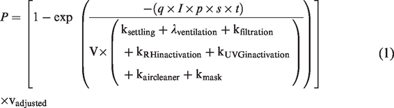
P = probability of infection

q = quantum of infection (quanta generation rate), discussed further below

I = number of infected individuals, discussed further below

p = pulmonary ventilation rate, discussed further below

s = modified p scaling factor for masks, discussed further below

t = time of exposure, discussed further below

V = volume of the room/space

k_settling = settling removal factor, discussed further below

λ_ventilation = ventilation removal factor, discussed further below

k_filtration = building system filtration removal factor, discussed further below

k_{RHinactivationIVA} or k_{RHinactivationSC2} = RH inactivation removal factor, discussed further below

k_{UVGIinactivationIVA} or k_{UVGIinactivationSC2} = upper room UVGI inactivation removal factor, discussed further below

λ_aircleaner = portable air cleaner removal factor, discussed further below

k_mask = mask removal factor, discussed further below

v_adjusted = adjusted vaccination factor, discussed further below.

Quantum of infection

The Wells–Riley model is

… based on a concept of ‘quantum of infection, whereby the rate of generation of infectious airborne particles (or quanta - q) can be used to model the likelihood of an individual in a steady-state well-mixed indoor environment being exposed to the infectious particles and subsequently succumbing to infection. ⁹

The quanta generation rate, q, is a ‘hypothetical infectious dose unit’ that is typically estimated using epidemiological studies. This single number, in units of 1/h, is an amalgamation of ‘… the amount of particles generated over time and the infectivity of particles, which also inherently captures susceptibility of individuals and particle size effects such as the probability of deposition in relevant regions of the respiratory system’ and must be determined for each pathogen. ⁸

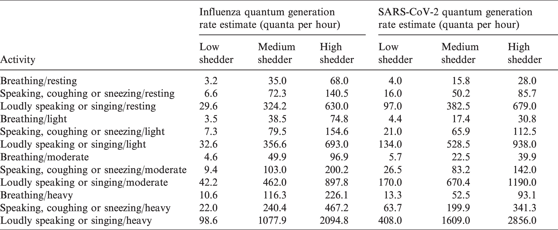
This model varies the quanta per hour by selected activity level and expiratory event, for either influenza or SARS-CoV-2. Both activity level, primarily through breathing (or pulmonary ventilation) rates, and expiratory means (speaking, breathing, coughing, etc.) influence the initial size and quantity of the virus-containing droplets/aerosols, the varying concentration levels of virus particles within the droplets/aerosols, the potential for a non-infected individual to breathe them in and the potential that they will reach deep enough in the lungs to cause an infection. Therefore, they impact the quantum of infection value.

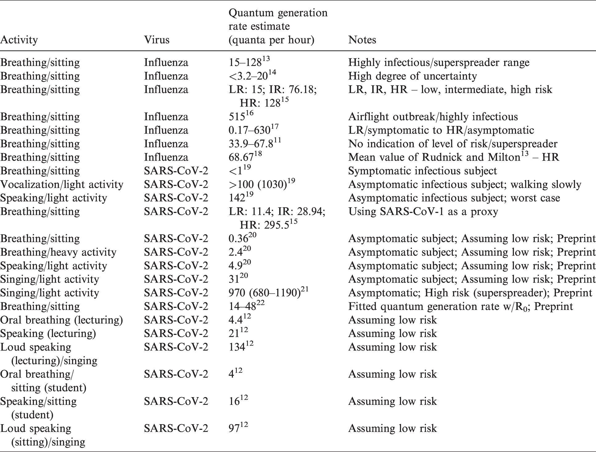
Table 1 lists the quantum generation rates by expiratory means/activity level for both influenza and SARS-CoV-2 that are used in this model. In addition, separate values are provided for low, medium and high shedders. These values are taken directly from and/or estimated from the values and sources listed in Table 2 as well as the Airborne Infection Risk Calculator manual. ¹⁰ Due to conflicting data and opinions in the research relative to varying quantum generation rates between adults and children,^11,12 the model currently assumes the same rate for both children and adults.

Table 1.

Quantum generation rate estimate (quanta per hour).

Activity	Influenza quantum generation rate estimate (quanta per hour)			SARS-CoV-2 quantum generation rate estimate (quanta per hour)
	Low shedder	Medium shedder	High shedder	Low shedder	Medium shedder	High shedder
Breathing/resting	3.2	35.0	68.0	4.0	15.8	28.0
Speaking, coughing or sneezing/resting	6.6	72.3	140.5	16.0	50.2	85.7
Loudly speaking or singing/resting	29.6	324.2	630.0	97.0	382.5	679.0
Breathing/light	3.5	38.5	74.8	4.4	17.4	30.8
Speaking, coughing or sneezing/light	7.3	79.5	154.6	21.0	65.9	112.5
Loudly speaking or singing/light	32.6	356.6	693.0	134.0	528.5	938.0
Breathing/moderate	4.6	49.9	96.9	5.7	22.5	39.9
Speaking, coughing or sneezing/moderate	9.4	103.0	200.2	26.5	83.2	142.0
Loudly speaking or singing/moderate	42.2	462.0	897.8	170.0	670.4	1190.0
Breathing/heavy	10.6	116.3	226.1	13.3	52.5	93.1
Speaking, coughing or sneezing/heavy	22.0	240.4	467.2	63.7	199.9	341.3
Loudly speaking or singing/heavy	98.6	1077.9	2094.8	408.0	1609.0	2856.0

Table 2.

Referenced quantum generation rate studies.

Activity	Virus	Quantum generation rate estimate (quanta per hour)	Notes
Breathing/sitting	Influenza	15–128 13	Highly infectious/superspreader range
Breathing/sitting	Influenza	<3.2–20 14	High degree of uncertainty
Breathing/sitting	Influenza	LR: 15; IR: 76.18; HR: 128 15	LR, IR, HR – low, intermediate, high risk
Breathing/sitting	Influenza	515 16	Airflight outbreak/highly infectious
Breathing/sitting	Influenza	0.17–630 17	LR/symptomatic to HR/asymptomatic
Breathing/sitting	Influenza	33.9–67.8 11	No indication of level of risk/superspreader
Breathing/sitting	Influenza	68.67 18	Mean value of Rudnick and Milton 13 – HR
Breathing/sitting	SARS-CoV-2	<1 19	Symptomatic infectious subject
Vocalization/light activity	SARS-CoV-2	>100 (1030) 19	Asymptomatic infectious subject; walking slowly
Speaking/light activity	SARS-CoV-2	142 19	Asymptomatic infectious subject; worst case
Breathing/sitting	SARS-CoV-2	LR: 11.4; IR: 28.94; HR: 295.5 15	Using SARS-CoV-1 as a proxy
Breathing/sitting	SARS-CoV-2	0.36 20	Asymptomatic subject; Assuming low risk; Preprint
Breathing/heavy activity	SARS-CoV-2	2.4 20	Asymptomatic subject; Assuming low risk; Preprint
Speaking/light activity	SARS-CoV-2	4.9 20	Asymptomatic subject; Assuming low risk; Preprint
Singing/light activity	SARS-CoV-2	31 20	Asymptomatic subject; Assuming low risk; Preprint
Singing/light activity	SARS-CoV-2	970 (680–1190) 21	Asymptomatic; High risk (superspreader); Preprint
Breathing/sitting	SARS-CoV-2	14–48 22	Fitted quantum generation rate w/R0; Preprint
Oral breathing (lecturing)	SARS-CoV-2	4.4 12	Assuming low risk
Speaking (lecturing)	SARS-CoV-2	21 12	Assuming low risk
Loud speaking (lecturing)/singing	SARS-CoV-2	134 12	Assuming low risk
Oral breathing/sitting (student)	SARS-CoV-2	4 12	Assuming low risk
Speaking/sitting (student)	SARS-CoV-2	16 12	Assuming low risk
Loud speaking (sitting)/singing	SARS-CoV-2	97 12	Assuming low risk

The model allows the user to select from the following expiratory means: Breathing, speaking, loudly speaking or singing, coughing and sneezing. These specific categories were used to coordinate the quanta generation by expiratory means with the droplet/aerosol size ranges produced by expiratory means (discussed below in the Settling removal factor section). The following activity levels are available to select from: resting (sitting, reading, sleeping and watching TV), light (standing and most domestic or office work), moderate (climbing stairs and light exercise) and heavy (vigorous exercise). These specific categories were used to coordinate the quanta generation by activity level with pulmonary ventilation rates, discussed further below.

Number of infected individuals

The model allows the option of selecting one or more infected individuals. Each infected individual is assumed to have the same expiratory means, activity level, quantum of infection and pulmonary ventilation rate.

Pulmonary ventilation (breathing)

Breathing rate is important to consider as it impacts the amount of virus potentially inhaled. It is also important to factor in the variation between adults and children. Adult and child pulmonary ventilation rates by activity level are determined using Table 6-31 from the EPA’s Exposure Factors Handbook. 23 The total daily IR (inhalation rate) value for an adult average, divided by 24 h, was used to provide the adult pulmonary ventilation rate for these calculations, representing ages 18 and older. The total daily IR value for a 10-year-old child, divided by 24 h, was used to provide the child pulmonary ventilation rate for these calculations, representing ages less than 18 years of age.

Table 3.

Initial and equilibrium droplet/aerosol weighted average GM by expiratory means.

Measurement range (μm)	Expiratory event	Droplet GM (μm) Calculated by the team	% Infectious droplets or % concentration	Calced droplet GM (μm)	% Infectious droplets or % concentration	Calced droplet GM (μm)	% Infectious droplets or % concentration	Calced droplet GM (μm)	% Infectious droplets or % concentration	Calced droplet GM (μm)	% Infectious droplets or % concentration	Weighted average GM (μm)	Equilibrium vs. initial	Estimated initial weighted average GM (μm)
0.3–unknown	Breathing	0.4	70%	0.7	17%	2.2	13%					0.7	Assumed equil.	1.4 14
0.3–10	Breathing	0.4	82%	2.2	18%							0.7	Assumed equil.	1.4 29
0.05–50	Breathing	0.2	90%	5.0	10%							0.7	Assumed equil.	1.3 30
0.5–20	Breathing	0.8	86%	1.8	9%	3.5	3%	5.5	2%			1.1	Assumed equil.	2.1 31
0.3–20	Breathing	0.6	64%	1.1	36%							0.7	Assumed equil.	1.5 32
Breathing Average												0.8		1.5
Breathing average, infected only												0.7		1.4
0.5–20	Speaking softly	0.8	85%	1.8	11%	3.5	3%	5.5	1%			1.0	Assumed equil.	2.1 31
0.5–20	Speaking normal	0.8	73%	1.8	21%	3.5	2%	5.5	4%			1.3	Assumed equil.	2.5 31
0.3–20	Speaking normal	0.5	79%	1.3	21%							0.7	Assumed equil.	1.3 32
0.3–20+	Speaking normal	0.8	43%	1.2	54%	145	3%					5.3	Equil.	10.7 33
0.3–20+	Speaking normal	0.8	44%	1.2	56%							1.0	Equil.	2.1 33
0.5–20	Speaking loudly	0.8	69%	1.8	13%	3.5	13%	5.5	5%			1.5	Assumed equil.	3.0 31
0.3–20	Speaking loudly	0.5	39%	1.3	61%							1.0	Assumed equil.	2.0 32
Speaking Normal Average w/ O-mode												2.4		4.8
Speaking normal average w/out O-mode												1.0		2.0
Speaking loudly average												1.3		2.5
0.3–20	Singing average	0.5	44%	1.1	56%							0.9	Assumed equil.	1.7 32
0.3–20	Singing loudly	0.6	34%	1.3	66%							1.0	Assumed equil.	2.1 32
Singing average												1.0		2.1
unknown	Cough	0.5	15%	1.7	25%	5.5	60%					3.8	Assumed equil.	7.6 9
unknown	Cough	0.5	35%	2.0	23%	6.3	42%					3.3	Assumed equil.	6.6 34
0.3–unknown	Cough	1.5	100%									1.5	Assumed equil.	3.1 35
0.5–20	Cough	0.8	83%	1.8	14%	3.5	2%	5.5	1%			1.0	Assumed equil.	2.1 31
0.3–20+	Cough	0.8	40%	0.8	54%	123.0	6%					8.1	Equil.	16.3 33
0.3–20+	Cough	0.8	43%	0.8	57%							0.8	Equil.	1.6 33
Coughing Average w/ O-mode												3.6		7.1
Coughing Average w/out O-mode												2.1		4.2
Coughing average, infected only												2.9		5.8
0.1–1000	Sneeze	Unimodal distribution; size class w/most droplets: 341.5–398.1 µm										360.1	Assumed initial	NA 36
0.1–1000	Sneeze	Bimodal distribution; size class w/most droplets: 73.6–85.8 µm										74.4	Assumed initial	NA 36
unknown	Sneeze	1.4	3%	2.8	16%	5.7	35%	11.3	28%	126.5	19%	29.0	Assumed initial	NA 37
	Sneezing Average											154.5		NA
	Sneezing average, excluding unimodal distribution											51.7		NA

Table 4.

Respiratory droplet/aerosol size transformation average D_eq/D_i ratios.

RH	Model-based Deq/Di ratios			Experimentally derived Deq/Di ratios	Average Deq/Di ratios
	Di = 0.1 μm	Di = 1.0 μm	Di = 10.0 μm
10%	0.401	0.402	0.402	0.391	0.399
20%	0.407	0.407	0.407	0.395	0.404
30%	0.412	0.412	0.412	0.398	0.409
40%	0.416	0.417	0.417	0.401	0.413
50%	0.422	0.423	0.424	0.427	0.424
60%	0.429	0.431	0.432	0.437	0.432
70%	0.439	0.443	0.444	0.449	0.444
80%	0.456	0.464	0.465	0.464	0.462
90%	0.49	0.513	0.516	0.502	0.505

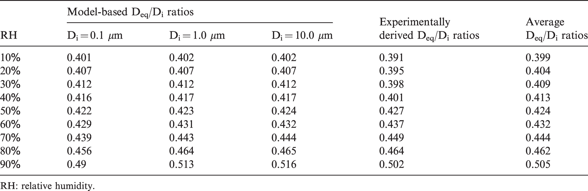
RH: relative humidity.

Table 5.

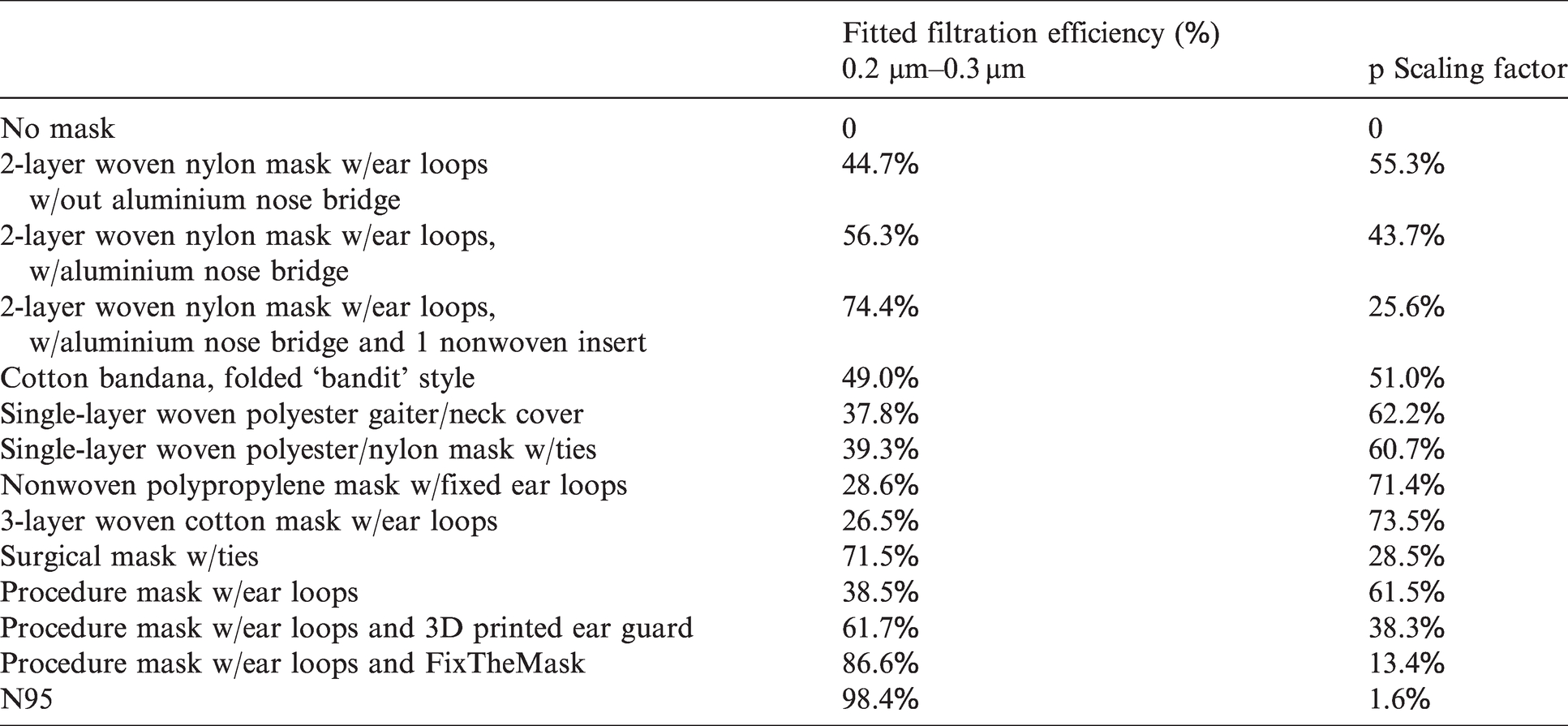
Filtration efficiencies and p scaling factor for masks used in this model ⁵³ .

	Fitted filtration efficiency (%)	p Scaling factor
	0.2 µm–0.3 µm
No mask	0	0
2-layer woven nylon mask w/ear loops w/out aluminium nose bridge	44.7%	55.3%
2-layer woven nylon mask w/ear loops, w/aluminium nose bridge	56.3%	43.7%
2-layer woven nylon mask w/ear loops, w/aluminium nose bridge and 1 nonwoven insert	74.4%	25.6%
Cotton bandana, folded ‘bandit’ style	49.0%	51.0%
Single-layer woven polyester gaiter/neck cover	37.8%	62.2%
Single-layer woven polyester/nylon mask w/ties	39.3%	60.7%
Nonwoven polypropylene mask w/fixed ear loops	28.6%	71.4%
3-layer woven cotton mask w/ear loops	26.5%	73.5%
Surgical mask w/ties	71.5%	28.5%
Procedure mask w/ear loops	38.5%	61.5%
Procedure mask w/ear loops and 3D printed ear guard	61.7%	38.3%
Procedure mask w/ear loops and FixTheMask	86.6%	13.4%
N95	98.4%	1.6%

Table 6.

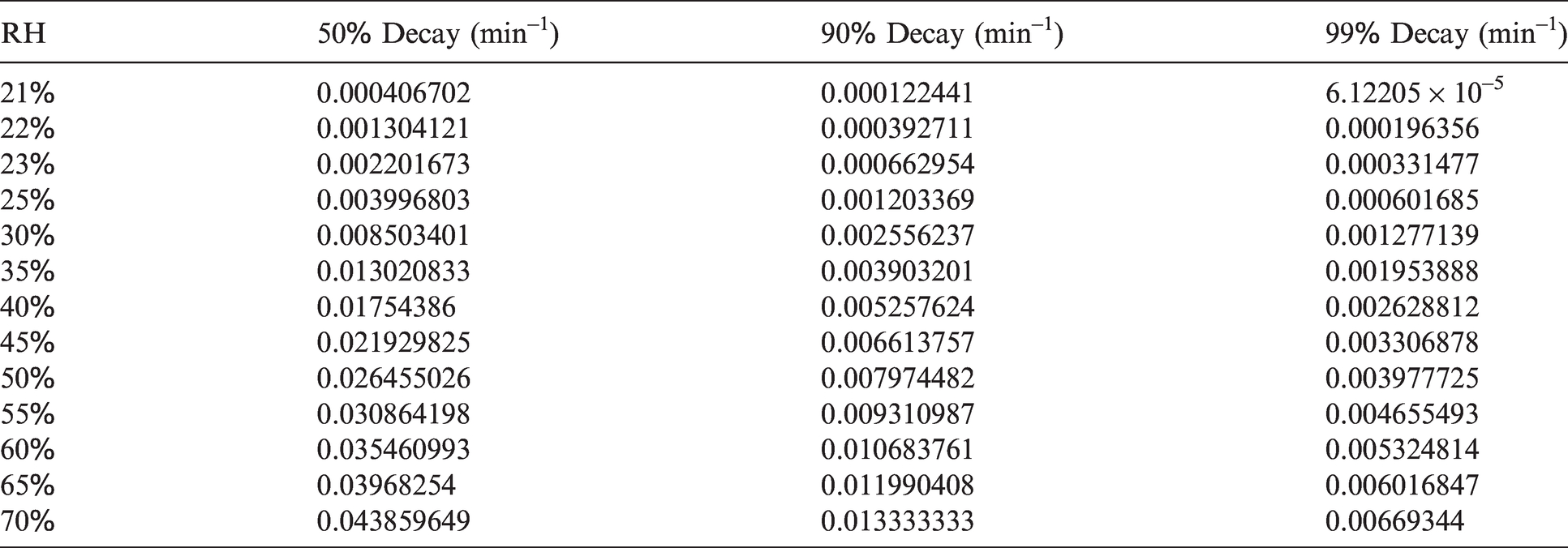
SARS-CoV-2 inactivation/decay rate (min⁻¹).

RH	50% Decay (min–1)	90% Decay (min–1)	99% Decay (min–1)
21%	0.000406702	0.000122441	6.12205 × 10–5
22%	0.001304121	0.000392711	0.000196356
23%	0.002201673	0.000662954	0.000331477
25%	0.003996803	0.001203369	0.000601685
30%	0.008503401	0.002556237	0.001277139
35%	0.013020833	0.003903201	0.001953888
40%	0.01754386	0.005257624	0.002628812
45%	0.021929825	0.006613757	0.003306878
50%	0.026455026	0.007974482	0.003977725
55%	0.030864198	0.009310987	0.004655493
60%	0.035460993	0.010683761	0.005324814
65%	0.03968254	0.011990408	0.006016847
70%	0.043859649	0.013333333	0.00669344

Modified p scaling factor (masks)

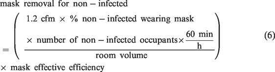
The mask effective efficiency value, discussed further below in the Removal and inactivation factors section, is used to calculate a scaling factor that scales the rate at which quanta of infection are breathed in as a result of wearing a mask. ²⁴ This is described by equation (2)

$$\begin{array}{l}\mathrm{modified}\mathrm{p}\mathrm{scaling}\mathrm{factor}(\mathrm{s})=\\ 1-(\mathrm{mask}\mathrm{effective}\mathrm{efficiency}\times \%\mathrm{\text{non-infected}}\mathrm{wearing}\mathrm{a}\mathrm{mask})\end{array}$$

(2)

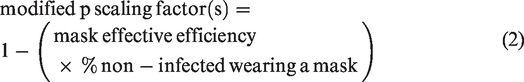
The unmodified p scaling factor (1 – mask effective efficiency) ²⁴ was modified to account for the potential that not all non-infected individuals are wearing a mask. The model allows one to input the percentage of infected and non-infected individuals wearing a mask. The unmodified p scaling factor values used for the different mask types are listed below in Table 5, discussed in the Removal and inactivation factors section.

Time of exposure

The model allows one to enter the time of exposure in hours. Exposure time will vary by (a) facility type, (b) the different occupants present in the facility and (c) the different activities they undertake during the day. For example, if an infected individual is present in a room, the exposure time of elementary students could be significantly more than an office worker meeting with an infected coworker for 20 min in a conference room.

Removal and inactivation factors

Research indicates aerosol transmission is likely a predominant route for the transmission of many viruses,^8,25,26 including influenza and SARS-CoV-2. Reducing the threat from virus-containing aerosols indoors, once the virus particles have been expirated from an infected person, is accomplished by removing or inactivating them before non-infected individuals have an opportunity to inhale them. The removal and inactivation mechanisms addressed in this model include settling (via gravity), ventilation (via outdoor air), filtration (via the building heating, ventilation, and air conditioning (HVAC) system, portable air cleaners and/or mask wearing) and virus inactivation (via RH and/or upper room UVGI). Each of these is discussed in more detail below.

Settling removal factor

Environmental conditions impact the rate of settlement due to gravity. Air flow may keep smaller droplets/aerosols in the air longer, and RH plays a large role in the size of the droplets/aerosols after leaving the infected host.^26,27 Droplets evaporate faster at lower RH levels, increasing their likelihood of staying aloft longer. Temperature also affects settling velocity through its impact on the dynamic viscosity of air; the warmer the temperature the higher the dynamic viscosity and the slower the settling velocity. As the dynamic viscosity of air does not vary significantly over the narrow temperature setpoint range found in most occupied spaces (68°F–76°F (20°C–24.4°C)), ²⁸ the dynamic viscosity for a temperature of 72.5°F (22.5°C) at one atmosphere of pressure is used for this model.

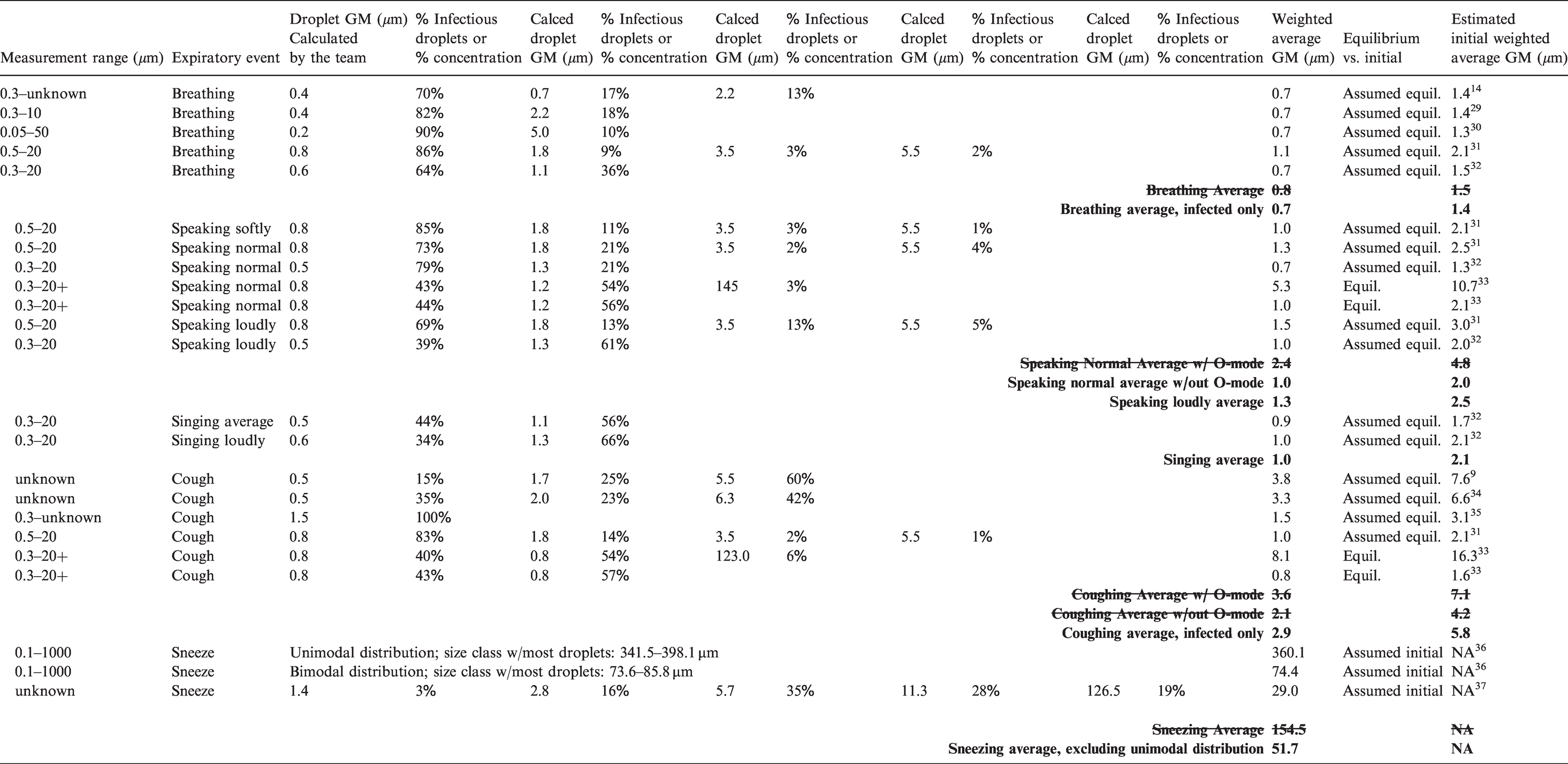
The means of expiration must also be considered because they impact the quantity and size of virus-containing droplets/aerosols that are released from an infected individual. This model uses a weighted average initial diameter for these droplets/aerosols (immediately after expiration) to estimate the removal efficiency associated with settling and the associated impact on the probability of infection. Table 3 provides the average initial droplet/aerosol diameters used by this model for the following expiratory means: breathing, speaking normally, speaking loudly, singing, coughing and sneezing, based on the references listed.

The table lists different measured droplet/aerosol (particle) diameter ranges (first column) associated with a specific expiratory means (second column) pulled from the various studies referenced in the last column. Within that overall range, as provided by the studies, the subsequent series of paired columns list (a) calculated GMs (geometric mean diameters) for various bins of particle size ranges and (b) an associated percentage. This percentage consists of either (a) the percentage of infectious particles within the bin relative to the infectious particles from the overall particle size range or (b) the percentage concentration of particles within the bin relative to the concentration of particles from the overall particle size range. For the referenced studies where it was possible, these series of paired columns are used to calculate the weighted average GM (third column from the end) using the following method. ⁹ The percentages of infectious particles contained within each associated bin of droplet/aerosol (particle) distribution ranges were multiplied by the GM from each of these bins, and then these products added together to obtain the weighted average GM for each referenced study.

However, because only a few studies involved infected volunteers, additional studies involving healthy individuals also had to be referenced. In these cases, the percentage concentration for each bin of droplet/aerosol size ranges as opposed to the percentage of infectious particles contained within each bin was used to determine the weighted average GM. Most of the studies reported equilibrium sizes for the droplet/aerosol size ranges (or were assumed to), which are the size of droplets/aerosols after reaching equilibrium with environmental conditions, primarily driven by RH. ³⁸ To estimate the initial weighted average GM (the last column), the equilibrium sizes were divided by an evaporation factor of 0.5. ³³

For each expiratory means, the size values from the relevant studies were averaged together to reach the final weighted average values used by the model. Where possible, the final selected average was determined from studies making use of only infected individuals. O-mode size distribution ranges were excluded due to available research suggesting greater concentrations of viral particles occur in smaller droplets/aerosols.^{14,27,30,31,34,35,39–41} These and other averages discarded for use in the model are crossed out in the table. In order to coordinate with the quanta generation by expiratory means (discussed above), speaking loudly and singing were combined into a single expiratory event, using the initial droplet/aerosol diameters for speaking loudly.

To calculate the settling removal efficiency (E_settling), the initial and equilibrium droplet/aerosol diameters are needed. As discussed above, Table 3 provides the average initial droplet/aerosol diameters used by this model. Equilibrium particle diameters were then calculated using an average of the model-based and experimentally derived respiratory droplet size transformation ratios (the last column in Table 4) that corresponds to the relevant room RH, shown in Table 4. ³⁸

Settling velocities were calculated referencing particle densities ⁴² and the Stokes Law formula ³⁸ ; v = (g × D_eq × ⍴)/(18 × μ); g = gravitational acceleration, ⍴ = particle density, μ = dynamic viscosity of air. The final formula for k_settling is equation (3)

$${\mathrm{k}}_{\mathrm{settling}}=\mathrm{v}/\mathrm{H}$$

(3)

v = settling velocity

H = height of the room/space.

Ventilation removal factor

Ventilation refers to the introduction of outside air (OA) into a space. It has the impact of diluting contaminants, including virus-containing aerosols, which in turn increases the amount of time required to inhale an infectious dose of virus. The continued introduction of OA also displaces the same amount of air within the space, removing contaminants in the process, though due to mixing it is not an immediate one-to-one replacement.^8,27,43

Ventilation may be supplied mechanically through HVAC systems or naturally through operable windows or other intentional or unintentional openings in the building envelope. Recommended ventilation rates will vary depending on factors such as the space or facility type, the activities being conducted, and the density of people present. Ventilation removal efficiency (E_ventilation) is dependent on ventilation rates for the room/space in question and entered as the total OA in cubic feet per minute (cfm) or cubic metre per hour in SI unit. k_ventilation equates to the OA changes per hour for the room/space, calculated using the entered OA per space and the space volume. Design ventilation rates are often not readily available unless one has access to as-built drawings and actual ventilation rates will often vary from design ventilation rates. Engineers, commissioning agents, and/or test and balance (TAB) consultants may need to be consulted to verify actual ventilation rates or determine a close approximation.

Filtration removal factor – Filters inside building systems

Filtration refers to a physical medium used to ‘capture’ contaminants, including droplets/aerosols, from the air as it passes through the medium. For building systems, filters follow a minimum efficiency reporting value (MERV) rating system, with values ranging from 1 on the low end all the way up to 16. The ratings provide an indication of how effective a filter is at removing particles of varying size ranges out of the air.^8,9,44 Filtration is effective if (a) the contaminants are airborne, such as virus-containing aerosols and (b) the clean air delivery is high enough.^8,9,45–47 Clean air delivery is a function of the filter’s efficiency and the recirculated air (RA) rate.

The building system filter removal efficiency (η_filter) percentages for various MERV and high efficiency particulate air (HEPA) ratings used are taken from aerosol-weighted values given in another source’s Table 4. ⁹ The available MERV and HEPA input selections are limited to the levels used in this table. Users must select the value closest to their existing and/or proposed conditions. Recirculated air changes per hour (λ_{recirculation}), entered as CFM per space, are needed to calculate the overall filtration removal efficiency (E_filtration). The final formula for k_filtration is equation (4)

$${\mathrm{k}}_{\mathrm{filtration}}={\mathrm{\lambda }}_{\mathrm{recirculation}}\times {\mathrm{\eta }}_{\mathrm{filter}}$$

(4)

λ_{recirculation} = recirculated air changes per hour for the room/space

η_filter = building system filter removal efficiency.

As with ventilation rates, engineers, commissioning agents and/or TAB consultants may need to be consulted to determine what filter rating and RA rate should be used.

Filtration removal factor – Portable air cleaners

Portable air cleaners are also available for use to supplement building system filtration and ventilation. Units sold in the U.S. should have a clean air delivery rate (CADR) corresponding to a recommended room volume. This model requires entering the CADR value of the unit(s) being used, and these ratings are typically provided by the manufacturer for smoke, dust and pollen. Some research^{14,30,34,48,49} suggests that a greater percentage of infectious viral particles (approximate 60% to over 90% for the studies referenced) are found in smaller droplets/aerosols, potentially 5 µm or less in diameter. This droplet/aerosol size range is more reflective of smoke and dust than pollen, ⁵⁰ therefore this model requires the average of the smoke and dust CADR rating be entered.

The removal rate per portable air cleaner, λ_aircleaner, equals the CADR value from the manufacturer divided by the space volume (V), ⁵⁰ as shown in equation (5)

$${\mathrm{\lambda }}_{\mathrm{aircleaner}}=\mathrm{CADR}/\mathrm{V}$$

(5)

This value is then multiplied by the number of portable air cleaners being used per space to provide the total removal rate (1/h).

Filtration removal factor – Masks

The last type of filtration accounted for by this model are masks, which block large droplets and filter a percentage of virus-containing aerosols from the air exhaled by an infected individual as well as from the surrounding air before they are inhaled by a non-infected individual.^30,51 The efficiency of a mask, or the percentage of aerosols with virus particles filtered out, depends on (a) the removal efficiency of the mask material itself relative to the different size distributions of droplets/aerosols and flow rate through the mask and (b) the leakage that occurs around the mask edges.^24,52–58

Leakage is largely related to how well the mask fits a person. The pressure drop across the mask material also impacts its usability as the greater the pressure drop, the harder it is to breathe through. Greater pressure drops may also result in greater leakage rates, especially if the fit is poor because more particles will follow the path of least resistance through the gaps between the face and mask. The mask removal efficiency (E_mask) is calculated looking at the following two components, added together.

Mask removal efficiency, part 1: This part consists of the amount of droplets/aerosols removed from the room air by the masks of the non-infected individuals as they breath in (equation 6 below) and is a small contribution compared to part 2. It is calculated using the mask effective efficiency (η_mask), the number of non-infected individuals wearing them, and the estimated breathing generated air change rate across an individual mask of 1.2 cfm (2.0 m³/h), ⁵⁵ as shown in equation 6.

$$\mathrm{mask}\mathrm{ }\mathrm{removal}\mathrm{ }\mathrm{for}\mathrm{ }\mathrm{non}-\mathrm{infected}=\left( \frac{1.2\mathrm{ }\mathrm{cfm}\mathrm{ }\text{×}\mathrm{ }\mathrm{\%}\mathrm{ }\mathrm{non}-\mathrm{infected}\mathrm{ }\mathrm{wearing}\mathrm{ }\mathrm{mask}\mathrm{ }\text{×}\mathrm{ }\mathrm{number}\mathrm{ }\mathrm{of}\mathrm{ }\mathrm{non}-\mathrm{infected}\mathrm{ }\mathrm{occupants}\text{×}\frac{60\mathrm{ }\min }{\mathrm{h}}}{\mathrm{ }\mathrm{room}\mathrm{ }\mathrm{volume}}\right)\text{×} \mathrm{mask}\mathrm{ }\mathrm{effective}\mathrm{ }\mathrm{efficiency}$$

(6)

The estimated breathing generated air change rate used here represents respiration rates at rest. This model uses Mask Effective Efficiency (η_mask) values shown in Table 5 (labelled fitted filtration efficiency (%)). These come from a study ⁵³ that directly measured the fitted filtration efficiency (FEE), accounting for both mask efficiency and face seal leakage, or mask fit.

In this study, the FixTheMask add on consisted of a rubber band configuration mimicking the impacts of the FixTheMask mask fitter, resulting in a measured FFE of 78.2%. Another study ⁵⁹ actually tested the manufactured FixTheMask mask fitter on a procedure mask using a similar particle range as the above study, though manikins were used instead of an actual person. The effective mask efficiency, or FEE, was found to be 94.9%. For the model, these two values were averaged, giving an FFE of 86.6%.

Mask removal efficiency, part 2: This part consists of the amount of droplets/aerosols removed by the masks from the air breathed out by the infected individual(s), before they enter the room air, as shown in equation (7)

$$\mathrm{ }\mathrm{source}\mathrm{ }\mathrm{reduction}=\left(\mathrm{mask}\mathrm{ }\mathrm{effective}\mathrm{ }\mathrm{efficiency}\mathrm{ }\text{×}\mathrm{ }\mathrm{\%}\mathrm{ }\mathrm{infected}\mathrm{ }\mathrm{wearing}\mathrm{ }\mathrm{a}\mathrm{ }\mathrm{mask}\right)$$

(7)

The final formula for k_mask is then equation (8)

$${\mathrm{k}}_{\text{mask}}=(\mathrm{mask}\mathrm{ }\mathrm{removal}\mathrm{ }\mathrm{for}\mathrm{ }\mathrm{non}-\mathrm{infected}\mathrm{ }+\mathrm{ }\mathrm{source}\mathrm{ }\mathrm{reduction})$$

(8)

Inactivation – RH removal factor

Inactivation refers to a process of rendering a virus non-infectious. This model focuses on two types of inactivation. The first is in relation to RH, as research indicates that for typical interior temperature ranges, most viruses, including membrane-bound viruses like SARS-CoV-2 and influenza, find low (< 40%) and high (>90%) RH levels more conducive to survival with increased decay rates occurring at intermediate RH levels.^{25,27,60–62} As droplets/aerosols evaporate after expiration, the concentration levels of proteins, salts, etc., within them increase, creating conditions unfavourable to the virus and likely speeding up its inactivation, though additional research is needed to understand the nuances of how this varies by virus type, strain, phenotypic characteristics, temperature and specific respiratory fluid characteristics. For the purposes of this model, a linear relationship was assumed for influenza ²⁷ and SARS-CoV-2. ⁶³

While temperature impacts virus inactivation, ²⁵ there does not appear to be any significant variation in virus decay over the narrow temperature setpoint range found in most occupied spaces, 68°F–76°F (20°C–24.4°C). ²⁷ For the purposes of the model, an interior temperature of 22.5°C (72.5°F) and associated dynamic viscosity of air of 1.83 × 10⁻⁵ was assumed. For SARS-CoV-2, an interior temperature of 72°F (22.2°C) was assumed to coordinate the constraints of the Department of Homeland Security calculator ⁶³ used to estimate the virus’ inactivation due to RH (discussed further below). These assumptions also coordinate with the interior temperature assumptions made for settling discussed above.

The influenza A virus inactivation rate (k_{RHinactivationIVA}) due to RH entered was calculated using equation (9) ³⁸

$${\mathrm{k}}_{\mathrm{RHinactivationIVA}}=(0.0438\times \mathrm{RH})-0.00629$$

(9)

For SARS-CoV-2, the inactivation rate (k_{RHinactivationSC2}) was calculated using equation (10)

$${\mathrm{k}}_{\mathrm{RHinactivationSC2}}=(0.0135\times \mathrm{RH})-0.0028$$

(10)

The equation was developed using a web application developed by the Department of Homeland Security. ⁶³ Decay rates were determined using this calculator for a UV Index of 0 (inside) and an interior assumed temperature of 72°F (22.2°C) to correspond to assumptions made for influenza and droplet evaporation. Note that the Department of Homeland Security calculator only provided values between a RH of 20+% and 70%. Table 6 then converts these values to 1/min, which were then graphed and equation (10) formulated for the 99% decay rate values.

Inactivation – Upper room UVGI removal factor

The second type of inactivation focused on in this model is upper room UVGI. A sufficient dosage of UV radiation will inactivate viruses (by photochemical disruption of viral RNA upon absorbing UV photons), with the ultraviolet C (UV-C) band of energy (wavelengths between 100 and 280 nm) having the greatest germicidal effect.^43,64–66 Upper room applications of this technology make use of UV radiation generating lamp sources (low/medium pressure mercury vapour lamps or UV-C - LEDs), either wall mounted or suspended from the ceiling, to irradiate upper air zones of individual spaces while shielding the lower occupied zones from harmful UV radiation.^65–70 Substantial evidence exists for the effectiveness of upper room UVGI systems in killing various pathogens, including coronaviruses.^46,71

Germicidal effectiveness of these systems is influenced by spatial configuration, the location, number and power of the UV fixtures, RH, the airflow and air mixing that occurs between the lower occupied zone and upper irradiated zone, and the type of pathogen and its source(s). Of all these influences, the air up flow rate perhaps has the most impact, as this determines the speed with which pathogens are carried up into the irradiated zone to be eliminated, as well as how long they are irradiated, impacting the dose received. However, this simplified model assumes a well-mixed condition and only indirectly accounts for the impact of the airflow rate and air changes per hour ACH (discussed further below).

The upper room UVGI coefficient of inactivation (or removal factor) was calculated by multiplying the UVGI system’s upper room average irradiance or fluency (E) by the relevant susceptibility parameter (Z) for either influenza or SARS-CoV-2,^{65–69,72–76} as shown in equation (11)

$$[{\text{k}}_{\text{UVGIinactivationIVA}}{\text{or k}}_{\text{UVGIinactivationSC}2}]=\mathrm{E}\times \mathrm{Z}$$

(11)

Sources, including the 2009 NIOSH application guideline, recommend that the upper room average irradiance (E) should generally fall within the range of 30–50 µW/cm² for most pathogens.^66,74

However, the final average value depends on the number of lamps, their individual output, fixture configuration, fixture layout and room parameters. Measured and modelled values often fall below this range.^66,69,74 It will likely be necessary to coordinate with a design engineer and/or manufacturer to determine an appropriate estimate for a given setting. For these calculations, the effective average irradiance (E) for the whole space was used instead of the upper room average irradiance and was estimated by multiplying the upper room average irradiance by the ratio of upper room volume to total room volume.^74,77 Under well-mixed conditions (obtained via ceiling fans, the building mechanical system or some combination), some research ⁷⁷ indicates the whole room average irradiance value adequately accounts for the effects of air turnover rates between the upper and lower zones for all fan speeds of conventional low-velocity ceiling fans. However, potential conditions of either stagnation or greater than six ACH ⁴³ will likely result in the model overestimating the effectiveness of the upper room UVGI system.

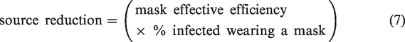
Reported susceptibility parameter (Z), or UV rate constant, values (m²/J) for influenza A include 0.15, ⁷² 0.27, ⁷⁸ 0.29 at 25–27% RH, ⁷³ 0.27 at 50–54% RH ⁷³ and 0.22 at 81–84% RH. ⁷³ In order to tie the Z value to RH, the last three values were used; see Table 7. The second RH range column was added to tie it to the RH ranges accounted for by this model.

Table 7.

Estimated Z values for influenza aerosols determined at low, medium and high relative humidity (modified from Table 1 ⁷³ ).

RH range (%)	RH range (%)	Estimated Z value (m2/J)	95% confidence interval		R2
			Lower	Upper
25–27	0%–33%	0.29	0.27	0.31	0.985
50–54	34%–66%	0.27	0.26	0.31	0.991
81–84	67%–100%	0.22	0.21	0.23	0.992

Reported susceptibility parameter (Z), or UV rate constant, values (m²/J) for SARS-CoV-2 include the suggestion ¹⁶ for 0.377 (best-case) and 0.0377 m²/J (worst-case) and the suggestion ⁷¹ of 0.05524 m²/J. At this point, there are no known studies linking the susceptibility parameter (Z) for SARS-CoV-2 to RH, so for the purposes of this model, the average of 0.377 and 0.0377 m²/J was used (0.207 m²/J).

The relationship between ACH, ventilation and UVGI is not fully understood. ²⁴ Greater ACH levels within lower ranges can positively impact room mixing, aiding in UVGI’s effectiveness by increasing the percentage of pathogens exposed at a faster rate. However, greater ACH rates also decrease its effectiveness relative to delivered dosage by decreasing the amount of exposure time for the pathogens in question. Future versions may look at incorporating these parameters, but for now the effective average irradiance for the whole space was used to partially account for not directly estimating the impacts of ACH or air turnover rates on delivered dosage, as discussed above.

Adjusted vaccination factor

The model also accounts for the impacts of vaccination for influenza. Default influenza U.S. coverage rates for children (57%) and adults (42%) are provided based on averages of nine consecutive flu seasons for each, calculated from data provided by the Centers for Disease Control and Prevention. ⁷⁹ However, users of the model may modify these default values if desired. As COVID vaccinations are still rolling out and yet to be approved for children under 12 (as of this paper’s publication), local vaccination percentages are recommended to be used to guide the input for the percentage of adults and children 12 and over who are vaccinated.

To integrate the impact of vaccination into these calculations, the relationship between the probability of infection calculated by this model and the basic reproduction number, R₀ is used. R₀ is ‘… defined as the expected number of secondary cases produced by a single (typical) infection in a completely susceptible population’, ⁸⁰ and the probability of infection is one of three factors multiplied by each other to calculate R₀.

The impact of vaccination on the reproduction number can be estimated using equation (12)

$${\mathrm{R}}_{0\mathrm{p}}=(1-\mathrm{p})\ast {\mathrm{R}}_0$$

(12)

‘where R_0p is the R₀ under vaccination and p is the vaccination coverage rate of the population who have been vaccinated’. ¹¹ This model uses the relationship between R₀ and the probability of infection to estimate the impact of vaccination on the probability of infection, essentially multiplying it by (1–p). As vaccinations are not 100% effective, the p value for children and adults is also multiplied by estimates of influenza vaccination effectiveness for children (0.70) and adults (0.62). ⁸¹ This provides the adjusted vaccination factor (v_adjusted) applicable for influenza.

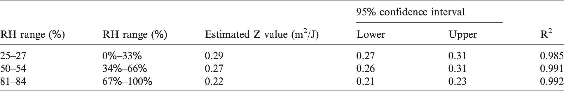
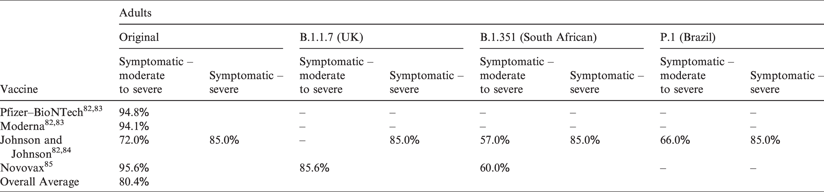
For SARS-CoV-2, adult efficacy percentages for the most prominent vaccines are listed in Table 8 (also used as a proxy for those 12 to 15 years of age as of this paper’s publication). These have been obtained from the sources listed for each vaccine. As indicated in the table, the efficacies for Johnson and Johnson were determined for both moderate to severe and severe symptoms. Cells with dashes indicate no formal efficacy values are available at this point. However, preliminary data does indicate the efficacy of the Pfizer and Moderna vaccines may be less for some of the variants. Due to limited data and uncertainty regarding the variants, it was decided to use one estimated efficacy value, averaging all of the percentages listed in Table 8 together, resulting in a value of 0.80. As more efficacy data become available, the model will be updated. The model currently does not allow one to account for any immunity generated through previous community infections. In those cases where a large number of such individuals (who are also unvaccinated) may be present within a building population, the results will overestimate the probability of infection to an unknown degree.

Table 8.

SARS-CoV-2 vaccine efficacy.

Vaccine	Adults
	Original		B.1.1.7 (UK)		B.1.351 (South African)		P.1 (Brazil)
	Symptomatic – moderate to severe	Symptomatic – severe	Symptomatic – moderate to severe	Symptomatic – severe	Symptomatic – moderate to severe	Symptomatic – severe	Symptomatic – moderate to severe	Symptomatic – severe
Pfizer–BioNTech82,83	94.8%		–	–	–	–	–	–
Moderna82,83	94.1%		–	–	–	–	–	–
Johnson and Johnson82,84	72.0%	85.0%	–	85.0%	57.0%	85.0%	66.0%	85.0%
Novovax 85	95.6%		85.6%		60.0%		–	–
Overall Average	80.4%

Validation of model against previous infection cases

To demonstrate the strengths and weaknesses of the web application ¹ and its underlying model, it has been used to model the outcomes of two documented superspreading events: the Skagit Valley chorale superspreading event ²¹ and the Guangzhou restaurant event.^86–88

Skagit Valley chorale superspreading event

In March 2021, a COVID-19 outbreak occurred as the result of a choral practice at the Mount Vernon Presbyterian Church in Skagit Valley, Washington, U.S. One symptomatic individual attended the choral practice which included a total of 61 vocalists. After the practice, 53 members were confirmed through testing or were strongly suspected of as having contracted COVID-19 from reported symptoms. A detailed analysis of this likely superspreading event was previously performed, ²¹ assuming transmission was predominantly via virus-containing aerosols and using gathered data to infer the quanta generation rate of aerosols emitted by the infected individual. Based on this previous analysis and data gathered to perform it, the following parameters were entered into the model.

Rehearsal hall room size: 1937.5 ft² (180 m²), 14.76 ft (4.5 m) ceiling. ²¹

Design OA: 1236 cfm (2100 m³/h). The referenced analysis ²¹ used ASHRAE Standard 62.1 and existing mechanical drawings to estimate the design ventilation, or OA, for the rehearsal hall.

Design RA: 3473 cfm (5900 m³/h). The referenced analysis ²¹ used ASHRAE Standard 62.1 and existing mechanical drawings to estimate the design RA for the rehearsal hall.

Choir practice OA: 334 cfm (567 m³/h), ±50% uncertainty: 167 cfm (284 m³/h)–501 cfm (850 m³/h). Based on the data gathered, the referenced analysis ²¹ assumed the HVAC fan was not operating during the choir practice, providing no mechanical outside or RA (the body heat from the number of choir members present was sufficient to maintain a comfortable temperature). Based on the delta between exterior and interior temperatures during the practice, the estimated body heat generated by individual choir members and the heat capacity of air, an estimate was made by the referenced analysis ²¹ of the amount of OA that entered via infiltration, along with values representative of ±50% uncertainty.

Choir practice RA: 0 cfm (0 m³/h). ²¹ The system was not running at the time of the event.

Furnace filter: MERV 11. ²¹

Temperature: Thermostat setting: 68°F (20°C), assumed interior temperature: 71°F (22°C), determined from gathered data. ²¹ The interior temperature fits within the 68°F–76°F (20°C–24.4°C) that this model is currently optimized for.

Relative humidity (RH): 30% RH. No RH information for the rehearsal hall room during the practice was provided. ²¹ Nor was the use of any type of humidifier indicated. As the heater had been on to warm the space before choir members arrived, the air was assumed to be at a lower humidity than if the heater had not been running. Deviations from this estimation are discussed below.

Number of infected individuals: 1. The referenced analysis ²¹ made this estimation based on one choir member having ‘cold-like’ symptoms manifesting three days prior to the practice and subsequently testing positive for COVID-19.

Viral shedding level: High. Referencing other published analyses of COVID-19’s incubation time, the referenced analysis ²¹ estimates that such a high secondary attack rate resulting from one infected person would require high shedding of the virus by the infected individual.

Activity level: Light. Choral members were generally sitting while practicing with some limited standing and walking. ²¹ Holding music and singing while sitting would be more along the lines of office work as opposed to passively sitting while resting. Therefore, a ‘light’ activity level was selected, which would also encompass standing and leisurely walking for short distances.

Number of choral members present: 61. ²¹ This includes the infected individual.

Expiratory means/exposure time: The following breakdown was selected for this analysis. The probability of infection was calculated for each time period and the net probability of infection determined from these three individual values.

Singing/126 min (2.1 h)

Speaking/18 min (0.3 h)

Breathing only/6 min (0.1 h).

The total rehearsal time was determined to be 2.5 h, ²¹ broken up as follows:

Phase 1: 45 min with the 61 choral members all together in the Fellowship Hall. This time was spent primarily practicing with a brief amount of time transitioning to the next phase.

Phase 2: 45 min spent primarily practicing in two groups. Group 1 consisted of approximately 35 people practicing in the Fellowship Hall and group 2 consisted of approximately 26 people practicing in the sanctuary. The infected person was part of Group 1.

Break: 10 min with everyone talking and eating snacks.

Phase 3: 50 min with the 61 choral members practicing all together in the Fellowship Hall.

To simplify the analysis, Phase 2 was modelled as the same conditions in Phase 1. This was decided due to (a) lacking dimensional and ventilation information for the sanctuary and (b) the infected person being part of the group practicing in the Fellowship Hall. In addition, an average amount of time of singing vs. speaking vs. breathing over the 2.5 h was estimated referencing the answers provided by the choir spokesperson. ²¹

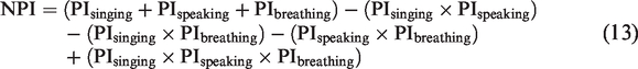
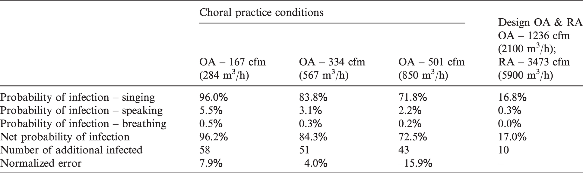
Table 9 provides (a) the resulting probability of infections calculated using this model, given the above estimations and (b) the potential resulting number of additional people infected, given the net probability of infection. The probability of infection for the three different expiratory means/exposure times is listed as well as the resulting net probability (the chance that at least one of these three conditions occurs). The net probability is calculated as shown in equation (13)

$$\begin{array}{l}\mathrm{NPI}=(\mathrm{P}{\mathrm{I}}_{\mathrm{singing}}+\mathrm{P}{\mathrm{I}}_{\mathrm{speaking}}+\mathrm{P}{\mathrm{I}}_{\mathrm{breathing}})-(\mathrm{P}{\mathrm{I}}_{\mathrm{singing}}\times \mathrm{P}{\mathrm{I}}_{\mathrm{speaking}})\\ -(\mathrm{P}{\mathrm{I}}_{\mathrm{singing}}\times \mathrm{P}{\mathrm{I}}_{\mathrm{breathing}})-(\mathrm{P}{\mathrm{I}}_{\mathrm{speaking}}\times \mathrm{P}{\mathrm{I}}_{\mathrm{breathing}})\\ +(\mathrm{P}{\mathrm{I}}_{\mathrm{singing}}\times \mathrm{P}{\mathrm{I}}_{\mathrm{speaking}}\times \mathrm{P}{\mathrm{I}}_{\mathrm{breathing}})\end{array}$$

(13)

Table 9.

Probability of infections and resulting additional choral members potentially infected.

	Choral practice conditions			Design OA & RA
	OA – 167 cfm (284 m3/h)	OA – 334 cfm (567 m3/h)	OA – 501 cfm (850 m3/h)	OA – 1236 cfm (2100 m3/h); RA – 3473 cfm (5900 m3/h)
Probability of infection – singing	96.0%	83.8%	71.8%	16.8%
Probability of infection – speaking	5.5%	3.1%	2.2%	0.3%
Probability of infection – breathing	0.5%	0.3%	0.2%	0.0%
Net probability of infection	96.2%	84.3%	72.5%	17.0%
Number of additional infected	58	51	43	10
Normalized error	7.9%	–4.0%	–15.9%	–

NPI = net probability of infection

PI_singing = probability of infection – singing

PI_speaking = probability of infection – speaking

PI_breathing = probability of infection – breathing.

The number of additional people infected is 60 uninfected individuals multiplied by the net probability of infection.

For the estimated ventilation of 334 cfm (567 m³/h), the resulting net probability of infection was estimated to be 84.3%, or an estimated 51 additional infected individuals. This is two less than the likely 53 additional choral members infected. Results are also provided for the ±50% uncertainty ventilation rates, giving potential numbers of additional infected individuals of 58 and 43 respectively for the low and high ventilation rates. The difference, or error, between the predicted and actual number of additional people infected, normalized by the total number of uninfected people initially present is also provided. This error was normalized using the total number of uninfected people initially present. In addition, for comparison purposes, results are also provided for the design ventilation and RA rates. If the furnace had been running, providing these design rates, the model estimates a net probability of infection of only 17%, or 10 additional people potentially infected.

The results provided in Table 9 are based on a RH of 30%, though it is possible the RH varied from this depending on how much the furnace dried the air out prior to the practice and how rapidly the RH subsequently increased after the furnace was shut off. To account for this, Figure 1 shows the potential number of additional people infected for 20% RH, 30% RH and 40% RH.

Figure 1.

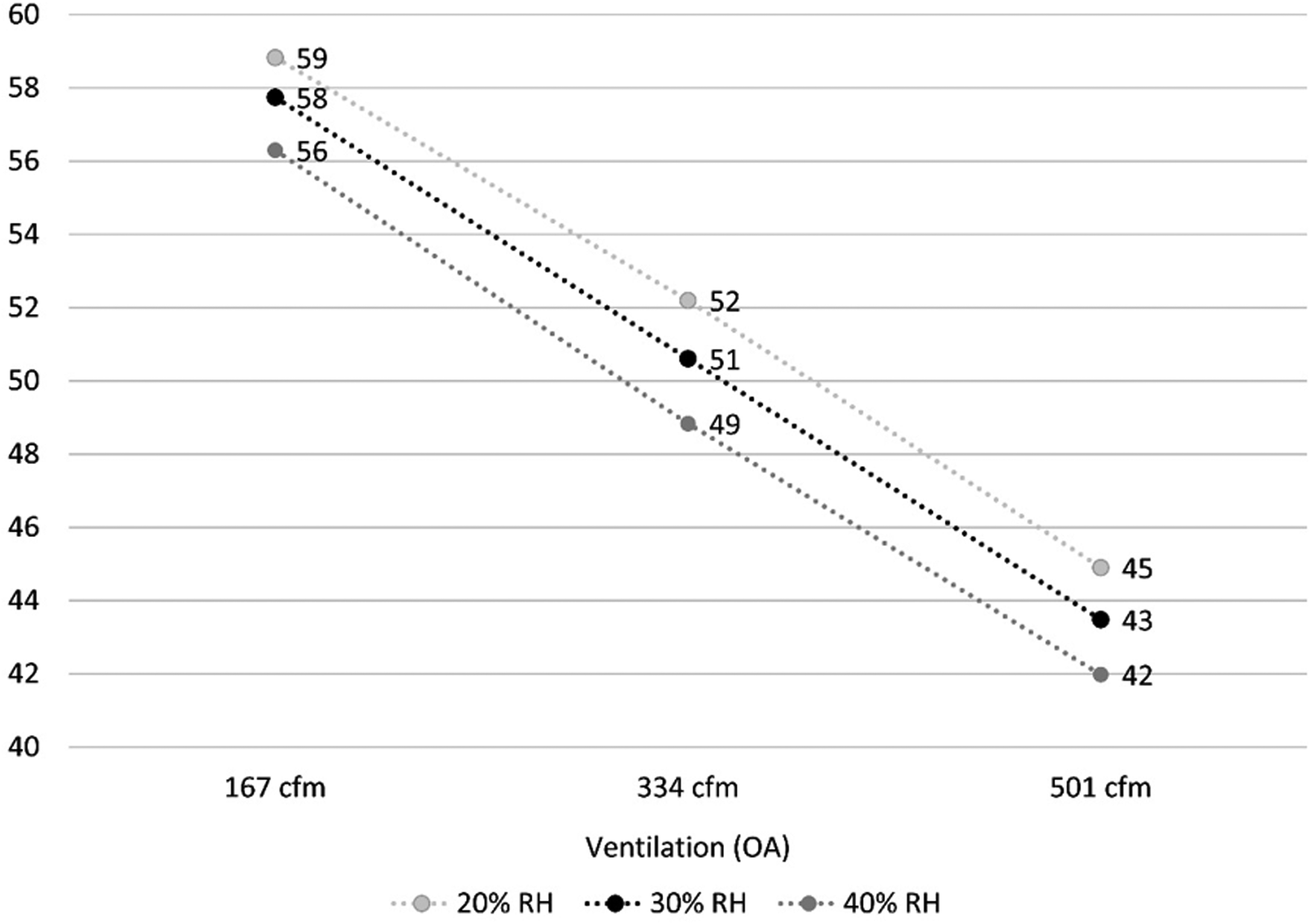
The potential number of additional people infected depending on ventilation and RH.

Depending on the actual choir practice ventilation rate and interior RH (ranging from 20% to 40%), the model’s normalized error output ranges in underestimating the probability of infection and resulting number of people potentially infected by 18.4% to overestimating them by 9.7%. If we assume that 334 cfm (567 m³/h) is very close to the actual choir practice ventilation rate, then the model’s normalized error output ranges in underestimating these values from 6.9% to 1.3%. So overall:

Normalized error range for all ventilation rates: –18.4% to 9.7%

Normalized error range for 334 cfm (567 m3/h) OA: –6.9% to –1.3%.

Guangzhou restaurant event

On 24 January 2020, a spreading event is thought to have occurred at an unnamed restaurant in Guangzhou, China.^86,87 It occurred on the third floor of the restaurant in question, where a single index case is thought to have infected nine additional patrons out of a total of 89 patrons present for between 53 and 75 min. Masks were not worn. Based on the associated epidemiological data, data gathered on the restaurant and its operations, as well as an analysis involving tracer gas and computer simulation, the following parameters were entered into the model.

Dining room size: The estimated area and ceiling heights were taken directly from the referenced analyses.^86,87 Scenario 1 examines the whole third floor dining area. Scenario 2 only looks at the air conditioning zone within which the infections occurred. No patrons outside of this particular zone ended up being infected. Within the dining room there are five ceiling mounted fan-coil air conditioning units located along one of the long walls, each serving a separate ‘zone’ within the room, with its own supply and return at the unit. While there are no physical barriers between the zones to prevent air mixing across the zones, the air flow from the supply out across the width of the room and then back to the return does limit some of the mixing. In addition, the zone in which the infections occurred was also at the far end of the room, further isolating it from the other zones. As this model assumes droplets/aerosols are instantaneously, continuously and evenly distributed throughout the room upon expiration, applying it to the whole dining space may be too great a simplification to accurately predict the probability of infection, given the limitations on air mixing between the zones. Therefore, an analysis is also run on the one zone only where the infections occurred. This results in the two scenarios being analysed.

Scenario 1: 1482.2 ft2 (137.7 m2), 10.3 ft (3.14 m) ceiling.

Scenario 2: 193.8 ft2 (18 m2), 10.3 ft (3.14 m) ceiling.

Ventilation OA: Ventilation in the space was apparently limited to brief, infrequent openings of the fire door and infiltration due to negative air pressure created by the restroom exhaust fan running. ⁸⁷ While the dining space had wall mounted exhaust fans to promote ventilation, they were turned off during the period in question. Also, the five fan-coil air conditioning units serving the dining space did not supply outdoor air – they are recirculating only units. Based on the tracer gas analysis, ⁸⁷ the ACH during the period in question was estimated to be between 0.56 and 0.77. These values along with the volume of the dining space for each scenario were used to determine the following cfm ranges:

Scenario 1: 142 cfm (242 m³/h)–196 cfm (333 m³/h)

Scenario 2: 18.6 cfm (31.7 m³/h)–25.6 cfm (43.5 m³/h).

Recirculated air (RA): Unfortunately, no detailed information on the fan-coil air conditioning units was provided. Based on the image in a letter response from one of the analyses, ⁸⁸ these appear to be cassette fan-coil units in a chilled water DX split system. To estimate the RA supplied by each unit, a design ventilation rate was first estimated using ASHRAE 62.1. Based on the square footage of the dining space, this rate is determined to be 1045 cfm (1776 m³/h) for the whole dining area. A rough rule of thumb is that ventilation air is 20% of the total supply air. As the RA is the total supply air minus the ventilation air. The RA was then estimated at 4180 cfm (7102 m³/h) using this rule of thumb.

The ESACIR horizontal concealed ceiling exposed cassette chilled water fan-coil unit, by Shenzhen Eurostars Technology Co., Ltd, ⁸⁹ is likely similar to the fan-coil unit depicted in the image referenced above. ⁸⁸ From the drawings/plans in one of the referenced analyses, ⁸⁷ there may have been two different sizes of units. Using the listed high air flow ratings for a 2-pipe system, (3) of the 1000HC2 units (1000 cfm/1700 m³/h) and (2) of the 600HC2 units (600 cfm/1020 m³/h) would satisfy the RA calculated above. As the speed these units were likely running at was not reported, the medium speed/airflow setting was decided for this analysis. As per the above drawings/plans, the air-flow zone where the infections occurred was served by one of the larger units. Therefore, the RA was estimated to be as follows for each scenario:

Scenario 1: 3161 cfm (5370 m³/h)

Scenario 2: 753 cfm (1280 m³/h).

Fan-coil unit filter: MERV 4 for both scenarios. For the ESACIR unit mentioned above, a washable filter is listed as optional. Such filters typically have a MERV rating of 1 to 4. Other similar cassette fan-coil units may accept disposable filters ranging in MERV ratings from 1 to 13, though ratings above 4 typically require the addition of a filter box. The image ⁸⁸ referenced above does not appear to include a filter box with the unit, so a filter with a MERV rating greater than 4 was unlikely to present. As a result of field measurements and computer simulations, the study ⁸⁷ reported a filtration efficiency of 20% for an aerosol diameter of 5 µm, which would suggest the presence of a MERV 4 or equivalent filter.^8,9 Each scenario is therefore run using a MERV 4 filter.

Temperature: No information was given on the interior temperature in any of the referenced analyses.^86–88 The interior temperature was assumed within the 68°F–76°F (20°C–24.4°C) that this model is currently optimized for.

Relative humidity (RH): 40% RH for both scenarios. No information was given on the RH in any of the referenced analyses.^86–88 As the air conditioning fan-coil units were running with very little OA provided, the RH humidity was assumed to have been lower than the exterior average 72% RH for this time of year in Guangzhou, somewhere between 30% and 50%. While the analysis could have been run for 30%, 40% and 50% RH values, based on the limited impact of RH within a similar range on the previous Skagit Valley chorale superspreading event analysis, the authors decided to focus only on 40% RH to simplify the analysis.

Number of infected individuals: One for both scenarios. As reported in the referenced analyses,^86,87 one infected individual sitting at the middle table of the air-flow zone in which all of the infections occurred served as the infected person.

Viral shedding level: High for both scenarios. This person was reported to have developed symptoms later that day, so this person appears to have been pre-symptomatic while dining in the restaurant. It has been reported that patients may be most infectious in the initial period after infection, before or shortly after symptoms emerge.^90–92 For these reasons, the authors of the study ⁸⁷ estimated that the index case had a ‘relative large quanta generation rate’ while dining. This study followed their lead and used the high shedder condition for the index case.

Activity level: Light. Sitting while talking and eating would be more along the lines of office work as opposed to passively sitting while resting. Therefore, a ‘light’ activity level was selected.

Number of patrons present: For the purposes of this analysis, waiters and other restaurant staff were excluded from the analysis, as they were not consistently present within the dining area. The study ⁸⁷ reported 89 patrons were present during the time in question, and that 21 patrons sat within the airflow zone in which the infections occurred. In addition, nine patrons were infected as a result of this incident, all sitting at the tables encompassed within scenario 2. No indication of adults vs. children among the patrons was provided, so it is assumed these are all adults. Therefore, the number of patrons for each scenario consists as follows:

Scenario 1: 89 patrons, including the single infected person and the nine additional infected individuals.

Scenario 2: 21 patrons, including the single infected person and the nine additional infected individuals.

Expiratory means/exposure time: The following breakdown was selected for this analysis. The probability of infection was calculated for each time period and the net probability of infection determined from these three individual values.

Speaking loudly: 6 min (0.1 h)

Speaking: 24 min (0.4 h)

Breathing (listening/eating/drinking): 36 min (0.6 h).

The time of exposure reported in the referenced analyses^86,87 was only for the three tables located in the airflow zone in which the infections occurred. Three families occupied these three tables at the following times – Table A: 12:01–13:23, Table B: 11:37–12:54 and Table C: 12:03–13:18. The infected person sat at Table A, overlapping with Table B by 53 min and with Table C by 75 min. Averaging the (2) times together results in 64 min, which is rounded up to 66 min to equate to an even 1.1 h of exposure time. The amount of time Table A overlapped with the remaining 68 patrons is unknown, so 1.1 h was used as an approximation.

Little information in the referenced analyses^86,87 is provided on the expiratory means, and these patrons were assumed to have spent their time in the restaurant breathing, eating/drinking, speaking and potentially speaking loudly. For the purposes of this analysis, breathing was assumed to expel a similar quantity and size distribution of virus-containing aerosols as eating/drinking, though this may underestimate the amount produced. Little research in general appears to exist quantifying the amount of a group mealtime spent eating/drinking vs. speaking vs. listening/breathing.

For the 66 min, the authors assumed that 24 min were spent speaking/listening and waiting for the food to be served, 30 min were spent eating/drinking and speaking/listening, and 12 min were spent speaking/listening after eating (see Figure 2). For the combined 36 min spent just speaking and listening/breathing, the authors assumed that 18 min were spent speaking and 18 min were spent listening/breathing. Also, 6 of the 18 min was assumed to be spent speaking more loudly. For the 30 min spent eating/drinking and speaking/listening, 18 min were assumed spent on eating/drinking/breathing and listening/breathing and 12 min spent on speaking.

Figure 2.

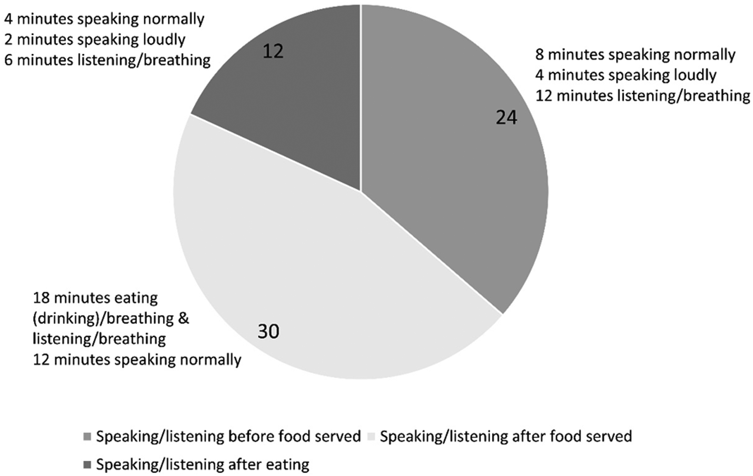
Expiratory means/exposure time (in minutes) estimations for the Guangzhou restaurant event analysis.

Table 10 provides (a) the resulting probability of infections and (b) the potential number of additional people infected, given the net probability of infection. The probability of infection for the three different expiratory means/exposure times is listed as well as the resulting net probability (the chance that at least one of these three conditions occurs). The number of additional people infected is the net probability of infection multiplied by 88 uninfected individuals (for scenario 1) and 20 uninfected individuals (for scenario 2).

Table 10.

Probability of infections and resulting additional patrons potentially infected.

Scenario	Scenario 1 – Whole restaurant		Scenario 2 – Airflow zone of infection
Ventilation	142 cfm (242 m3/h)	196 cfm (333 m3/h)	18.6 cfm (31.7 m3/h)	25.6 cfm (43.5 m3/h)
MERV filter level	4	4	4	4
Virus shedding level	High	High	High	High
Probability of infection – speaking loudly	6.0%	5.4%	26.4%	25.0%
Probability of infection – speaking	2.9%	2.7%	13.7%	13.0%
Probability of infection – breathing	1.2%	1.1%	5.9%	5.6%
Net probability of infection	9.8%	9.0%	40.2%	38.4%
Number of additional infected	9	8	8	8
Normalized error: 9 more infected	–0.4%	–1.3%	–4.8%	–6.6%

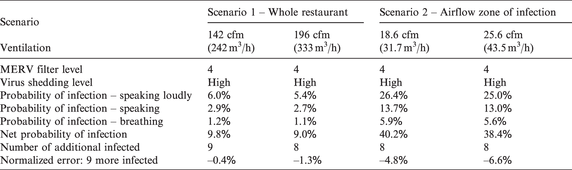
If the estimations are generally correct, then for scenario 1 the model’s normalized error output ranges from –1.3% to –0.4%, underestimating the number of resulting people infected by one or accurately estimating it, depending on the ventilation rates, given the total number of uninfected patrons present in the room. For scenario 2, the model’s normalized error output ranges from –6.6% to –4.8%, underestimating the number of additional people by one for both ventilation rates, given the total number of uninfected patrons present in this zone. So overall:

Scenario 1: Normalized error range: –1.3% to –0.4%

Scenario 2: Normalized error range: –6.6% to –4.8%.

Interestingly, the model’s estimated number of people potentially infected was close to the actual number of patrons infected for both scenarios. As discussed above, the air circulation created by each fan-coil unit limited the flow of aerosols across airflow zones, contributing to the resulting additional infections only occurring within the single airflow zone with the index case. That would suggest this model, which assumes aerosols are instantaneously, continuously and evenly distributed throughout the space being analysed, should be better aligned with scenario 2 than scenario 1. The probability of infections for scenario 2 should better reflect the actual conditions for that airflow zone than the probability of infections for scenario 1 reflect the actual conditions for the entire space.

If this is the case, the fact that the model’s analysis of scenario 1 produced results closely aligned with the actual range of additional individuals infected is likely a coincidence partially driven by the number of patrons present in this case study. For example, instead of 20 uninfected patrons in scenario 2, assume nine uninfected patrons were actually present. Then the resulting potential number of additional patrons infected would be three at 25.6 cfm (43.5 m³/h) of ventilation. For scenario 1, using 77 uninfected patrons for the whole dining space (11 subtracted from 88), the resulting potential number of additional people infected would be seven at 196 cfm (333 m³/h) of ventilation. In this case, there is a greater difference between the two scenarios, and scenario 2 likely represents the more accurate assessment of the model’s capabilities.

Limitations

There are a number of limitations associated with the model itself, as well as the efforts to validate it. Looking specifically at the model’s major limitations, it estimates the probability of infection from airborne transmission only, excluding other routes of transmission such as fomite and direct contact. In addition, the model assumes that the virus-containing aerosols are evenly distributed throughout the space immediately after leaving an infected individual and that the room is a well-mixed condition, with the resulting probability of infection representing an average across the room or space being analysed. It is therefore most applicable for assessing the risk from far-field virus-containing aerosols; it underestimates the risk from near-field virus-containing aerosols that occur at a greater density than the far-field aerosols.

In addition, the quantum generation rates are estimates for many of the listed activity levels and degree of shedding, particularly relative to SARS-CoV-2. As more research is conducted, these values will need to be updated based on what is learned. In addition, due to conflicting data and opinions in the research relative to varying quantum generation rates between adults and children,^11,12 the model currently assumes the same rate for both children and adults.

While the model provides the ability to account for more than one infected individual, it does not allow the user to vary the expiratory means, activity level, quantum of infection, pulmonary ventilation rate or child vs. adult among the infected individuals. The same is generally true for the susceptible individuals, with a few exceptions focused on age.

The model does allow one to differentiate between children and adults for the susceptible individuals, but this distinction is limited to two categories: those less than 18 years of age and those 18 and over. Further variation relative to such factors as pulmonary ventilation (breathing), vaccination rates, etc. are found within each of these two broad categories that are currently not accounted for.

The model does not currently allow one to modify temperature, and it is optimized for interior temperatures between 68°F and 76°F (20°C and 24.4°C). Applying it to other temperature conditions will decrease the model’s accuracy. Future versions will look at incorporating the ability to modify temperature. Mask selections are also limited to the 13 types listed in Table 5.

It may be necessary to consult with various experts, such as consulting engineers, commissioning agents, TAB consultants and/or manufacturers, to verify the most appropriate values to use for such inputs as ventilation rate, RA rate, filter rating, the portable air cleaner’s CADR rating, RH and the upper room UVGI system’s upper zone average irradiance or fluency value.

In addition to hinging on using the most appropriate value for the upper room UVGI system’s upper zone average irradiance or fluency, the associated upper room UVGI system removal factor calculation is also dependent on the actual room conditions being well mixed. Conditions of stagnation or high ACH will decrease the accuracy of the results. Future versions will look at improving the incorporation of the impacts of air flow. At this point there are no known studies linking the susceptibility parameter (Z) for SARS-CoV-2 to RH. As future research illuminates this relationship, the model will need to be updated accordingly.

Vaccine efficacy relative to preventing COVID-19 is still being assessed and the associated adjusted vaccination factor will need to be updated as our understanding of efficacy improves. Nor does the model account for any immunity generated through previous community infections. In those cases where a large number of such individuals (who are also unvaccinated) may be present within a building population, the results will overestimate the probability of infection to an unknown degree.

Despite these limitations, the authors have found the model quite useful in evaluating the relative impacts that different mitigation strategies included in the model have on reducing the risk of infection from SARS-CoV-2 and influenza via an airborne transmission route.

Turning to the validation exercises, in general there are a limited number of documented real-world events, or even controlled laboratory experiments, available for use to validate the model. For those that do exist, many of the parameters needed for the inputs of the model have not been recorded and are difficult to estimate (if estimating can be done at all). The studies for the two events selected have either verified or estimated most of the necessary inputs for this model and appear to have provided the best opportunity to validate the model using actual events. That being said, each event comes with its own set of limitations discussed below.

Skagit Valley chorale superspreading event limitations

The only estimation made that was not justified by information given in the referenced study ²¹ itself was the 30% input value used for RH. As discussed above, the study did not provide any estimate of the rehearsal hall room’s RH during the event. As the heater had been running immediately prior to the choral practice, the interior humidity was estimated to be lower than 50% and the analysis was run for values of 20% RH, 30% RH and 40% RH. Note that the results do not vary significantly between these three RH percentages.

The expiratory means/exposure time input values were based directly on the information provided in the study and are discussed in detail above. However, the simplification made with respect to treating the phase 2 portion of the practice similar to the phase 1 portion could have some minimal impact on the results. This and the uncertainty regarding RH are the two weakest links in this analysis. The measurements and estimates made for the rehearsal hall room size, choir practice OA and RA, the interior temperature, number of infected individuals, viral shedding level, activity level, number of choral members present and the number of resulting choral members infected are discussed in detail in the referenced study. These estimates have generally been well justified by the authors of this study.

Guangzhou restaurant event limitations

Estimates had to be made for RA, temperature and RH with little justification given by the information in the referenced analyses.^86–88 The justification for RA and RH were provided in detail above. There is little justification available for the assumption that the temperature fell within the range optimized for this model. It, along with assigning exposure times to specific expiratory means discussed below, represent the weakest links relative to justifications.

The expiratory means/exposure time input values were based directly on the information provided in the referenced analyses and are discussed in detail above. However, there was little to go on to assign specific exposure times to each expiratory method, relying primarily on the authors’ own experiences. If actual times varied significantly from what was assumed, it could have a noticeable impact on the results. The measurements and estimates made for the dining room size, ventilation OA, fan-coil unit filter, number of infected individuals, viral shedding level, activity level, number of patrons present and resulting number of patrons infected are discussed in detail in the referenced analyses. These estimates have been well justified by the authors of these analyses.

One of the largest questions posed by running an analysis of the Guangzhou restaurant event relative to the model’s assumptions was whether to focus on the entire third floor dining area or only on the single airflow zone with the index case. The latter was likely a closer approximation to a well-mixed environment than the former, and the results of the analysis appeared to support the notion that model applications suffer if the actual environment deviates significantly from well-mixed conditions.

While there are limitations relative to the certainty of some of the inputs for these two events, in the authors’ opinions, they nevertheless validate the generally applicability of the model if its major assumptions are closely met. However, there are several other aspects of the model that still require testing if appropriate documented real-world events or controlled laboratory experiments are found. These include validating the model’s treatment of portable air cleaners, upper room UVGI systems, mask wearing, vaccination, children and the quanta estimates for influenza.

Conclusion

At the beginning of the pandemic in early 2020, there was an expressed need from various building owners, facility managers, occupants and AEC industry consultants to help evaluate the relative contribution of different interior COVID-19 risk mitigation strategies. There was a lack of easily accessible tools and other resources for comparing and ranking different solutions (e.g. increased ventilation, filtration, mask wearing, de-densifying, UV technologies, etc.) for a given context based on both removal efficiency and the probability of infection. This web application ¹ and its underlying model were developed specifically to contextually compare and rank available influenza and SARS-CoV-2 mitigation strategies for making our built environments safer.

In this paper, the authors have provided a detailed overview of the underlying model’s removal and inactivation mechanisms and its specific model of infection, including required inputs, associated assumptions and their justifications as well as the associated limitations. The model was also validated against two documented spreading events to assess its effectiveness, with the normalized errors for both analyses as follows:

Skagit Valley chorale normalized error range for all ventilation rates: –18.4% to +9.7%

Skagit Valley chorale normalized error range for 334 cfm (567 m³/h) OA: –6.9% to –1.3%

Guangzhou restaurant normalized error range for scenario 2: –6.6% to –4.8%

For conditions that generally meet the constraints of the model, these two analyses suggest that the error between modelled and actual number of additional people infected, normalized by the number of uninfected people present, will range from roughly –18.4% to +9.7%. The more certain one can be regarding the input parameters (such as ventilation rates), the smaller these normalized errors will likely be, potentially under 2% as indicated in looking at the range above for the most likely Skagit Valley ventilation rate of 334 cfm (567 m³/h). In addition, the farther actual conditions vary from a box configuration, from an instantaneous, continuous, and even distribution of aerosols, and/or from a temperature range of 68°F–76°F (20°C–24.4°C), the less applicable this model will be to analysing those conditions.

This suggests the model is appropriate to use when its limitations are adequately accounted for and input parameters can be accurately determined. Design team members, commissioning agents, building owners or facility managers attempting to use this tool to assess existing buildings or new designs have a much larger potential to accurately verify input parameters compared to modelling past events, some of which occurred in other countries. The results of such analyses are then more likely to have less errors than the results presented here.

However, additional validation of the Facility Infection Risk Estimator™ ¹ and its underlying model against events including other parameters would be useful. Events involving children or children and adults, varying degrees of mask wearing, activity levels other than light, portable filter units, upper room UVGI systems and influenza instead of SARS-CoV-2 would provide further useful validation. In addition to looking for other events to analyse, the model could also be validated against the monitored effectiveness of mitigation strategies that have been implemented. Opportunities for further development of the model include parameters for SARS-CoV-2 variants, updated data on COVID-19 vaccinations, updated research on masks, updated research on SARS-CoV-2 quanta generation rates, as well as similar updated data/research on influenza.