Sage Journals: Discover world-class research

Abstract

The risk of long range, herein ‘airborne', infection needs to be better understood and is especially urgent during the COVID-19 pandemic. We present a method to determine the relative risk of airborne transmission that can be readily deployed with either modelled or monitored CO₂ data and occupancy levels within an indoor space. For spaces regularly, or consistently, occupied by the same group of people, e.g. an open-plan office or a school classroom, we establish protocols to assess the absolute risk of airborne infection of this regular attendance at work or school. We present a methodology to easily calculate the expected number of secondary infections arising from a regular attendee becoming infectious and remaining pre/asymptomatic within these spaces. We demonstrate our model by calculating risks for both a modelled open-plan office and by using monitored data recorded within a small naturally ventilated office. In addition, by inferring ventilation rates from monitored CO₂, we show that estimates of airborne infection can be accurately reconstructed, thereby offering scope for more informed retrospective modelling should outbreaks occur in spaces where CO₂ is monitored. Well-ventilated spaces appear unlikely to contribute significantly to airborne infection. However, even moderate changes to the conditions within the office, or new variants of the disease, typically result in more troubling predictions.

Keywords

Infection modelling Airborne infection risk COVID-19 Coronavirus SAR-CoV-2

Introduction

The coronavirus disease COVID-19, which causes respiratory symptoms, was declared a pandemic by the World Health Organization (WHO) on the 11 March 2020 – thereby marking its global impact. Transmission of such respiratory infections occurs via virus-laden particles (in this case the virus SARS-CoV-2) formed in the respiratory tract of an infected person and spread to other humans, primarily, via three routes: the droplet (or spray) route, the contact (or touch) route and the airborne (or aerosol) route (e.g. see literature^1–3) According to the WHO, ‘Airborne transmission is defined as the spread of an infectious agent caused by the dissemination of droplet nuclei (aerosols) that remain infectious when suspended in air over long distances and time’.⁴ After some initial resistance, and significant pressure from the scientific community (e.g. see literature^5,6) the WHO finally acknowledged the possibility of airborne infection for COVID-19 on the 8 July 2020.⁷ In the latter part of 2020, multiple mutations to the SAR-CoV-2 virus conspired to give rise to a new variant, named B1.1.7 (see, for example,⁸ for a more detailed discussion). This variant, known also as the Alpha variant, is thought to be significantly more infectious than pre-existing strains⁹ and has been prevalent within the UK and other parts of Europe during 2021. As we look beyond 2021, with new more infectious variants arising (for example, the Delta variant), COVID-19 infection levels remain worryingly high around much of the world. In this article, we focus on assessing the risk of infection of respiratory diseases via the airborne route, taking COVID-19 as an example and, ultimately, deriving a methodology for calculating the expected number of secondary infections that might arise within any indoor space that is regularly attended by the same group of people, applicable to any airborne disease (with estimates for the duration over which infectors remain pre/asymptomatic). We comment on the airborne infection risk for COVID-19 within open-plan offices under a variety of environmental conditions, we include consideration of the Alpha variant B1.1.7 as an illustrative example, and we comment on our findings in the context of the latest variants in our conclusions.

The pioneering work of Wells¹⁰ and that which followed by Riley et al.¹¹ established methods, commonly referred to as the Wells-Riley model, for quantifying the risk of airborne infection of respiratory diseases. Unlike dose-response models, which assess the likely infection response to some (frequently cumulative) dose, Wells-Riley models typically report the complementary probability that no-one becomes infected. As such, these models do not rely on assessing the cumulative exposure which could prove problematic when assessing the infection risk over durations of varied occupancy. Early formulations¹¹ were restricted to indoor spaces which were in a steady-state with a known constant rate of ventilation of outdoor air. The requirement of steady-state is avoided here by the formulation of the model presented by Gammaitoni and Nucci.¹² Rudnick and Milton¹³ further extended the practical application of the Wells-Riley model by negating the need to directly assess nor assume the rate of ventilation of outdoor air. Rudnick and Milton achieved this via the realisation that the risk of airborne infection could be directly inferred via measurements of CO₂ ‘if the airspace is well mixed’. We follow Vouriot et al.^NewRefX in generalising the model of Rudnick and Milton to relax the assumption of a well-mixed space and to further account for variable occupation profiles, ultimately we present a model which allows for quanta generation rates and activity levels which vary in time. The recent work of Peng and Jimenez¹⁴ highlights the ability to account for the expected differences between measurements of a gaseous scalar, e.g. CO₂ and virus particles; namely, particle deposition, viral decay and, potentially, active filtration. Herein, we do not to account for these factors and in this regard, our results represent a conservatively high estimate of the risk.

For many airborne infections, the likelihood of spread within the vast majority of indoor spaces, even over periods of a few hours, is reasonably low (as we show for the coronavirus SARS-CoV-2 and the resulting disease COVID-19). However, there are a significant proportion of indoor spaces which are, for the majority of each working day, attended by the same/similar group of people (e.g. open-plan offices and school classrooms), herein ‘regularly attend spaces’. Our model enables the likelihood of the spread of infection via the airborne route to be calculated (from either easily obtainable monitored data or modelled data) over multiple day-long durations. Hence, in the case of COVID-19 (for which infectors are estimated to remain pre-asymptomatic for 5–7 days), our model calculates the likely number of people that become infected during a period in which a pre-/asymptomatic infector regularly attends the space.

We derive an extended airborne risk model, assess the risk of infection in a modelled open-plan office and use monitored data from a naturally ventilated office to estimate the infection risk. We describe retrospective modelling of an office and then discuss the implications of our findings and draw our conclusions.

The Wells-Riley approach to airborne infection risk

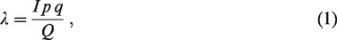
The pioneering work of Riley et al.¹¹ defined the infectivity rate as

λ = \frac{I p q}{Q},

(1)

where I is the number of infected people, p is the breathing (pulmonary ventilation) rate, Q is the ventilation (outdoor air supply) rate and q is the unit of infection, quantum (see literature¹¹ for discussion), which varies significantly between disease, with activity level, and (as with all biologically derived parameters) with individual human beings. For many diseases and relevant activity levels, appropriate values of q have been determined and are reported in the literature.^15–17 – however, significant uncertainties are associated with these values. Moreover, the variability due to individuality is challenging to reflect, as we return to discuss later. In particular, high values of risk are obtained from quanta generation rates derived from so-called ‘superspreading events’¹⁷ – we choose not to focus on such cases but note that should we have done so then the risks reported herein would be dramatically increased (see, for example, Table 1). For a given demographic and activity level within the space, the breathing rate p can be taken as constant and values are widely reported in the literature; the number of infected people I is an input to the model usually taken to be constant.

Table 1.

The expected number of secondary airborne infections, S_I, for COVID-19 arising within an open-plan office (floor plan of 400 m² and floor-to-ceiling height of 3.5 m) occupied by 40 people for 8 h each day over the period that a pre/asymptomatic person remains attending work.

Secondary infections, S_I	Q_pp = 4 l/s/p	Q_pp = 10l/s/p	Q_pp = 20 l/s/p
q = 0.3 quanta/h	0.25	0.13	0.07
Variant B1.1.7	[0.43]	[0.22]	[0.12]
q = 1.0 quanta/h	0.84	0.42	0.24
Variant B1.1.7	[1.4]	[0.72]	[0.40]
q = 5.0 quanta/h	4.0	2.1	1.2
Variant B1.1.7	[6.6]	[3.5]	[2.0]
q = 20 quanta/h	14	7.6	4.4
Variant B1.1.7	[20]	[12]	[7.3]
q = 100 quanta/h	35	26	18
Variant B1.1.7	[38]	[33]	[25]

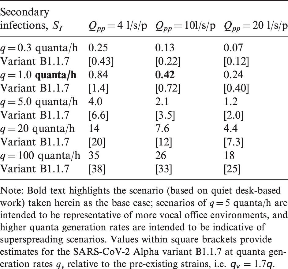
Note: Bold text highlights the scenario (based on quiet desk-based work) taken herein as the base case; scenarios of q = 5 quanta/h are intended to be representative of more vocal office environments, and higher quanta generation rates are intended to be indicative of superspreading scenarios. Values within square brackets provide estimates for the SARS-CoV-2 Alpha variant B1.1.7 at quanta generation rates q_v relative to the pre-existing strains, i.e. $q_{v} = 1.7 q$ .

Riley et al.¹¹ were no doubt aware of the significant challenges in measuring, or even inferring, the outdoor air supply rate to a given indoor space (see Appendix 1 for a detailed discussion). Instead, it was chosen to report the model in a form that can only be applied to indoor spaces for which the air is relatively well mixed and the flows are in steady-state. Under these restrictive assumptions, the classical Wells-Riley equation is recovered, namely that the likelihood, P, that infection spreads within a given indoor space during a time interval T is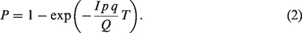

P = 1 - \exp (- \frac{I p q}{Q} T) .

(2)

A model for airborne infection risk in transient spaces with variable occupancy and activity levels

We present a simple model to estimate airborne infection risk which is capable of both exploiting data of the environmental conditions concerning the ventilation (i.e. CO₂ measurements) and accounting for occupancy levels that vary in time. As the insightful work of Rudnick and Milton¹³ highlighted, airborne infection can only occur through the breathing of rebreathed air that is infected. It is important to note that respiratory activity, e.g. breathing, results in a complex multi-phase flow being exhaled. Relative to inhaled air, exhaled air is typically warmer, of higher moisture content (both in the form of vapours and droplets), richer in CO₂ and contains more bioaerosols of which some may be viral particles. The fate of viral particles is of particular relevance to estimating infection risk and determines via which of the three routes (droplet, contact or airborne) infection might occur.^2,3 Those virus particles held in larger droplets may either be directly sprayed onto another individual (risking transmission via the droplet route) or fall to surfaces (potentially giving rise to transmission via the contact route). Following the WHO definition,⁴ virus particles that might give rise to transmission via the airborne route must remain ‘suspended in air over long distances and time’. Therefore, the viral aerosols that can give rise to airborne infection (transmission via the airborne route) will be largely carried with the gaseous emissions exhaled. Directly detecting the presence of viral aerosols within air is challenging, costly and impractical to implement at scale. However, gaseous emissions exhaled by persons are relatively rich in CO₂, and CO₂ sensors of suitable accuracy (say ±50 ppm) are easily obtained for a moderate cost. Hence, monitoring CO₂ as a proxy for air that has the potential to be carrying viral aerosols, while being far from a perfect tracer, has not only legitimate scientific grounds but is also practical to implement at scale.

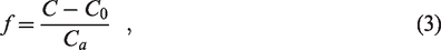
Within most indoor spaces, human breathing is the dominant source CO₂ and so the fraction f of rebreathed air can be inferred from the ratio of the CO₂ concentration within the space (above outdoor levels which we denote C₀) to the concentration of CO₂ added to exhaled breath during breathing, C_a, giving equation (3);¹³

f = \frac{C - C_{0}}{C_{a}},

(3)

where C is the measured CO₂ within the space. Denoting the number of people n within the space and taking the occupancy to be constant gives the fraction of rebreathed air that is infected as

f I / n

. Note that estimating the likelihood of airborne infection via monitored CO₂, from which the fraction of infected rebreathed air is estimated¹³ , makes no stronger assumptions than are already implicit within the classical formulation of the Wells-Riley equation (2). Within the Wells-Riley equation the ratio,

(I p) / Q

is the fraction of infected air estimated to be within the space, while the formulation of Rudnick and Milton¹³ expresses it as

(f I) / n

. In both formulations, the estimate of the fraction of infected air is translated into a likelihood of infection rate via the quanta generation rate. The quanta generation rates utilised in most studies (including the present study) are deduced from data concerning actual far-field infection events. Obviously, these infection events occur as a result of the full physics governing the complex transport of viral particles. As such, the empirical data (underlying the estimates of quanta generation rates) implicitly accounts for some of the differing physics expected to arise between the transport of hypothesised gaseous infectious air (required by Wells-Riley based models) and the actual transport of infectious particles – which for airborne infection to occur must (by the definition of the transmission route) be able to be ‘suspended in air over long distances and time’.

Rudnick and Milton¹³ chose to express their result as equation (4).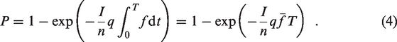

P = 1 - \exp (- \frac{I}{n} q \int_{0}^{T} f d t) = 1 - \exp (- \frac{I}{n} q \bar{f} T) .

(4)

As they point out, this result ‘has very general applicability; it is valid for both steady-state and non-steady-state conditions and when the outdoor air supply rate varies with time’. Furthermore, we highlight that their assumption of a well-mixed space is unnecessary. The fraction of rebreathed air, f, is based on a point measurement of CO₂ which, assuming human respiration is the dominant source of CO₂ (entirely reasonable in the absence of other sources, e.g. unvented combustion), provides, at any instant, a good estimate of the fraction of air at that point within the space that has already been breathed by another individual. This point measurement can be integrated according to equation (4) to give the likelihood that a person (at a location for which the CO₂ sensor within the space is representative of the local environment) becomes infected assuming only that the infected air is relatively well mixed within the uninfected rebreathed air, i.e. it does not require that all the air within the space is well mixed. This implies that, where multiple CO₂ sensors within a single indoor space (inevitably) give different readings, airborne infection risk can be assessed without violation of the modelling assumption being implied; in fact, the different readings within the space could be exploited to obtain estimates of the spatial variation in risk.

We wish to extend the generality of equation (4) with greater applicability in mind, in particular to account for occupancy levels that vary in time. The likelihood that airborne infection occurs within a given space can be determined from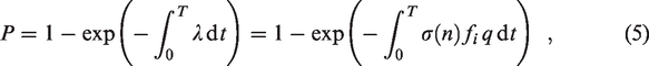

P = 1 - \exp (- \int_{0}^{T} λ d t) = 1 - \exp (- \int_{0}^{T} σ (n) f_{i} q d t),

(5)

with, in the general case, the fraction of infected air f_i within the space being determined by solution of equation (6);

\frac{d f_{i}}{d t} = \frac{I p}{V} - \frac{f_{i} Q}{V},

(6)

where V is the volume of the indoor space which is typically easily estimated, and

σ (n)

is determined based on whether the space is occupied or unoccupied:

σ (n) = 1

for n > 0 and

σ (0) = 0

. For a derivation of equation (5) from first principles see Appendix 1. With suitable selection of the time at which to initiate investigation, the initial condition

f_{i} (0) = 0

will frequently be suitable; typically, values for the breathing (pulmonary ventilation) rate p can be sourced from the literature, and from monitored CO₂ and occupancy levels, the ventilation rate Q can be estimated from equation (18), although as discussed in Appendix 1 such estimates are subject to considerable noise. In spite of this noise, when CO₂ is monitored and occupancy levels are available, then the solution of equation (5) is only lacking knowledge of the time series of the number of infectors I within the space. Note that solution of the full system of equations, e.g. equations (18), (5) and (6), does require the assumption that the air within the space be approximated as well mixed because one is required to calculate the ventilation rates explicitly, unlike simpler models e.g. equations (4) and (7) which do not. Where retrospective modelling is being undertaken to assess a particular outbreak, or spreading event, estimates of these data may be available and attempts to apply the above might prove useful and we turn our attention to informing these cases in our result section. However, with a focus on predictive modelling which, by definition, requires some assumption regarding the presence of infectors I(t), we now consider some appropriate assumptions.

We will either assume that occupants arrive and leave over realistic periods of time (i.e. we model them to not all arrive and leave at once), or our monitored data show this to be so, and thus there exists at least two reasonable principles by which to establish the presence of infectors, I(t). At one extreme, we assume that the infector is always the first to arrive and the last to leave. Alternatively, one could assume that there is always a constant proportion of the (current) occupants infected such that when the space is occupied to design capacity, there is a single infector (this results in the number of infectors, I, taking non-integer values outside full design occupancy which is inconsequential). Should one choose to assume the former, there is a potential that risks are over estimated for scenarios in which occupancy is decreased, or equivalently by allowing more occupants one could under report the risk of the space since a lesser proportion of occupants are infected – in the absence of knowledge as to who is infected, this cannot be reasonable for a comparison of risk with different occupancy levels. As such, we choose to make the latter assumption, i.e. there is always a constant proportion, α, of the (current) occupants infected, i.e. 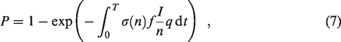$I (t) = α n (t)$ . Doing so renders $I (t) / n (t) = α$ as constant or, alternatively, that the proportion α of the rebreathed air that is infected remains constant, and as such, we can write the likelihood of airborne infection in a far simpler form that still allows for variable occupancy, as equation (7);

P = 1 - \exp (- \int_{0}^{T} σ (n) f \frac{I}{n} q d t),

(7)

where we choose to include presentation with the fraction I/n within the integral to emphasise that both the numerator and the denominator vary in time. Making the assumption that result in equation (7) being valid not only seems reasonable for predictive modelling but it enables the work of Rudnick and Milton¹³ to be extended to predict the airborne infection risk, based on either modelled or monitored CO₂ data, within indoor spaces that also have variable occupancy levels, crucially, without the need to solve the more general equation (5). To solve equation (5) generally, one is required to solve equation (18) to estimate the volume flux as an input to then enable solution of equation (6); doing so requires monitored occupancy levels, CO₂ levels, and relies on the (temporal) gradients in monitored CO₂ levels. Presented in the form of equation (7) and noting

I (t) / n (t) = α

, highlights that precise occupancy levels are not required for the assessment of infection risk, only knowledge of the occupied periods is required.

Throughout this study, we choose to set α such that there is a single infector present, i.e. I(t) = 1, when the space is occupied to design capacity, N_d, which gives $α = I (t) / n (t) = 1 / N_{d}$ . Doing so is as reasonable choice as any other but we note that should comparison of airborne infection risk between separate indoor spaces of differing design capacity be desired then alternative choices should be made. The applicability of the choices to enable predictive modelling via equation (7) will be highlighted throughout our results section, and we then further solve the equations in more general form.

Quantifying the relative risk for changes in environmental management

To examine the effects of a particular change in conditions within a given indoor space, e.g. change in ventilation rate, occupancy level/behaviour, etc., it is informative to define a ‘base case’ scenario for which the likelihood of infection during a time interval T is P₀ and quantify the airborne infection risk of chosen scenarios relative to the base case. We can then define the risk of some test scenario relative to the base case as $R R = P / P_{0}$ , denoting this relative risk as RR_A when a pre/asymptomatic is investigated, i.e. T = T_A. It is worth noting that the relative risk can be written as a ratio of Taylor series expansion of the exponential terms. Doing so can aid approximation since, when the integral $\int_{0}^{T_{s}} σ f \frac{I}{n} q d t$ , is small, the leading order terms in the expansion dominate and the relative risk ceases to be dependent on the quanta generation rate – a notoriously difficult quantity to parameterise which also varies widely between diseases. Hence, for airborne infection risk assessment, the leading order expansion for the relative risk can be reported as valid for all diseases (note that the duration T for which the approximation remains valid does change with disease). Moreover, for any given disease results for the relative risk can be reported with a greater degree of certainty, irrespective of the duration.

Defining absolute risk and the expected number of secondary infections for a given indoor space

An indoor space can be considered as contributing to the spread of a disease if an infected person attends the space for a duration over which it is more likely than not that they infect others. In the case that someone is showing symptoms of the disease, it is reasonable to assume that they cease attending the space or that they be required to do so. Individuals can remain infectious and asymptomatic/presymptomatic for time periods of multiple days (which we denote as T_A) and this renders equation (4) unsuitable for quantifying this likelihood for most indoor spaces. However, for regularly attended spaces, e.g. open-plan offices and school classrooms, the probability P_A that someone becomes infected via the airborne transmission route (assuming an infected person attends the space) can be robustly determined via our formulation equation (7). To do so, time series data for the rebreathed air fraction (monitored or modelled), the occupancy level and quanta generation rate are required over the duration T_A. For a given disease, assuming the activity levels (per capita) remain broadly the same within the space, the quanta generation rate can be assumed constant. For real-world assessment, f and n can be obtained from monitored CO₂ and occupancy data, respectively. Moreover, for model cases, this can easily be calculated. We demonstrate examples of this for model building spaces, and using monitored data from an existing open-plan office taking COVID-19 as a case study.

As pointed out by Rudnick and Milton,¹³ their formulation equation (4) can be used to determine what they term a ‘basic reproductive number’ for an airborne infectious disease within an indoor space. Herein, we describe this as the expected number of secondary infections , S_I, via the airborne route that arise within an indoor space when an infectious individual is attending the space and everyone else is susceptible. For regularly attended spaces, this is simply calculated from the probability of someone becoming infected over the pre/asymptomatic period multiplied by the number of susceptible people, giving equation (8);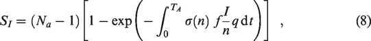

S_{I} = (N_{a} - 1) [1 - \exp (- \int_{0}^{T_{A}} σ (n) f \frac{I}{n} q d t)],

(8)

where N_a is the total number of people that regularly attend the space. We earlier pointed out, calculations of the likelihood of infection via either equation (4) or via equation (7) do not require the assumption that all the air within the indoor space is well mixed. However, for the expected number of secondary infections to be a meaningful estimate, then equation (8) requires that the likelihood of infection to be representative of the risk throughout the occupied indoor space. If all the air within the space is well mixed, then this is simply satisfied; otherwise, multiple CO₂ measurements should be taken, within the breathing zone, to assess the degree of spatial variation.

To summarise our modelling, we have developed practical statistics to assess airborne infection via relative risk-based scenario testing (RR), the absolute probability of infection (P_A) and the expected number of secondary infections for an indoor space (S_I). All of these can be calculated by obtaining/modelling representative CO₂ data. Moreover, for measured/modelled CO₂ distributions within the space, on assuming the infected and uninfected rebreathed air are well mixed, these statistics can be calculated and their variation within the space investigated.

Determining appropriate quanta generation rates

As with all Wells-Riley based infection modelling, an input parameter for which great uncertainty abounds is the quanta generation rate, q – with the novelty of COVID-19, this uncertainty in compounded. Given the uncertainty, we include results of scenario tests at various feasible levels of q, which span nearly four orders of magnitude. All of our choices regarding quanta generation rates stem from the data presented in the study of Buonanno et al.¹⁸ As a base case, which we deem appropriate for the regularly attended spaces on which we focus (namely, open-plan offices and class rooms), we take a value of q = 1 quanta/h – this is obtained by taking $c_{x} = c_{i} c_{v} \approx 7 \times 10^{6}$ RNA/ml, where $c_{i} = {0.1, 0.01}$ is the ratio between infectious quantum and the infectious dose expressed in viral RNA copies, and $c_{v} = {7 \times 10^{7}, 7 \times 10^{8}}$ RNA/ml is the viral load measured in sputum. These values obtained by consideration that, for most of the time in most open-plan offices and classrooms, most of the occupants are sitting breathing with perhaps a small number vocalising – the data for whispered counting fall between these two activities and is more close to breathing – as such, for our base case, we take data for whispered counting from Buonanno et al.¹⁸ and use their results to map our selected values of c_x to values of quanta generation rates q. Moreover, we consider a scenario in which the occupants within the open-plan office or classroom are (on average) all vocalising/talking (e.g. a call-centre or noisy classroom), taking again $c_{x} \approx 7 \times 10^{6}$ RNA/ml gives $q \approx 5$ quanta/h. In addition, we consider a scenario in which the viral load in sputum is somewhat reduced, i.e. $c_{v} \approx {2 \times 10^{7}, 2 \times 10^{8}}$ RNA/ml, giving $q \approx 0.3$ quanta/h.

Mutations of the SARS-CoV-2 virus have given rise to new variants of the disease, the first of these to really take hold was named B.1.1.7 and now termed the Alpha variant. The Alpha variant was widely detected in certain geographical regions (within the UK in particular) in the latter part of 2020 (see Kupferschmidt⁸ for details and we choose to include analysis of the this variant due to the data being currently available. This variant, which spread quickly across international borders, is believed to be potentially around 70% more transmissible than the ‘pre-existing’ strains of the virus.^9,19 It is, as yet, unclear by which mechanisms the transmission of the new variant is increased; however, it is an important development which demands analysis. We therefore include estimates for the airborne infection of variant B1.1.7 within our results. To do so, we assume that the increase in transmission of B1.1.7 via the airborne route might be proportional to the total increase and, for the various scenarios considered, take quanta generation rates for the variant, q_v, to be 70% higher than those corresponding to pre-existing strains of the virus, i.e. $q_{v} = 1.7 q$ .

Predictive modelling of airborne infection using COVID-19 as an example

Application to a model open-plan office

By way of example, we first consider a moderately sized open-plan office, of floor area 400 m² and (a generous) floor-to-ceiling height 3.5 m, which is designed to be occupied by 40 people.²⁰ We assume that occupants arrive steadily between 08:00 and 09:00 each morning, each take a 1 h lunch break during which they leave the office, and leave steadily between 17:00 and 18:00 each day. While within the office we assume that (on average) each occupant breathes at a rate of approximately p = 8 l/min with a CO₂ production rate of 0.3 l/min, giving $C_{a} = 0.038$ and we take the outdoor CO₂ level to be 400 ppm.¹³ As a base case, we assume ventilation provision in line with UK guidance for office spaces, i.e. a ventilation rate per person of Q_pp = 10 l/s/p,²⁰ or a total ventilation rate of Q = 400 l/s.

Our model run for this open-plan office gives, for the base case, the absolute risk of infection during a period of pre/asymptomatic COVID-19 infection as $P_{A} = 1.1 %$ . If one had have taken the classical Wells-Riley model (2), taking there to always be a single infector present and T to be the simple sum of occupied hours (i.e. T = 40 h), the level of risk reported would have been $P = 1.3 %$ , around 20% higher. We note that the key benefit of our model is the ability to use monitored CO₂ and occupancy data as we demonstrate.

The impact of varied quanta generation rates

We first examine the impact of varied quanta generation levels; namely, $q = {1, 0.3, 5}$ on the likelihood of airborne infection. Figure 1 plots the absolute likelihood that someone becomes infected within the office via the airborne route over the period during which an infector is expected to remain pre/asymptomatic, i.e. five working days (since the period of pre/asymptomatic infectivity for COVID-19 is estimated as five to seven days). The plot shows that in the base case, the absolute risk, P_A, of airborne infection within this open-plan office is around 1.1% (or assuming a lower viral load is appropriate the risk drops to around $P_{A} = 0.3 %$ ). However, if the open-plan office was a call-centre, then this risk that someone becomes infected through attending work increases to above 5%. These results correspond to estimates for the quanta generation rates based on the work of Buonanno et al.¹⁸ on data for ‘pre-existing’ strains of the SARS-CoV-2 virus. In the latter part of 2020, mutations gave rise to a new variant of the virus B1.1.7 which is already prevalent in some geographical regions. Within Figure 1, dashed lines show estimates for the likelihood of airborne infection for the B1.1.7 variant based on the current data which suggest this variant may be 70% more effectively spread. Since for the scenarios being tested, the likelihoods remain relatively linear in response to changes in infectivity, the risks are increased by a factor of around 1.7 in all three scenarios, i.e. for the base case scenario with variant B1.1.7, the airborne infection is predicted to be nearly 2%.

Figure 1.

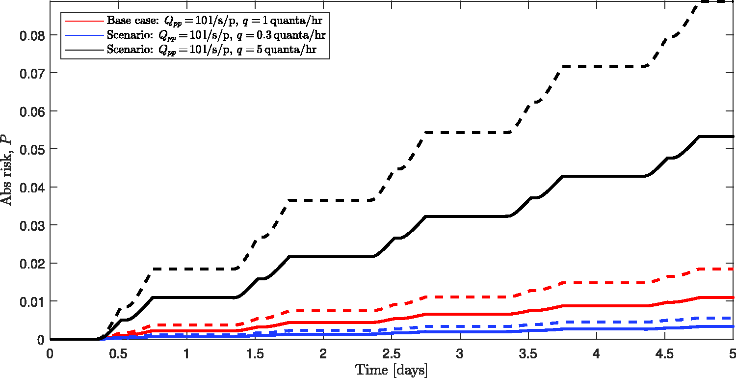
The variation in the likelihood of infection with time over the five-day pre/asymptomatic period with ventilation in line with UK guidance, i.e. Q_pp = 10 l/s/p. Solid curves mark the risk with differing quanta generation rates assumed for the pre-existing SARS-CoV-2 strains: blue denotes q = 0.3 quanta/h, red denotes q = 1 quanta/h and black denotes q = 5 quanta/h. The correspondingly coloured dashed curves mark estimates for the variant B1.1.7 for which we take the quanta generation rates to be $q_{v} = 1.7 q$ .

One can, of course, examine the relative risk of airborne infection; as expected from consideration of Taylor series expansions of the exponential terms, the results are broadly constant in time, with the relative risk taking an initial value of $q / q_{0}$ (or $q_{v} / q_{0}$ ), and then remaining dominated by the ratio of the quanta generation rate between the scenarios and/or variants. For example, in this office at the end of a pre/asymptomatic period, examining the scenario that the open-plan office changes to become equivalent to a call-centre gives the relative risk as $R R_{A} = 4.9$ (for $q / q_{0} = 5$ , and taking $q_{v} = 1.7 q$ gives $R R_{A} = 8.2$ ), and imagining that the appropriate viral load for the disease, for some reason, becomes lower gives $R R_{A} = 0.3$ (for $q / q_{0} = 0.3$ ). One can see that for these cases the relative risk is well predicted by a linear approximation (taking only the first order terms in the Taylor series expansion of the probabilities), i.e. the relative risk is approximately equal to the ratio of quanta generation rates between the scenarios.

The importance of ventilation/outdoor air supply rates

The qualitative increase in the airborne infection risk within the office during a period of pre/asymptomatic infection for varied outdoor air supply rate per person, Q_pp, is broadly similar to that shown in Figure 1. Over the full pre/asymptomatic period, the base case (of course) again gives $P_{A} = 1.1 %$ for pre-existing strains of the SARS-CoV-2 virus. Doubling the ventilation rate per person to Q_pp = 20 l/s/p decreases the likelihood to $P_{A} = 0.6 %$ , and decreasing the outdoor air supply rate per person to Q_pp = 4 l/s/p results in $P_{A} = 2.2 %$ (see Table 1).

Examining the relative risk RR, for scenarios of changing ventilation rates, then RR takes an initial value of unity and only over time does the ventilation alter the accumulation of infected re-breathed air within the space. In this open-plan office, in the case that the ventilation is doubled from one scenario to the next, the relative risk reaches an approximately steady value of $R R \approx 0.55$ around 6 hours after being occupied (see Figure 2), and in the case of decreased ventilation ( $Q_{p p} / Q_{0} = 0.4$ ), then $R R \approx 2.0$ is reached after approximately 10 h. At the start of each working day, as the office is reoccupied, the relative risk can be seen to deviate from, then return back to, its steady-state value (Figure 2), this is as a consequence of transient effects – as the fraction rebreathed air increases at different rates in each scenario (due to the differing ventilation rates). Transient effects that occur at the end of the day do not affect the infection risk since the office is unoccupied. These deviations lessen each day as the transients have a smaller impact on the integral risk; the deviations are also more pronounced in the case that the ventilation is reduced, i.e. the black curve in Figure 2.

Figure 2.

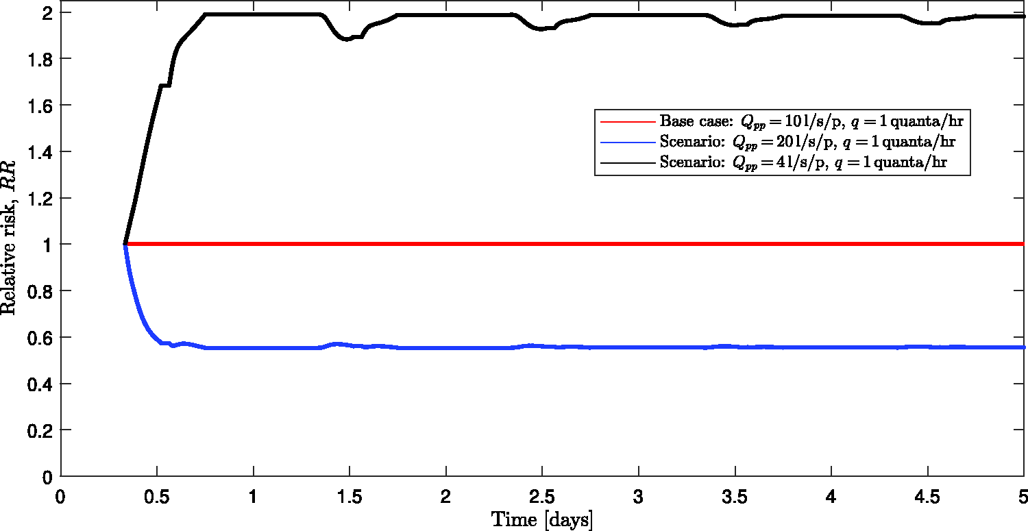
The variation in the relative risk, RR, of infection with time over the five-day pre/asymptomatic period. The different curves highlight different scenarios, namely: the base case, Q_pp = 10 l/s/p (red), increased ventilation rate, Q_pp = 20 l/s/p (blue) and decreased ventilation, Q_pp = 4 l/s/p (black). The periodic deviations from the steady-state values of RR arise due to transient effects as the office is reoccupied each day.

The expected number of secondary infections for an open-plan office

We ran our model for the expected number of secondary airborne infections, equation (8), for a period of pre/asymptomatic infectivity (five to seven days, i.e. spanning five working days) varying both the quanta generation rate (of ‘pre-existing’ virus strains $q = {0.3, 1.0, 5.0}$ quanta/h) and the outdoor air supply rate air supply rate ( $Q_{p p} = {4, 10, 20$ } l/s/p). The results are presented in Table 1 and suggest that, for these environmental conditions with quiet desk-based work being conducted, it is unlikely that an employee’s time within the office will significantly contribute to the spread of COVID-19 via the airborne route. However, if the RNA copies/viral load are as expected by Buonanno et al.,¹⁸ i.e. $q \approx 1$ for quiet desk-based work, but the office is poorly ventilated then the expected number of secondary infections arising within this office may hover dangerously close to unity for pre-existing virus strains; should the B1.1.7 variant become prevalent then a single infection within the office could be expected to give rise to around 1.4 new infections just via the airborne route. Alternatively, if the office is used for particularly vocal activities, e.g. a call-centre or sales office (i.e. making $q \approx 5$ more appropriate for pre-existing strains), then, these spaces may significantly contribute to the spread of COVID-19 via the airborne route even when ventilated in line with current UK guidance – with the situation only worsened in the presence of the B1.1.7 variant.

To end this section, we note that Buonanno et al.¹⁸ report far higher quanta generation rates for ‘superspreaders’. The definition of a superspreader is unclear and far from unanimous. We note that the term may refer to specific combinations of the particular activity being undertaken, the environmental quality, and the biological response of individuals. Within Table 1, we include two sets of scenarios (based on q = 20 quanta/h and q = 100 quanta/h, respectively) which report the expected number of secondary infections that might arise within our office should some superspreading event occur within. The results are worrisome with the majority of employees becoming infected from the presence of a single infector in many of the scenarios examined. We hope that the conditions that might be required to give rise to superspreader events are unlikely to occur over durations comparable to a full pre/asymptomatic periods; if so, these scenarios may prove to be overly pessimistic.

The benefits of reduced occupancy

The above results suggest, under certain conditions, occupation of an open-plan office may contribute to the spread of COVID-19 just by the airborne route. This is troubling as the airborne route is perhaps the most difficult transmission route to mitigate against with appropriate ventilation being the primary mitigation strategy. Employers should help to mitigate the airborne spread of COVID-19 by ensuring ventilation systems are sufficient to comply with guidance and that they are properly maintained. However, large-scale changes to the ventilation provision, for example to double the supply of outdoor air, are costly and will take time to implement appropriately (e.g. ensuring that the heating provision, and other factors, are also adequately adjusted or upgraded). One course of action that may be more immediately appealing is to consider keeping the occupancy reduced. For example, introducing week-in week-out working would result in the occupancy being halved. However, the ventilation system can be set to keep running at the full design capacity (which in our model office was Q = 400 l/s in the base case scenario). Doing so results in the expected number of secondary infections that might arise via the airborne route within our office being reduced by a factor of about four, because, all else being equal, in this example, the probability of an infector being present is roughly halved compounded by the fact that there are half the number of people to infect. This fourfold reduction in secondary airborne infections is significant, while the strategy provides opportunities for employees to attend the office in a manner which might be of practical benefit to themselves and their employer alike. Reducing the occupancy by a factor of r results in the expected number of secondary infections that might arise via the airborne route being reduced by a factor r² for all the scenarios considered herein.

Airborne infection risk from monitored data in open-plan office

To demonstrate the application of our model to indoor spaces with monitored CO₂ and occupancy data, the latter being obtained via analysis of video images of the office space, we were provided access to data recorded by the ‘Managing Air for Green Inner Cities (MAGIC)’ project (http://www.magic-air.uk). The data were recorded in a small office which had a design capacity of eight people, although during the times for which we were provided data never more than six people attended the office. The office is naturally ventilated with openable sash windows on opposite sides of the building. The floor area is approximately 37.6 m² and the floor-to-ceiling height is 2.7 m; Song et al.²¹ provide full details of the monitored space and the monitoring equipment used, but it should be noted the monitored office is not of a modern design and is not well sealed nor well insulated. For monitored data, it is worth considering how to appropriately select the ambient CO₂ concentration, C₀, since atmospheric levels do vary slightly and CO₂ sensors can exhibit a base-line drift over time. For all our analysis based on monitored CO₂ data, we decided to allow the ambient CO₂ concentration to vary taking its value each day to be the mean value observed between 05:00 and 06:00.

The role of opening windows in reducing risk

Figure 3(a) and (b) shows the occupancy profiles during two days in 2017. During 29 September, the windows were opened on both sides of the building (providing an opened area of 0.24 m²) at around 09:00 and remained so until after 20:00, while on 5 October, the windows remained closed all day and we note that the spike in CO₂ at around 16:15 on this day corresponds to a brief visit during which 22 people were in the office. The monitored CO₂ profiles (Figure 3(c) and (d)) were obtained at six locations of differing heights (between 73 cm and 242 cm from the floor) and positions within the office. It is most striking that the CO₂ levels are markedly higher on 5 October when the windows remained closed. Crucially, these elevated CO₂ levels translate into increased risk of airborne infection for the occupants – in this case, the risk of infection being approximately doubled on the day when the windows remained shut. In addition, at times (e.g. between about 14:00 and 17:00 on 25 September), there is a marked variation in measured CO₂ levels dependent on location. It follows that this variation in CO₂ is reflected in the infection risk levels which indicates that the location within the office at which one was breathing affected the risk of infection by around 20% on the day the windows were closed and a much more substantial variation on the day the windows were open. This highlights the need for careful placement of sensing equipment from which data is often obtained only at a single point within a space with inferences being taken as representative for all occupants.

Figure 3.

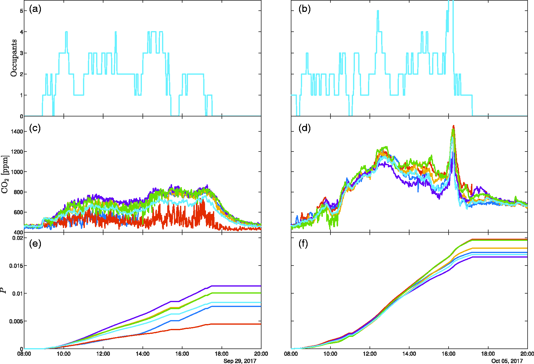
The intra-day variation in occupancy (upper panes, (a) and (b)), monitored CO₂ (middle panes, (c) and (d)) and the corresponding risk of airborne spread of COVID-19 (lower panes, (e) and (f)) during 29 September 2017 (left-hand panes, (a), (c) and (e)) and 5 October 2017 (the right-hand panes, (b), (d) and (f)). Data are plotted from six CO₂ monitors placed at various locations and heights (between 73 cm and 242 cm from the floor). On the 29 September (left-hand panes), windows on opposite sides of the room were opened (creating an opened area of around 0.24 m²) from 08:00 until 20:00, while on the 5 October (right-hand panes), the windows remained closed all day.

Figure 4(a) shows the occupancy data for the monitored office over a five-day period in September 2017. During this five-day period, the office windows were open for some significant portion of each day. The accompanying monitored CO₂ data is shown in Figure 4(b) and it should be noted that data are missing between 13:30 and 19:00 on 27 September. The risk of airborne infection for COVID-19 is shown in the lower pane with the risk rising gradually over the period of pre/asymptomatic infectivity reaching an absolute risk $0.059 \leq P_{A} \leq 0.064$ depending on where within the office the occupant would have been located. We note that two of the sensors were positioned very close to the windows. However, perhaps surprisingly, for the five-day period, the CO₂ concentrations measured in these positions were not significantly below those measured elsewhere within the office, and the airborne infection risk estimated from the sensors near the windows was not systematically lower than those positioned in the centre of the room. One of the sensors placed close to the window, the data marked in reddish-orange in Figures 3(c), (e), 4(b) and (c) does show levels which are significantly below the other sensors during 29 September – however, as Figure 4(c)) shows over the five-day period (25–29 September) the impact is not drastic with the risk inferred from all sensors lying within $\pm 5 %$ of the mean. The expected number of secondary infections for the monitored office over this period is $0.3 \leq S_{I} \leq 0.32$ – reassuringly below unity and indicating that this naturally ventilated office was likely to have been receiving somewhere between 10 l/s/p and 20 l/s/p (see Table 1). From examination of the monitored office during periods when the windows were closed, the expected number of secondary infections might approximately double to $S_{I} \approx 0.6$ . We note, however, that these risks might be considerably higher for more modern well-sealed offices.

Figure 4.

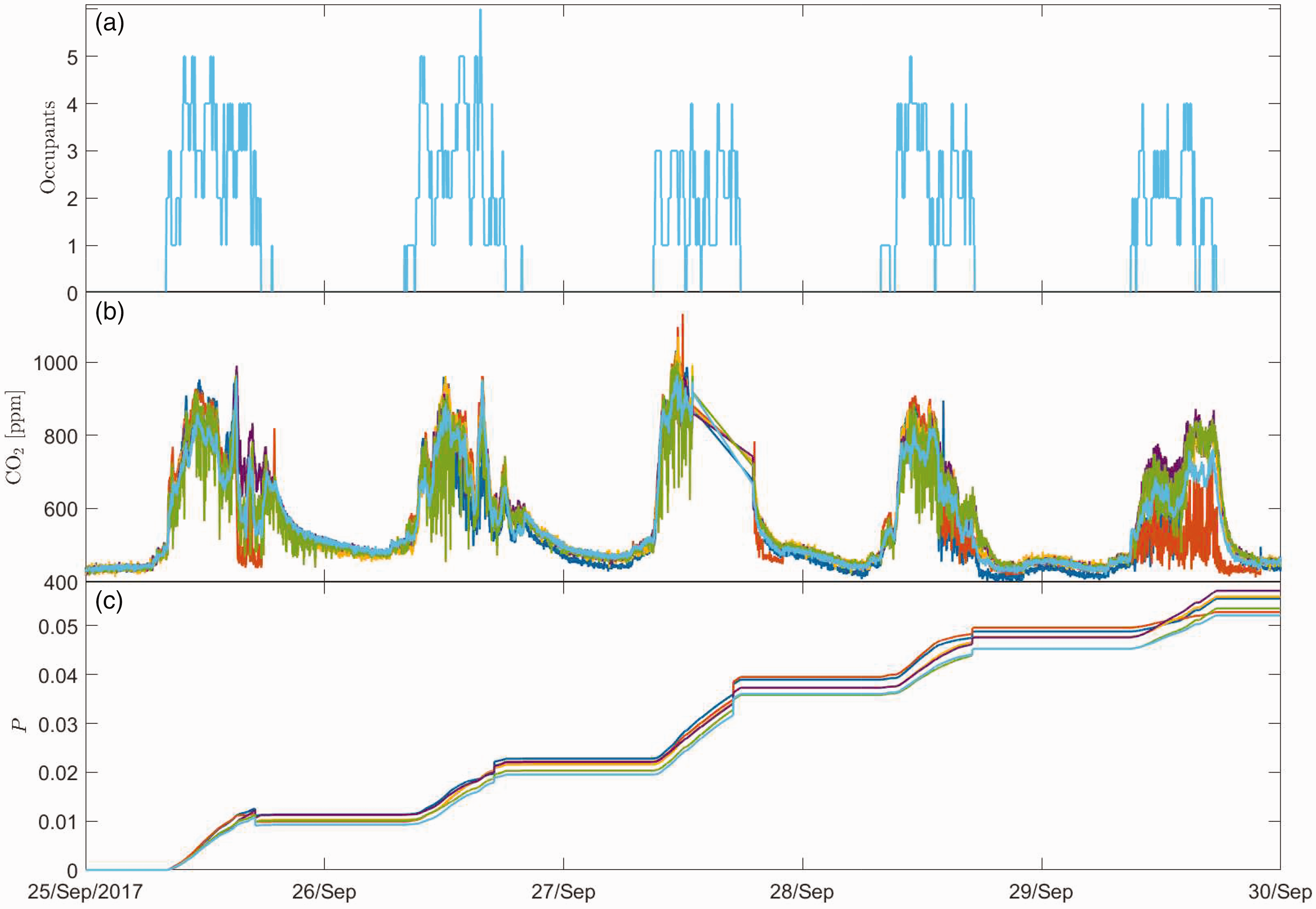
The variation in (a) occupancy, (b) monitored CO₂ and (c) the corresponding risk of airborne spread of COVID-19, over a period of pre/asymptomatic occupancy of the monitored office. Data are plotted from six CO₂ monitors placed at various locations and heights (between 73 cm and 242 cm from the floor).

Retrospective modelling using COVID-19 as an example

In the following section, we chose to examine a full pre/asymptomatic period within an open-plan office. However, the methodology for airborne risk evaluation we present is applicable to any shared indoor space for which, while the number of occupants can vary throughout, the occupant population should only slightly exceed the observed maximum occupancy.

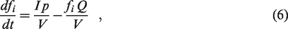
Where retrospective modelling of an outbreak is desired, it is natural to assume that the infector’s occupancy profile may be known (or at least estimated) and so invoking the simplifying assumptions that lead to our predictive model, equation (7), is likely to be inappropriate. In order to account for bespoke infector occupancy profiles, one must return to the general equation for the likelihood of airborne infection, i.e. equation (5), which requires solution of both equation (18), to determine the ventilating flow though the space and equation (6), to determine the amount of infectious airborne material present. This retrospective modelling requires that the ventilation flows are inferred from the monitored CO₂ and that these flows are then utilised to determine the dilution of the airborne infectious material being emitted by any infectors as and when they are present. As such, for this retrospective modelling, it is necessary to assume that all of the air within the space is well mixed. Where indoor concentrations are expected to vary spatially within a single space, then multiple CO₂ monitors can be deployed to establish estimates of the errors introduced by the necessity to assume well-mixed air. The CO₂ data presented herein is one such case, a naturally ventilated office with no mechanical means to generate a well-mixed environment. However, despite having sensors positioned both in the centre of the room and near the windows, over the full five-day period (Figure 4), the spatial variation in CO₂ concentration alone only changes the risk inferred from any sensor by at most $\pm 5 %$ of the mean; this despite the fact that for certain periods CO₂ concentrations varied considerably between the sensors.

To test the methodology of retrospectively inferring the risk from CO₂ measurements, we select the data from only one of the sensors (plotted in green in Figures 3 and 4); we do so to add the clarity of comparison between results of different forms of analysis, the one sensor used was selected because it is relatively typical within the set of six sensors. We note that results reported hereinafter have been tested for each of the six sensors with no notable differences arising. In order to establish the validity of the method, we first compare the results from the retrospective analysis to those of the ‘true’ predicted risk from our previous analysis. Within Figure 5, the result of the risk from the predictive method are plotted as the black curve resulting in $P_{A} = 0.054$ . However, when the same CO₂ data are used to solve equations (18) and (6), which are then substituted into equation (5) and integrated, i.e. the retrospective method (with the proportion of infectors, I/n, taken to be constant solely to enable direct comparison to the predictive method), the airborne infection risk (marked by the red curve) is significantly lower with $P_{A} = 0.044$ . This difference arises because the retrospective methods require discrete observational data to be differentiated which introduces non-trivial errors, even when using a central differencing scheme. These errors can be avoided by fitting the observed data using cubic-spline curves, re-sampling the fitted spline curves at higher a frequency before differentiating and then time integrating to obtain the risk. However, to avoid observable errors in the risk, one needed to re-sample our data, which were recorded every minute, at a frequency increased by a factor of at least 30; this proved computationally intensive even for a week-long data set. As an alternate solution, passing these data through low-pass filters was found to effectively reduce these errors without significant loss of computation performance. For all our data, the airborne infection risk implied by the retrospective method was insensitive to the choice of low-pass filter (we tested the finite-duration impulse response, infinite-duration impulse response (IIR), and a third-order Savitzky-Golay filter in Matlab) and also relatively insensitive to the passband frequencies $T_{f}^{- 1}$ with 20 min $\leq T_{f} \leq 240$ , yielding notionally the same results (similarly in the case of the Savitzky-Golay filter T_f denotes the duration of the filtering window).

Figure 5.

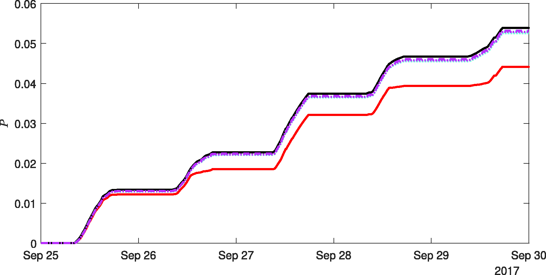
The variation in the likelihood of airborne infection risk, P, over a five-day period based on CO₂ data from one sensor within the monitored office. The black curve shows the likelihood based on the predictive methodology equation (7), i.e. the same data from this sensor are shown in Figure 4. Estimates of the airborne infection risk, taking the same disease parameterisation and occupancy, but reconstructing the risk using the full equations using the raw CO₂ data are marked with by the red curve. Estimates of the airborne infection risk reconstructed using the full equations and CO₂ data subjected to a low-pass filter are marked with by cyan curves for infinite-duration impulse response filter and magenta curves for the Savitzky-Golay filter. Data are shown for passband frequencies, and filtering windows, based on T_f = 20 min (dotted curves) and T_f = 240 min (dashed curves).

Figure 5 also shows the retrospective airborne infection risk inferred from the CO₂ data, with a passband frequency and filtering window set by T_f = 20 min, for an IIR (dotted cyan line) and a Savitzky-Golay filter (dotted magenta line), and with T_f = 240 min for an IIR (dashed cyan line) and a Savitzky-Golay filter (dashed magenta line) – all of which result in $P_{A} = 0.053$ (when rounded to two significant figures). As such, we can report that with appropriate filtering, airborne infection risk can be reconstructed retrospectively based on monitored CO₂ data. Based on all available data, the method appears to provide good accuracy when the CO₂ data are subjected to a low-pass filter, irrespective of the choice of filter and exhibit an adequately low sensitivity to the choice of passband frequency, or filtering window.

For completeness, each night the CO₂ concentration within the office notionally reached ambient levels and these ambient levels varied slightly from day-to-day, and we observed singularities in the implied flow rate when the denominator of the right-hand term of equation (18), namely $(C - C_{0})$ , became zero. These could have either been avoided by setting the ambient CO₂ concentration artificially low but that would result in artificially high risk being reported. Instead, we replaced the denominator with $max (C - C_{0}, 10^{- 5})$ which both avoided the singularities and did not overstate the risk – this insertion can be justified upon realising that the tolerance of CO₂ monitors typically far exceeds $10^{- 5}$ or 10 ppm. It is interesting to note that irrespective of the filtering, we were never able to obtain estimates of the instantaneous ventilation flow rates, these typically fluctuated unreasonably in the range $\pm 100$ air changes per hour (ACH). However, since these instantaneous ventilation flow rates only affect the likelihood via equation (6) which is then integrated twice with respect to time, such unreasonable fluctuations do not, in practice, significantly affect estimates of airborne infection risk.

In order to demonstrate the flexibility of this method, we could examine the effect on the likelihood of airborne infection of a particular arrival and departure schedule of an infector during the five-day period. However, it is widely accepted that the virulence of a COVID-19 infector might vary substantially during their pre/asymptomatic period and, as such, it is perhaps more relevant to consider such a case. The precise variation in a typical infector’s virulence during the infectious period is not yet well evidenced so to demonstrate the ability to model such data, should it become available, we consider an extreme example where on only one of the pre/asymptomatic days the infector becomes significantly more virulent. We parameterise this temporal variation in infectivity via the quanta generation rate q(t), and for reasonable comparison, we ensure that the integral of q(t) over the five days remains unchanged. Consider the arbitrary case that on day 3, the disease was particularly infectious with q(t) = 3 quanta/h, while selecting $q (t) = 0.5$ quanta/h for the other four days, thus ensuring that an average of q = 1 quanta/h. In order to properly account for varied quanta generation rates, the subject of the integral in equation (5) needs to be evaluated via equation (9).

\frac{d f_{i} q}{d t} = \frac{I p q}{V} - \frac{f_{i} q Q}{V} .

(9)

The results are shown in Figure 6. For reference, the likelihood of airborne infection with constant q = 1 quanta/h is shown for the predictive method, by the black curve, and the retrospective method (based on low-pass filtered CO₂ data), by the dashed magenta curve – both assuming I/n is constant, purely to enable comparison. Two blue curves mark the results for the case of variable infectivity being considered. For one, the more infectious day was taken to be the third day (27 September), and for the other it was taken to be the fourth day (28 September). Both blue curves initially indicate lower risk, for the days on which $q (t) = 0.5$ quanta/h, and then show marked increases in the risk on the more infectious day before continuing to increase (at a rate less than that of the constant quanta generation rate). The risk for the case where the disease was more infectious on 27 September finishes significantly above the risk of the constant quanta generation rate case; the opposite is true for the case where disease was assumed more infectious on 28 September. This is simply because the integral CO₂ levels during 27 September were above the average for the five days and those on the 28 September were below the average. This is in line with expectations based on inspection of the system of equations, since the risk is determined by the integral of $f_{i} q$ over time. Crucially, these results provide successful demonstration of the principles of retrospectively evaluating the airborne infection risk for a general case based on actual CO₂ measurements.

Figure 6.

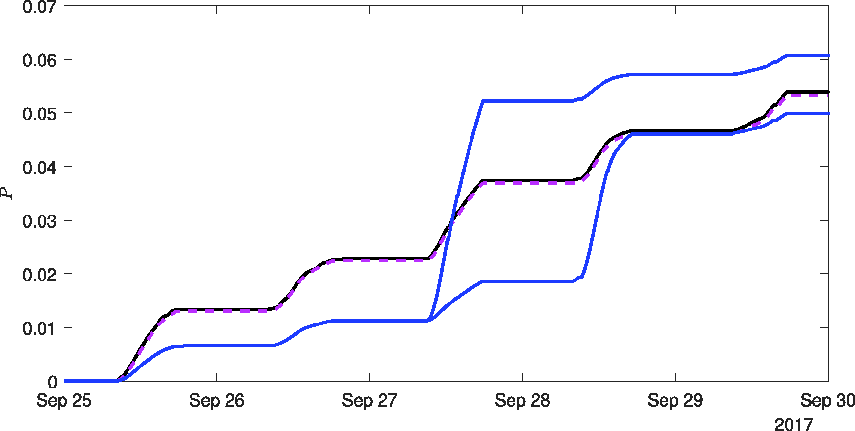
The variation in the likelihood of airborne infection risk, P, over a five-day period based on CO₂ data from one sensor within the monitored office. For constant quanta generation rate of q = 1 quanta/h, the black curve shows the likelihood based on the predictive methodology (7) and the dashed magenta curve the likelihood reconstructed from the low-pass filtered CO₂ data. The blue curves show the results assuming the disease is such that the infectivity on day 3 is greater than on the other four days, but for fair comparison, we parameterise the disease such that integral quanta over the five-day period remains unchanged. In this case, we chose values of q = 0.5 quanta/h for four days, rising to q = 3 quanta/h on the more infectious day. The plot shows the final risk can be either above (when q = 3 quanta/h on the second day, i.e. 27 September) or below (when q = 3 quanta/h on the third day, i.e. 28 September) the results for the constant quanta case, with this being simply determined by whether rebreathed air was more prevalent (than the average over the full duration, here five days) during the more infectious period, or not.

Discussion and conclusions

Taking COVID-19 as an example, relatively simple models have been derived to estimate the likelihood of airborne infection within indoor spaces which can account for variable occupancy levels, bespoke infector behaviours and diseases for which the infectivity varies in time during the infectious period. Our models require only monitored or modelled data for CO₂, occupancy and infector levels and estimates of appropriate quanta generation rates (which in the most general case can vary in time). A modelled office and, separately, monitored data were used to demonstrate results.

We conclude that for open-plan offices, regularly attended by the same/similar people, which have ventilation provision in line with UK guidance,²⁰ then attendance of quiet desk-based work is unlikely to significantly contribute to the spread of COVID-19 via the airborne route. However, this changes should these spaces be poorly ventilated (e.g. l/p/s) since then, through a single infected person attending the office, the expected number of people becoming infected via the airborne route is close to unity, and estimates rise well above for the SARS-CoV-2 variant B1.1.7. (known also as the Alpha variant). Even for adequately ventilated spaces if the occupants are very vocal (e.g. a call-centre) then, in the presence of a single infector, one could expect attendance of the office to give rise to between two and four new COVID-19 infections, and so for these spaces, we conclude that attendance could significantly contribute to the spread of COVID-19 via the airborne route. We note that increasngly infectious variants are now prevalent in many parts of the world, e.g. the Delta variant, our models may be helpful in assessing the expected impact of these and future variants. Due to their ill-defined nature, we choose not to focus on superspreader scenarios but instead we primarily considered conditions more in line with the median of the population. Should we have chosen to examine superspreaders, then our results would have been more alarming.

The above conclusions highlight that by making readily achievable changes to the indoor environment can alter whether, or not, the attendance of work within an open-plan office might significantly contribute to the spread of COVID via the airborne route. These changes include, altering ventilation between rates supplied to working offices, and changes in behaviours that can be expected to occur with different office usage. More successful variants of the virus, e.g. B1.1.7, may only result in a greater number of the environmental scenarios giving rise to significant numbers of secondary infections. This highlights that as, and when, communal workplace practices are re-established, there is a need to better mitigate against the airborne spread of COVID-19 (see, for example, Burridge et al.^NewRefY for a detailed discussion), while maintaining every effort to reduce the spread by other transmission routes.

Assessing and maintaining existing ventilation provision is the primary step in understanding the mitigation needs within an indoor space against the airborne spread of COVID-19. To that end, we recommend that more widespread monitoring of CO₂ is carried out within occupied spaces. Doing so will provide a step towards practically assessing the actual ventilation provision being supplied to these spaces. Where these spaces can be considered to broadly conform to our definition of a regularly attended space, then we further recommend that occupancy profiles are recorded. In so doing, we provide a simple methodology with which to calculate the expected number of secondary COVID-19 infections arising, via the airborne route, within the monitored space. Irrespective of this, we believe that an indication of the rate of increase in infection risk (see equation (13)) should be considered for all indoor spaces; this can be expressed for the general case as $λ (1 - P) = f_{i} q (1 - P)$ . In cases where estimates of the likelihood P area being recorded, then the term, $(1 - P)$ , can be included. Otherwise, a ‘worst case’ estimate can be easily obtained by taking the rate of increase in infection risk to be $f_{i} q$ . However, there is no easily measurable proxy for $f_{i} q$ but where some predictive measure is required then an estimate can be obtained from consideration of our model, equation (7), giving $λ = (C - C_{0}) α q / C_{a}$ . For any given disease and chosen indoor space, this shows that excess CO₂ determines the rate at which airborne infection risk is increasing, i.e. $λ \propto (C - C_{0})$ with all other variables being independent of environmental conditions. Hence, monitoring the excess CO₂ within spaces, for which occupants are enabled to make appropriate change, may be of significant benefit in mitigating airborne infection risk.

From a practical perspective, it may be challenging to increase ventilation provision without significant time and investment, or without compromising occupants’ thermal comfort (which risks causing unwanted interventions). However, the formulation of our model demonstrates that reducing occupancy by a factor r and keeping the ventilation provision unchanged reduces the expected number of secondary infections by a factor r² for all of the scenarios considered. This result may aid the safer re-establishment of open-plan offices where partial occupancy is of benefit and their environmental design is appropriate then introducing week-in week-out working may result in tolerable airborne infection risks for COVID-19 while offering benefits to both employees and employers.

Finally, we conclude that our model indicates that the risk of COVID-19 being spread by the airborne route is not insignificant and varies widely with activity level and environmental conditions which are predominantly determined by the bulk supply of outdoor air.

Footnotes

Authors' contribution

SF designed the sensing equipment and led the monitoring campaign. HCB conceived and developed the model, carried out the analysis, and wrote the manuscript. RLJ, CJN, and PFL provided guidance and intellectual support throughout the process. All authors edtied the manuscript.

Acknowledgements

This work was undertaken as a contribution to the Rapid Assistance in Modelling the Pandemic (RAMP) initiative, coordinated by the Royal Society. HCB acknowledges insightful conversations with Dr Marco-Felipe King, and the debugging support of Carolanne Vouriot.

Declaration of conflicting interests

The author(s) declared no potential conflicts of interest with respect to the research, authorship, and/or publication of this article.

Funding

The authors disclosed receipt of the following financial support for the research, authorship, and/or publication of this article: the authors gratefully acknowledge the funding support provided by the PROTECT COVID-19 National Core Study on transmission and environment, managed by the Health and Safety Executive on behalf of HM Government, and that provided by the UK Engineering and Physical Sciences Research Council (EPSRC) via both the Grand Challenge grant ‘Managing Air for Green Inner Cities’ (MAGIC) grant number EP/N010221/1 and the grant ‘Covid-19 Transmission Risk Assessment Case Studies – education establishments’ grant number EP/W001411/1.

ORCID iD

Henry C. Burridge

Appendix

References

Mittal

Seo

JH.

The flow physics of COVID-19. J Fluid Mech 2020; 894: F2. Published online 10 July 2020: DOI: https://doi.org/10.1017/jfm.2020.330

Milton

DK.

A Rosetta stone for understanding infectious drops and aerosols. J Pediatric Infect Dis Soc 2020; 9: 413–415.

Basic routes of transmission of respiratory pathogens – a new proposal for transmission categorization based on respiratory spray, inhalation, and touch. Indoor Air. 2021; 31: 3–6.

WHO. Infection prevention and control of epidemic – and pandemic – prone acute respiratory infections in health care. Geneva: World Health Organization, 2014.

Morawska

Tang

Bahnfleth

, Bluyssen PM, Boerstra A, Buonanno G, Cao J, Dancer S, Floto A, Franchimon F, Haworth C, Hogeling J, Isaxon C, Jimenez JL, Kurnitski J, Li Y, Loomans M, Marks G, Marr LC, Mazzarella L, Melikov AK, Miller S, Milton DK, Nazaroff W, Nielsen PV, Noakes C, Peccia J, Querol X, Sekhar C, Seppänen O, Tanabe S, Tellier R, Tham KW, Wargocki P, Wierzbicka A, Yao M,

How can airborne transmission of COVID-19 indoors be minimised?

Environ Int 2020; 142: 105832.

Morawska

Milton

DK.

It is time to address airborne transmission of COVID-19. Clin Infect Dis. 2020; 71: 2311–2313.

The Independent . Airborne transmission of coronavirus cannot be ruled out, WHO says, www.independent.co.uk/news/health/coronavirus-airborne-who-cases-deaths-a9607206.html (2020, accessed 28 August 2021).

Kupferschmidt

Fast-spreading U.K. virus variant raises alarms. Science 2021; 371: 9–10.

SAGE, The Environmental Modelling Group (EMG), the Scientific Pandemic Insights Group on Behaviours (SPI-B). Mitigations to reduce transmission of the new variant SARS-CoV-2 virus. www.gov.uk/government/publications/emgspi-btweg-mitigations-to-reduce-transmission-of-the-new-variant-sars-cov-2-virus-22-december-2020 (2020, accessed 28 August 2021).

10.

Wells

WF.

Airborne contagion and air hygiene. An ecological study of droplet infections. Cambridge, MA, Harvard University Press, 1955.

11.

Riley

Murphy

Riley

RL.

Airborne spread of measles in a suburban elementary school. Am J Epidemiol. 1978; 107: 421–432.

12.

Gammaitoni

Nucci

MC.

Using a mathematical model to evaluate the efficacy of TB control measures. Emerg Infect Dis. 1997; 3: 335.

13.

Rudnick

Milton

DK.

Risk of indoor airborne infection transmission estimated from carbon dioxide concentration. Indoor Air. 2003; 13: 237–245.

14.

Peng

Jimenez

JL.

Exhaled CO₂ as a COVID-19 infection risk proxy for different indoor environments and activities. Environ Sci Technol Lett 2021; 8: 392–397.

15.

Noakes

Sleigh

Khan

Appraising healthcare ventilation design from combined infection control and energy perspectives. HVAC&R Res 2012; 18: 658–670.

16.

Bueno de Mesquita

Noakes

Milton

DK.

Quantitative aerobiologic analysis of an influenza human challenge-transmission trial. Indoor Air 2020; 30: 1189–1198.

17.

Miller

Nazaroff

Jimenez

, Boerstra A, Buonanno G, Dancer SJ, Kurnitski J, Marr LC, Morawska L, Noakes CTransmission of SARS-CoV-2 by inhalation of respiratory aerosol in the Skagit valley chorale superspreading event. Indoor Air 2021; 31: 314–323.

18.

Buonanno

Stabile

Morawska

Estimation of airborne viral emission: quanta emission rate of SARS-CoV-2 for infection risk assessment. Environ Int 2020; 141: 105794.

19.

Tang

Tambyah

Hui

DS.

Emergence of a new SARS-CoV-2 variant in the UK. J Infect 2021; 82: e27–e28.

20.

CIBSE. Chartered institution of building services engineers (CIBSE) Guide A: environmental design. London: CIBSE, 2006.

21.

Song

Fan

Lin

, Mottet, Woodward H, Davies Wykes M, Arcucci R, Xiao D, Debay J-E, ApSimon H, Aristodemou E, Birch D, Carpentieri M, Fang F, Herzog M, Hunt GR, Jones RL, Pain C, Pavlidis D, Robins AG, Short CA, Linden PF, Natural ventilation in cities: the implications of fluid mechanics. Build Res Inf 2018; 46: 809–828.

22.

Dopico

Evangelou

Ferreira

, Guo H, Pekalski ML, Smyth DJ, Cooper N, Burren OS, Fulford AJ, Hennig BJ, Prentice AM, Ziegler A-G, Bonifacio E, Wallace C, Todd JA, Widespread seasonal gene expression reveals annual differences in human immunity and physiology. Nat Commun 2015; 6: 1–13.

23.

Vouriot CVM, Burridge HC, Noakes CJ, Linden PF. Seasonal variation in airborne infection risk in schools due to changes in ventilation inferred from monitored carbon dioxide. Indoor Air 2021; 31: 1154–1163.

24.

Burridge HC, Bhagat RK, Stettler MEJ, Kumar P, De Mel I, Demis P, Hart A, Johnson-Llambias Y, King M-F, Klymenko O, McMillan A, Morawiecki P, Pennington T, Short M, Sykes D, Trinh PH, Wilson SK, Wong C, Wragg H, Davies Wykes MS, Iddon C, Woods AW, Mingotti N, Bhamidipati N, Woodward H, Beggs C, Davies H, Fitzgerald S, Pain C, Linden PF. The ventilation of buildings and other mitigating measures for COVID-19: a focus on wintertime. Proc. R. Soc. A 2021; 477: 20200855.

Predictive and retrospective modelling of airborne infection risk using monitored carbon dioxide

Abstract

Keywords

Introduction

The Wells-Riley approach to airborne infection risk

A model for airborne infection risk in transient spaces with variable occupancy and activity levels

Quantifying the relative risk for changes in environmental management

Defining absolute risk and the expected number of secondary infections for a given indoor space

Determining appropriate quanta generation rates

Predictive modelling of airborne infection using COVID-19 as an example

Application to a model open-plan office

The impact of varied quanta generation rates

The importance of ventilation/outdoor air supply rates

The expected number of secondary infections for an open-plan office

The benefits of reduced occupancy

Airborne infection risk from monitored data in open-plan office

The role of opening windows in reducing risk

Retrospective modelling using COVID-19 as an example

Discussion and conclusions

Footnotes

Authors' contribution

Acknowledgements

Declaration of conflicting interests

Funding

ORCID iD

Appendix

References