Abstract
A welded rectangular hollow section (RHS) X-joint exposed to tension loading has three typical fracture-related failure modes: Punching shear failure (PSF), Brace failure (BF), and Chord side wall failure (CSWF). Prediction of these failure modes by finite element (FE) simulations requires modelling of the material damage. An appropriate damage model accurately predicts the behaviour of the fracture zone and provides the necessary information to improve design rules for welded high-strength steel (HSS) RHS X-joints based on parametric studies using validated model. In this paper, the parameters of the Gurson-Tvergaard-Needleman (GTN) damage model are calibrated for the base material (BM) and the heat-affected zone (HAZ) of butt-welded cold-formed RHS connections, no fracture appeared in the weld. A computational homogenisation analysis is carried out using representative volume element (RVE) models to calibrate the pressure-dependent yield surface parameters of the GTN damage model, considering the different combinations of the accumulated initial hardening strain and the void volume fraction (VVF) due to a varying stress triaxiality. The critical and final VVFs are calibrated against tensile coupon tests. Finally, the GTN damage models calibrated for BM and HAZ are used in the fracture simulation of nine welded cold-formed RHS X-joints in monotonic tension. The FE model successfully predicts the experimental load-displacement relationships and fractured zone, indicating the calibrated GTN models could effectively be used in parametric study of welded cold-formed RHS X-joints. Finally, possible improvements to the used FE model are outlined for future studies.
Keywords
Introduction
High-strength steel (HSS) has become more readily available in recent years, owing to advanced material manufacturing techniques, e.g. Thermo-mechanical control process (TMCP) and Quenching & Tempering (QT). Additional rules are supplemented in EN 1993-1-12 (2007) to extend the existing design rules for mild steels (fy ≤ 460 MPa) to HSS (460 MPa < fy ≤ 700 MPa). A material factor (C f = 0.8 for 460 MPa < fy ≤ 700 MPa steels) is stipulated to reduce the HSS material yield strength in designing welded hollow section joints, accounting for possible joint resistance degradations due to the lower ductility of HSS compared to mild steels. C f is increased from 0.8 to 0.86 for 460 MPa < fy ≤ 550 MPa steels in the updated revision prEN1993-1-8 (2021), which also prescribes that the material design yield strength is limited to 0.8 times the ultimate strength (fu) for the punching shear failure (PSF) and the tension brace failure (BF). However, implementing both Cf and the 0.8fu restriction, may result in a conservative joint design resistance, reducing the benefits of using HSS (Yan et al., 2022a). That was one of the motivations for undertaking an extensive experimental program on welded X-joints in tension and numerical studies to investigate the validity of Cf and the 0.8fu restriction presented in this paper. Yan et al. (2022a) found that neither Cf nor the 0.8fu restriction is necessary for designing HSS rectangular hollow section (RHS) X-joints in tension based on the experimental data presented in (Becque and Wilkinson, 2017; Björk and Saastamoinen, 2012; Feldmann et al., 2016; Tuominen and Björk, 2017; Yan et al., 2022a). The mechanical behaviour of joints beyond the experimental configuration is commonly studied using a verified finite element (FE) model (Björk and Saastamoinen, 2012; Huang et al., 2021; Kim et al., 2019; Lan et al., 2019, 2021; Lee and Kim, 2018; Lee et al., 2017; Liu et al., 2018; Ma et al., 2015; Mohan and Wilkinson, 2022; Tuominen and Björk, 2017; Xin et al., 2021). As the joints fail by a fracture in the heat-affected zone (HAZ) or in the base material (BM), it is essential to conduct an advanced numerical study considering both the stress-strain relationship of HAZ and the material damage model. Such advanced numerical models enable a better understanding of the various failure mechanisms and provide confidence in numerically generated data in the parametric study for improvements of the design rules of welded hollow section joints.
Different damage models have been implemented in the fracture simulation of welded joints in recent years (Huang et al., 2021; Liu et al., 2018; Ma et al., 2015; Mohan and Wilkinson, 2022; Xin and Veljkovic, 2021). Ma et al. (2015) extended a damage-mechanics-based model to predict PSF in hollow section joints, considering the effect of the stress triaxiality and the Lode angle. It was argued that the fracture strain at the fracture initiation point of the joint would be overestimated under a shear-dominated stress state if the effect of the Lode angle was not considered in the damage model. However, the paper did not present the global load-deformation relationship from the model without considering the Lode angle. The effect of the high fracture strain in limited number of elements on the joint global behaviour is vague. Liu et al. (2018) proposed a shear-modified Gurson-Tvergaard-Needleman (GTN) model (Tvergaard and Needleman, 1984) to simulate the fracture propagation of the X-joint PSF. The shear-modified GTN model was first calibrated against traditional tensile specimens, notched specimens, and shear specimens for the BM of the hollow sections and the weld metal (WM). The calibrated shear-modified GTN model was subsequently implemented in the X-joint fracture simulation. It was found that the original GTN model, without considering the material shear damage, could properly predict the crack initiation point (the ultimate resistance), but failed to predict the fracture propagation under a shear-dominated stress state. The shear-modified GTN model showed a better performance in predicting the fracture process after the peak load, compared to the original GTN model. The accurate prediction of the ultimate state considering the Lode angle is necessary at a low triaxiality in the fracture zone, but the Lode angle has limited influence on the fracture plastic strain at a high stress triaxiality and can be neglected (Bai and Wierzbicki, 2008; Cao et al., 2014; Huang et al., 2020; Ma et al., 2015).
Although many numerical studies have been carried out on welded hollow section joints, the mechanical and geometric properties of the HAZ are rarely considered in the FE analysis, which may lead to an unsafe prediction of the joint resistance, especially for HSS joints. Lan et al. (2019) conducted experimental and numerical studies on the welded HSS RHS X-joints in compression. Heat-affected zone was modelled based on some simplified mechanical and geometric assumptions. It was concluded that the strength degradation of the HAZ significantly influenced the joint resistance.
The mechanical properties of HAZ have been reported by many researchers (Amraei et al., 2019; Amraei et al., 2020; Cai et al., 2022; Chen et al., 2019; Peng et al., 2019; Peng et al., 2018; Yan et al., 2021a; Yan et al., 2022b; Yan et al., 2022c). Yan et al. (2022b) found a 13% yield and 4% ultimate strength degradation in HAZ compared to BM in S355 and S500 butt-welded TMCP cold-formed RHS connections, while a larger strength reduction, 24% and 19% for the yield strength and the ultimate strength respectively, were observed in S700 connections. A constitutive model correlating to BM mechanical properties was proposed for HAZ, which was established based on experimental and numerical studies on the tensile behaviour of milled welded coupon specimens with a butt weld in the middle. The HAZ strength degradation in butt-welded connections was also examined in (Cai et al., 2022) using the Vickers hardness test. The strength of HAZ was predicted according to the empirical relationship between hardness results and material strength. The HAZ strength degradation varies in a very similar range with less than a 5% difference compared to the results presented in (Yan et al., 2022b) concerning the material strength ratio and the complete welded connection strength ratio. Moreover, Cai et al. (2022) investigated the effect of the BM processing method (TMCP or QT) on the HAZ mechanical properties, which is not considered in the current design rules and might lead to an unsafe design for HSS or ultra HSS welded hollow section joints. It is worth mentioning that the HAZ strength degradation is closely related to the welding technique and parameters used. The HAZ strength could be comparable to the BM if appropriate welding technique and parameters are employed, as demonstrated in (Amraei et al., 2019).
In this paper, the fracture simulation of nine welded cold-formed RHS X-joints is conducted using the GTN damage model. First, computational homogenization analysis is carried out to identify the dependency of the yield surface on the stress triaxiality for BM and HAZ, following the method proposed for BM in (Yan et al., 2021b). Two fracture-related parameters (critical void volume fraction (VVF) fc and final VVF ff) are determined by simulating the tensile coupon tests, including standard coupon specimens (Metallic materials - Tensile testing - Part 1: Method of test at room temperature, 2019) and milled, to the 3 mm thick mid part (Yan et al., 2021a, 2022c), welded coupon specimens. Finally, the calibrated GTN damage model is implemented in the fracture simulation of welded RHS X-joints in tension. A good agreement is obtained between the experimental and FE results, indicating that the calibrated GTN model for HAZ and BM can effectively predict fracture failure in welded RHS X-joints considered in the experiments.
Experiments
Tensile X-joint tests
An X-joint consists of two braces and one chord, as shown in Figure 1. The braces are symmetrically welded on two opposite surfaces of the chord. In the test series of this paper, the brace was welded to the chord with a full-penetration butt weld. An example of the butt weld is presented in Figure 1. The weld is composed of five welding passes which are the root (pass 1), the fill (passes 2 and 3), and the cap (passes 4 and 5), where the cap passes result in an extra fillet weld. Note that the number of the fill and the cap welding passes may vary depending on the brace thickness. Schematic of a butt-welded X-joint.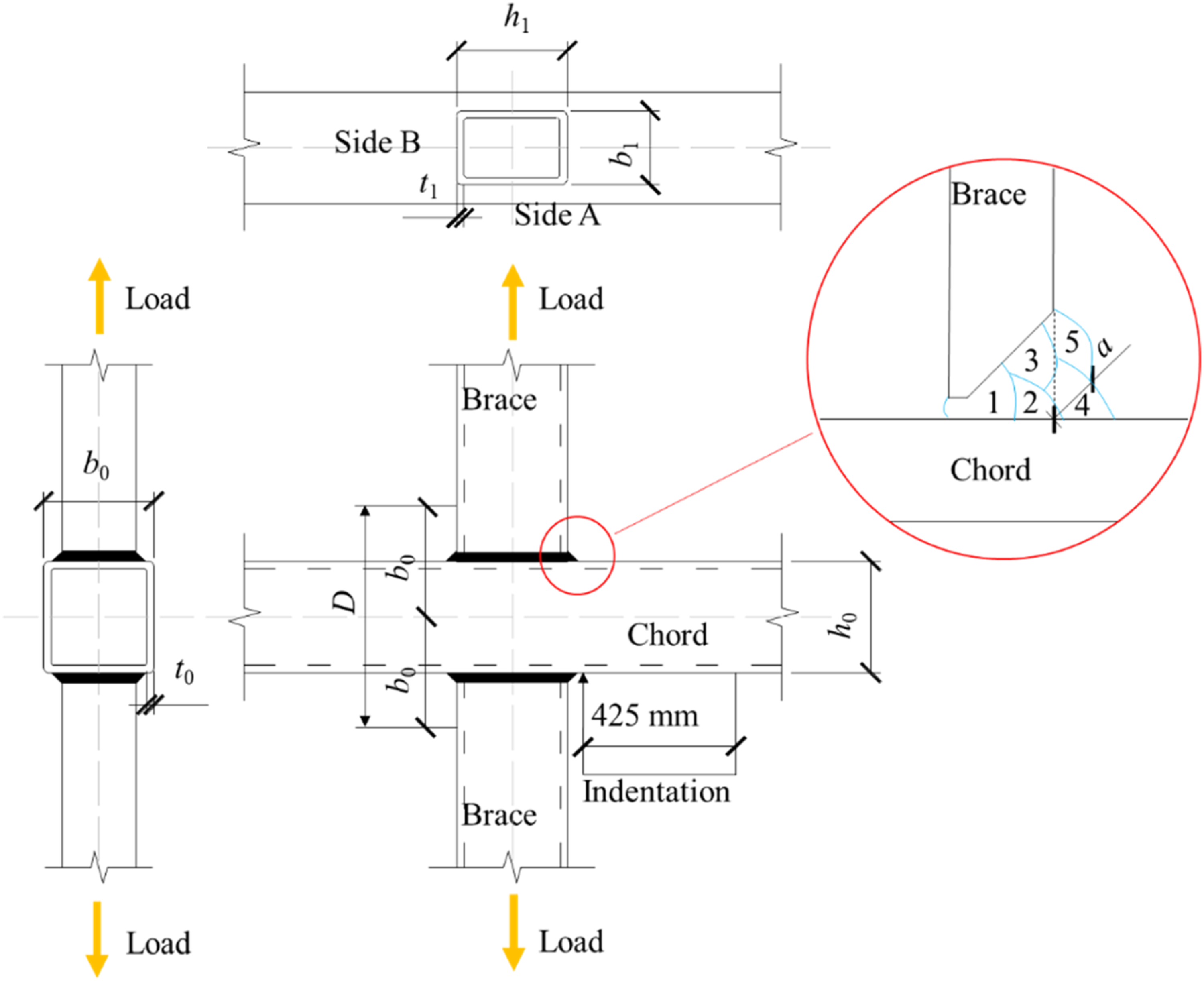
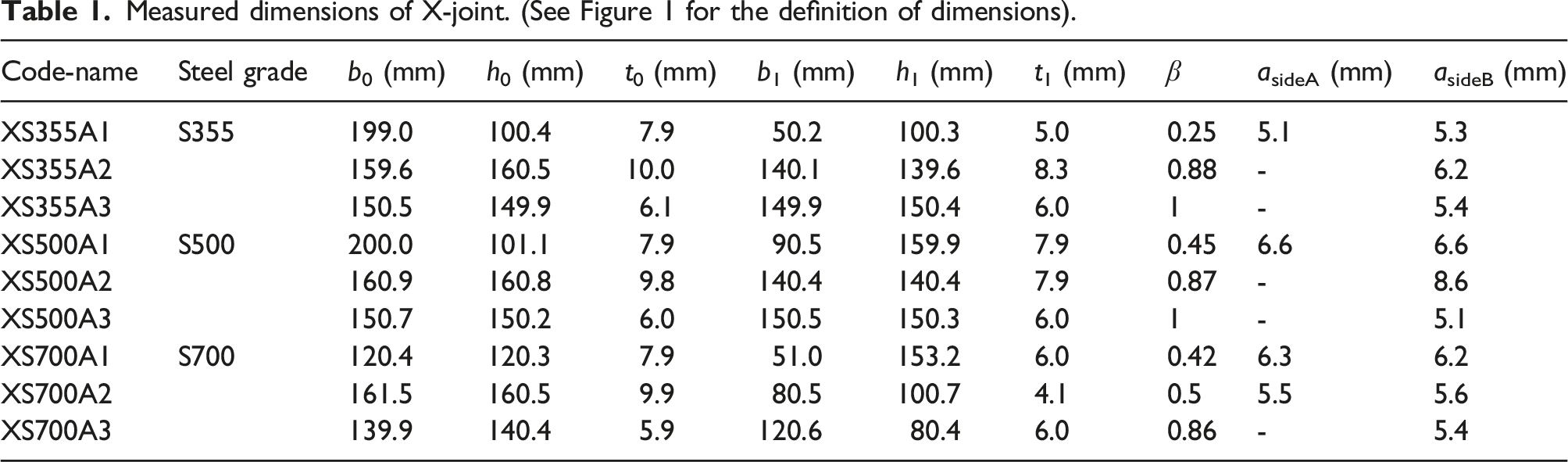
Measured dimensions of X-joint. (See Figure 1 for the definition of dimensions).
A workshop proficient in welding HSSs was employed to carry out to fabricate the specimens using their own welding procedures. The main reason for employing an industrial workshop rather than performing the welding in laboratory conditions was to emulate a welding conditions used in practice. The filler metal Carbofil 1 was used for S355 joints, whereas S500 and S700 joints were welded by Union NiMoCr. The workshop reported the minimum preheat temperature, the maximum interpass temperature, and the heat input of the metal active gas (MAG) welding process were 20°C, 200°C, and 1–1.4 kJ/mm, respectively. Other welding parameters were not provided.
The tensile tests were conducted in two testing setups. Specimens XS355A1, XS500A1, XS500A2, XS500A3, and XS700A1 were tested in a 2 MN setup, while the rest of the specimens were tested in a 10 MN setup. The longitudinal deformation of the specimen was measured using 4 Linear Variable Differential Transformers (LVDTs) based on a 2b0 initial gauge length, as shown in Figure 2. For more details of the experiments and results, see (Yan et al., 2022a). Measurements of X-joint tests.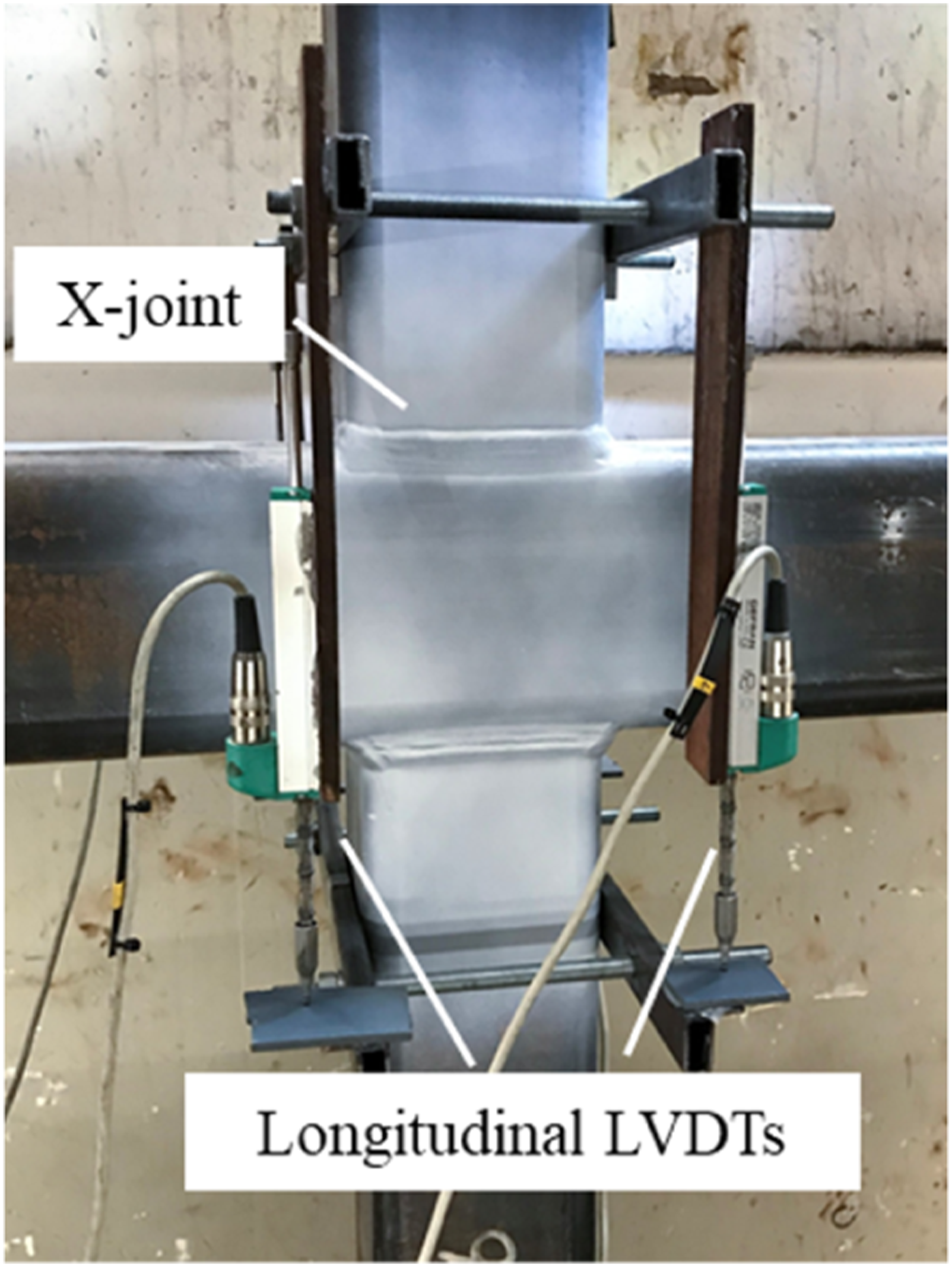
Tensile coupon tests
Standard coupon specimens were fabricated from the wall opposite the longitudinal weld of RHS in X-joints, as shown in Figure 3(a), to obtain the stress-strain relationship of BM. The initial gauge length of the coupon test was 50 mm based on a 5.65 proportional coefficient (Metallic materials - Tensile testing - Part 1: Method of test at room temperature, 2019). Coupon specimens for BM and HAZ. (a) Standard coupon specimen cutting scheme, (b) Welded coupon specimen cutting scheme.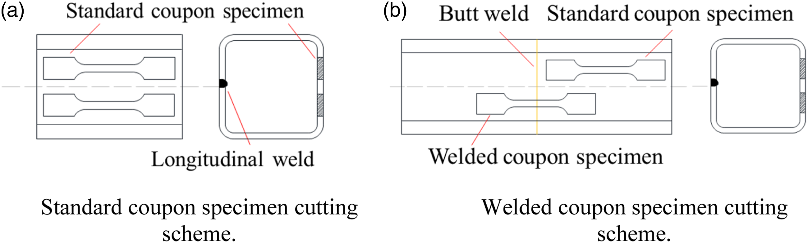
In addition, nine cold-formed RHS profiles, from the same batch as the profiles used for the X-joints, were employed to obtain the stress-strain relationship of HAZ concerning three steel grades (S355, S500, and S700) and three thicknesses for each steel grade (4 or 5 mm, 8 mm, and 10 mm). Two short pieces, 200 mm long, of the hollow section were welded by a single-V full penetration butt weld, as shown in Figure 4. The name of the welded short tube consists of the steel grade and the thickness. For example, S700t8 represents the profile with S700 steel grade and a 8 mm thickness. The same welding parameters and filler metals used for the X-joints were adopted for welding the short profiles. Welded tubes. (a) S355t5. (b) S355t8. (c) S355t10. (d) S500t4. (e) S500t8. (f) S500t10. (g) S700t5. (h) S700t8. (i) S700t10.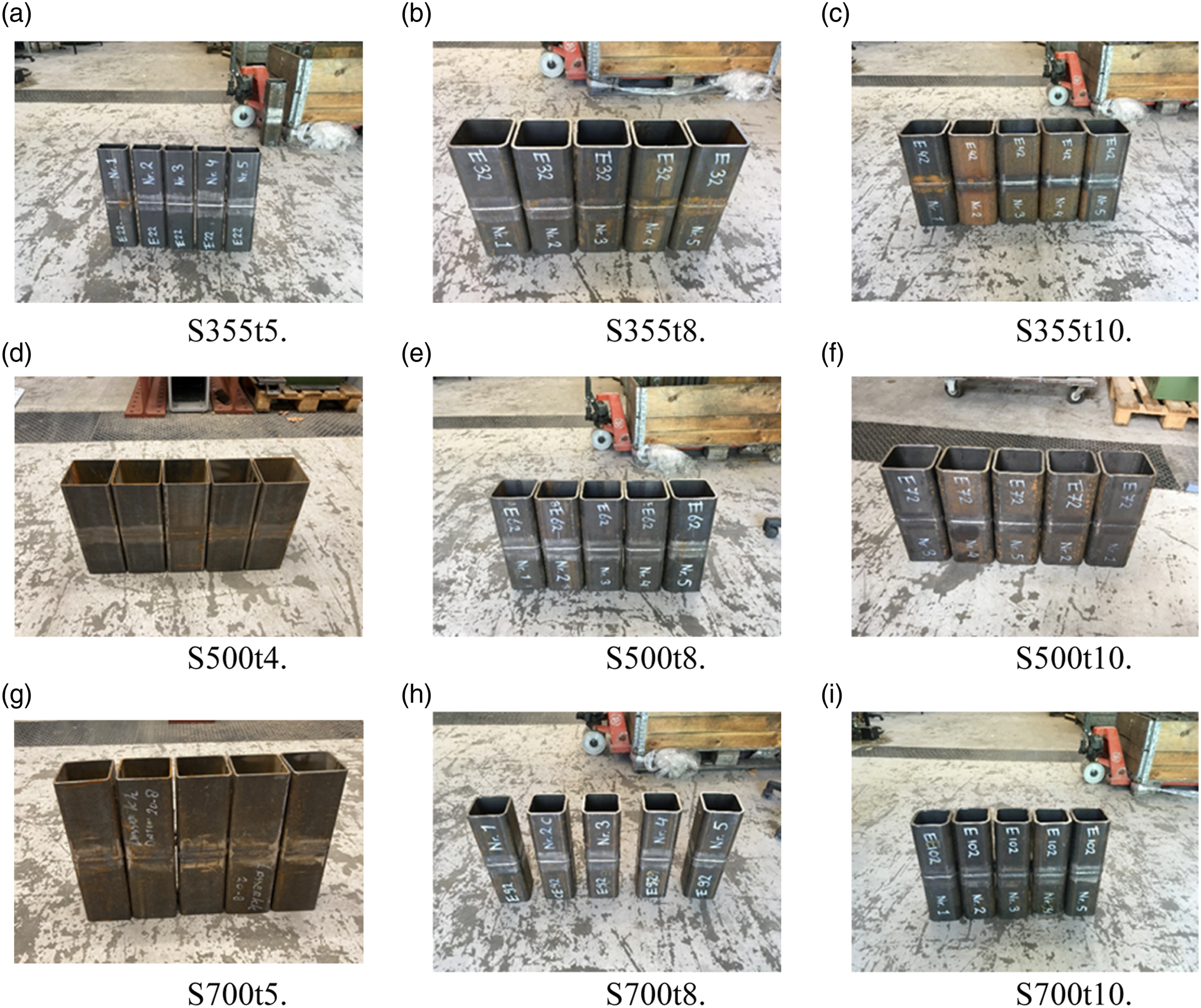
Two types of specimens were cut out from the flat wall of the tube opposite the side with the longitudinal weld, as shown in Figure 3(b). The standard coupon specimen and the welded coupon specimen were used to obtain the BM and HAZ stress-strain relationships, respectively. The welded coupon specimen was milled to a central thickness zone of 3 mm to have the width of HAZ through the thickness as constant as possible. It is worth mentioning that the milled welded coupon specimen failed in HAZ, such that the complete stress-strain relationship of HAZ, including the softening part, was obtained. Figure 5 presents the coupon test setup. Two monitoring methods were used: an extensometer and a 3D DIC (ARAMIS) to measure the elongation and complete deformation of the specimen, respectively, from two opposite sides of the specimen. An initial bow existed in the standard coupon specimen due to residual stress generated in the tube during the cold-forming process. The deformations measured from two opposite sides were averaged. For the milled welded coupon specimen, the testing result of DIC was used, as the specimen was not curved. Measurements of Coupon tests.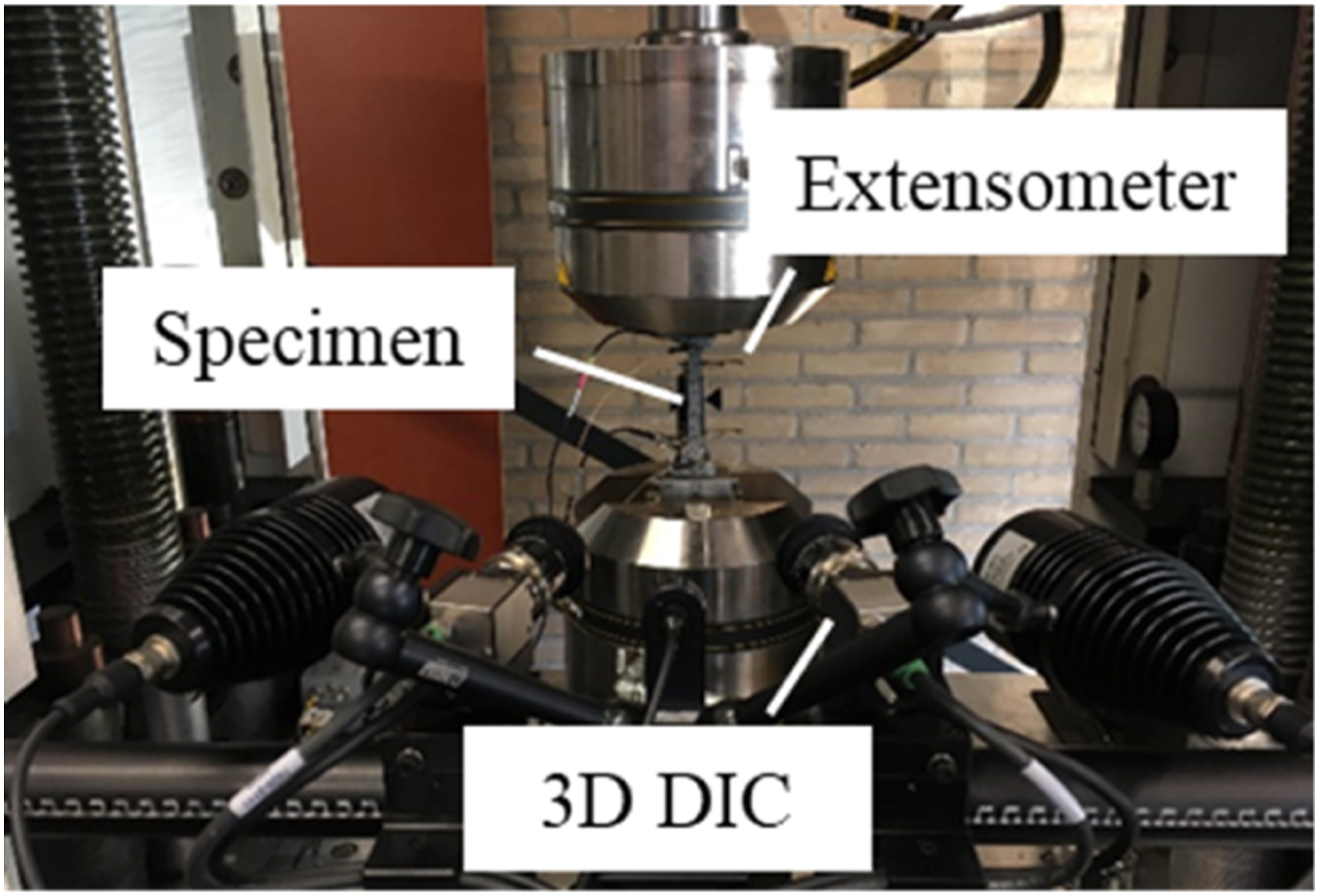
Numerical models
Gurson-Tvergaard-Needleman damage model
The GTN damage model (Tvergaard and Needleman, 1984) is employed to simulate the fracture at monotonic loading in this paper. Equation (1) presents the yield surface of the GTN model. The shape of the yield surface is defined by three parameters q1, q2, and q3, which are calibrated in a homogenization procedure, see Sections ‘Representative volume element models', 'Correlation between VVF and initial hardening strain', and 'Yield surface parameters (q1 and q2)' below. σm and σeq are the hydrostatic pressure, see equation (2) and the von Mises equivalent stress, see equation (3), respectively. σy is the flow stress of the undamaged material matrix.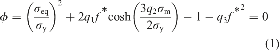
The existing void would grow accompanying the plastic deformation according to the volume preservation assumption. The increment of the void growth (

The expression of the modified VVF (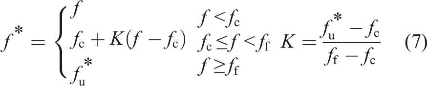
Undamaged true stress-true strain relationship
The undamaged true stress-true strain relationship consists of pre- and post-necking parts. The pre-necking part is obtained from the tensile coupon test by converting the engineering stress-strain relationship until the ultimate strength to the true stress-strain relationship following equation (8).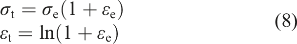


Representative volume element models
The steel material contains voids and steel matrix. It is impossible to create the voids in the coupon specimens or in the welded joints, as the extremely small voids results in meshing and computation efficiency problems. Hence, the voids are created in a unit cell representing a homogenised material, as shown in Figure 6. The mechanical response of the homogenised material is obtained by varying boundary conditions. Accordingly, some constitutive parameters, such as q1 and q2 in this paper, could be determined based on the simulation results. This simulation procedure is called the computational homogenisation analysis. An example of the representative volume element model.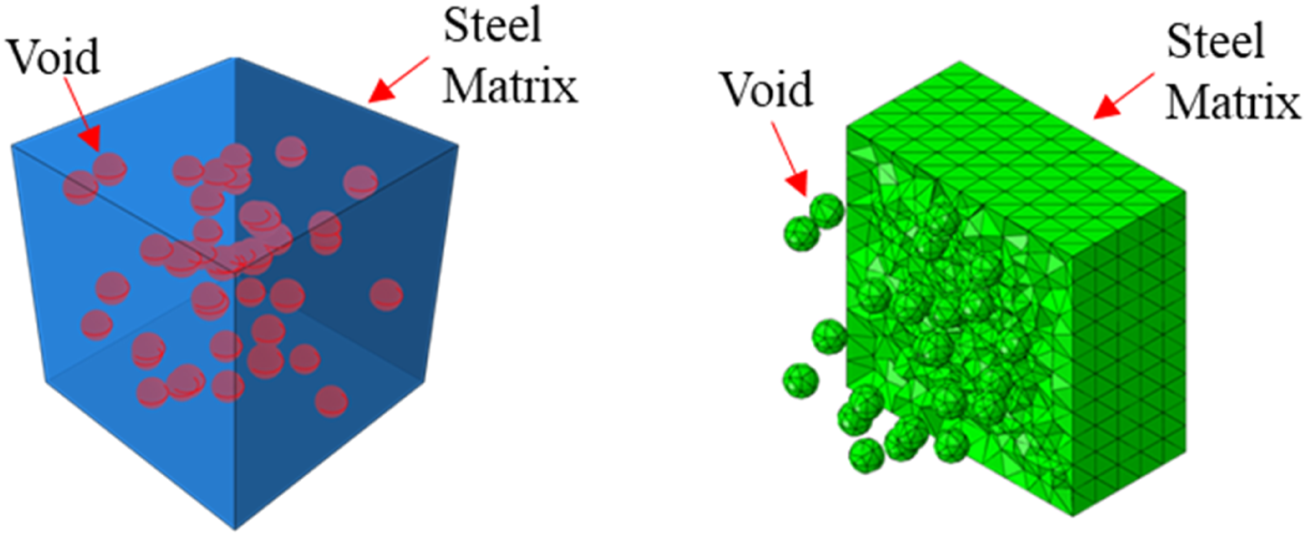
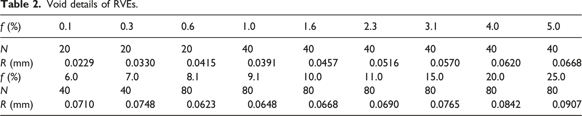
Void details of RVEs.
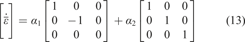
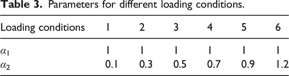
Parameters for different loading conditions.
Coupon specimen models
FE models are created based on the measured dimensions for the standard coupon specimen and the milled welded coupon specimen to calibrate the GTN parameters for BM and HAZ, as shown in Figure 7. The welded coupon specimen contains two HAZ zones and one WM zone. The width was determined using the method proposed by Yan et al., 2021a, 2022c. The FE models finely mesh with 0.5 mm element size in the central part 50 mm long, the base length where the extensometer was installed. The remaining part uses a coarse mesh in the loading direction. In order to reduce the computational burden, the grip part of the specimen is not created. Two reference points, RP1 and RP2, are employed to control all three translations and three rotations of the end surfaces using the multi-point beam constraint (MPC beam). A positive displacement in the Y direction is applied at RP2, while the other degrees of freedom of RP1 and RP2 are fixed. The explicit solver with a 100 s period and a 0.0001 s target time increment is used to perform the quasi-static analysis. Eight-node hexahedral solid elements with reduced integration (C3D8R) are employed in the model. Finite element model of coupon specimens. (a) Standard coupon specimen. (b) Milled welded coupon specimen.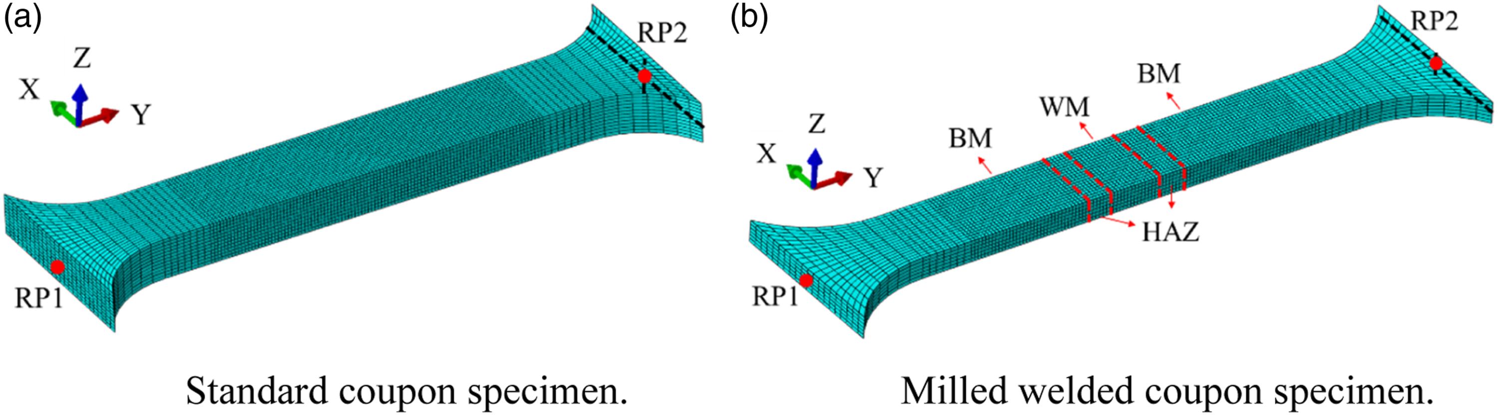
X-joint models
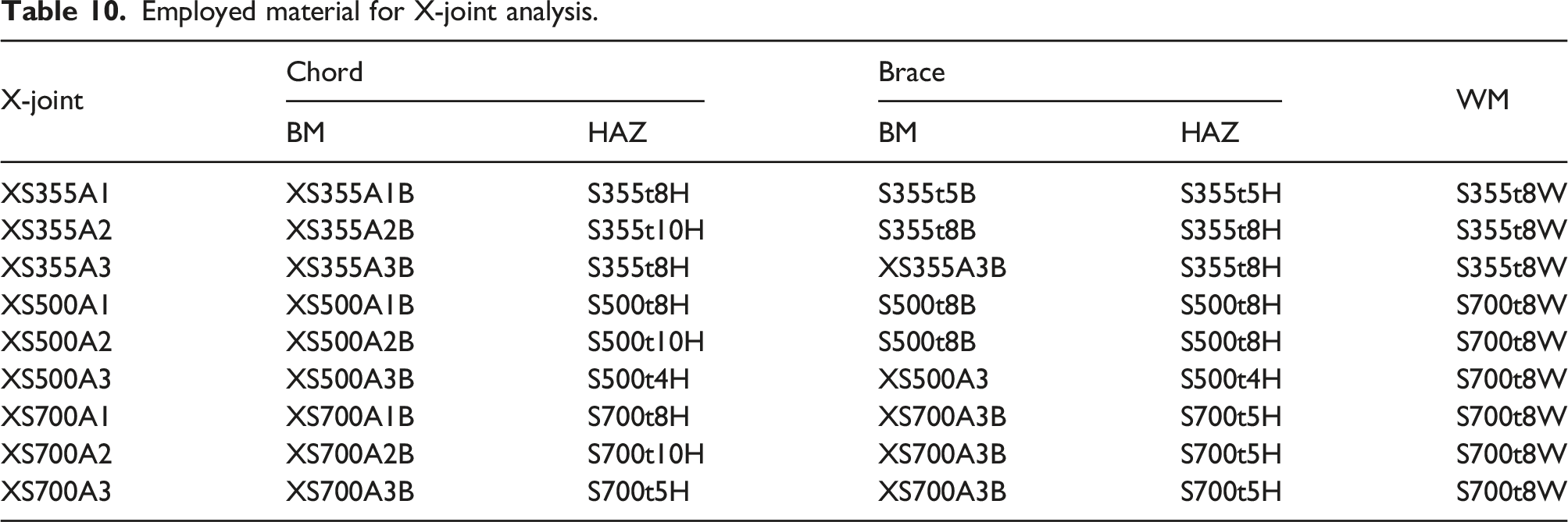
FE models are generated to verify the GTN damage model and the experiments. The models are built up with the measured geometric dimension, as shown in Table 1. Only a quarter of the joint is created to reduce the computational burden. Figure 8 shows an example of the FE model for the specimen XS500A2. Reference points (RP1 and RP2) are made at the centre of the entire RHS end surfaces (marked with yellow). Each reference point controls all translations and rotations of the corresponding end surface through the MPC beam constraint. The loading is applied as a positive displacement at RP1 in the Y direction. The remaining degrees of freedom at reference points are fixed. In addition, symmetry boundary conditions are applied on Surface 1 and Surface 2, see Figure 8. The quasi-static analysis is conducted using the explicit solver with a 100 s period and a 0.0001 s target time increment. Finite element model for X-joints.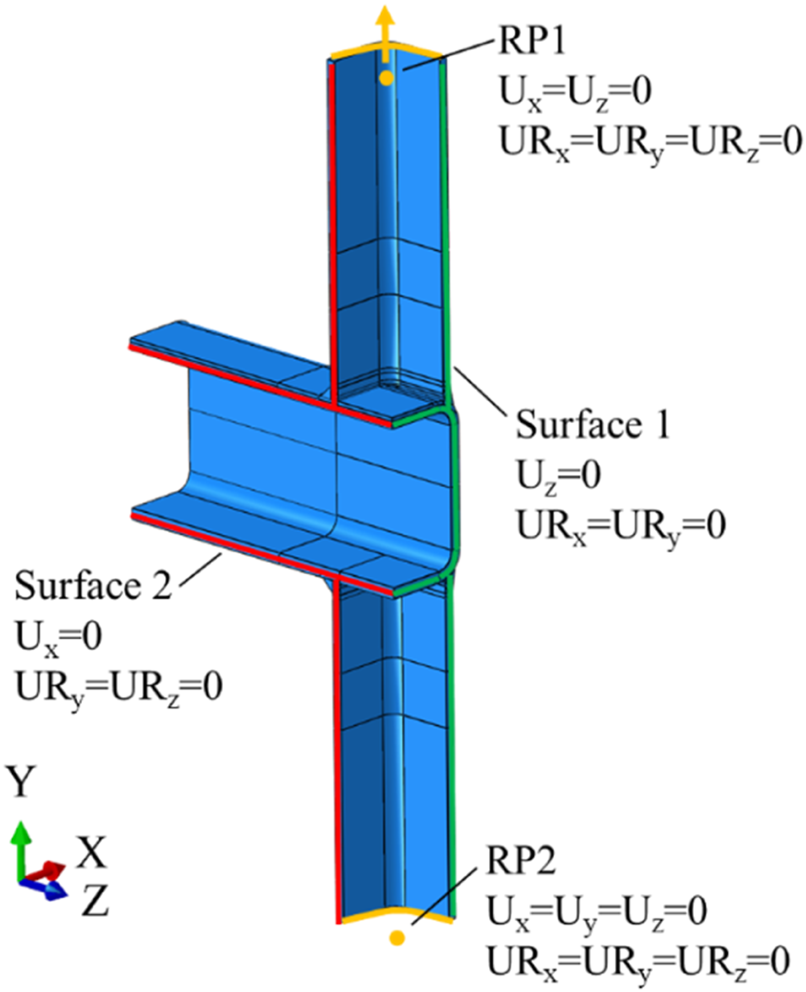
The weld zone consists of five material regions: Chord, Chord HAZ, WM, Brace, and Brace HAZ. Figure 9 shows the HAZ and WM regions in the FE model. The HAZ width in the butt welded tubes, referring to Figure 3(b), is measured based on the Vickers hardness tests (Yan et al., 2022b. It was found that the majority (92%) of the HAZ width varies between 2 mm and 4 mm, with an average 3.2 mm width regardless of the steel grade and the thickness of the profile. Hence, a 3.2 mm HAZ width is used in all X-joint models. The HAZ region in the brace is oriented parallel to the bevelled surface, while the HAZ in the chord is oriented through the thickness of the cross-section. HAZ and WM regions in a weld zone.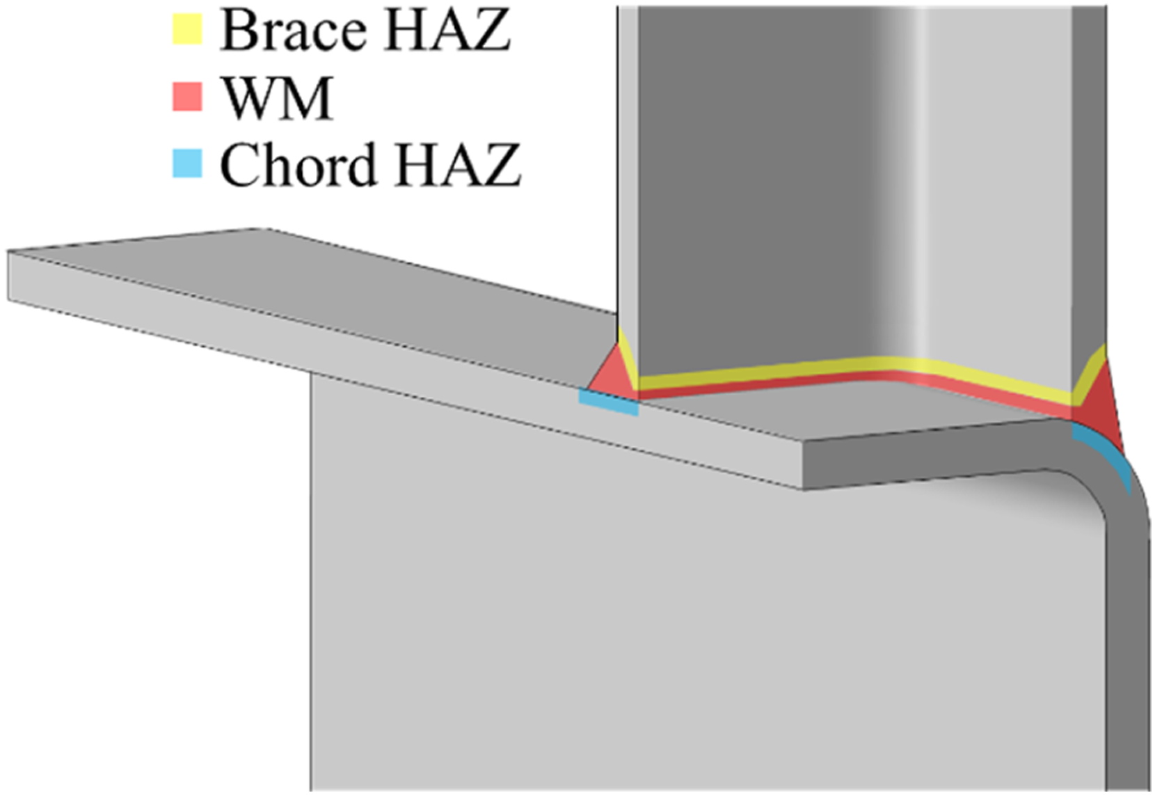
The C3D8R element is used for modelling joints with β < 0.8, i.e. the joints XS355A1, XS500A1, XS700A1, and XS700A2 (see Table 1). A 0.5 mm mesh size is adopted for critical regions concerning HAZ, WM, and part of BM close to HAZ. The BM mesh size along the profile length direction gradually changes to 5 mm. Due to the complex geometry at the chord corner of joints with β > 0.8 (XS355A2, XS355A3, XS500A2, XS500A3, and XS700A3), it is not possible to mesh using the C3D8R element. The ten-node tetrahedral element C3D10 is employed. A universal 1 mm mesh size is used for HAZ, WM and part of BM close to HAZ. Note that the chord front face of XS355A3 also meshed with 1 mm elements as a chord side wall failure (CSWF) appeared in the experiment. Two examples of FE mesh using C3D8R and C3D10 elements are presented in Figure 10(a) and (b), respectively. Examples of mesh used in the FE models. (a) XS700A1 with the C3D8R element. (b) XS500A2 with the C3D10 element.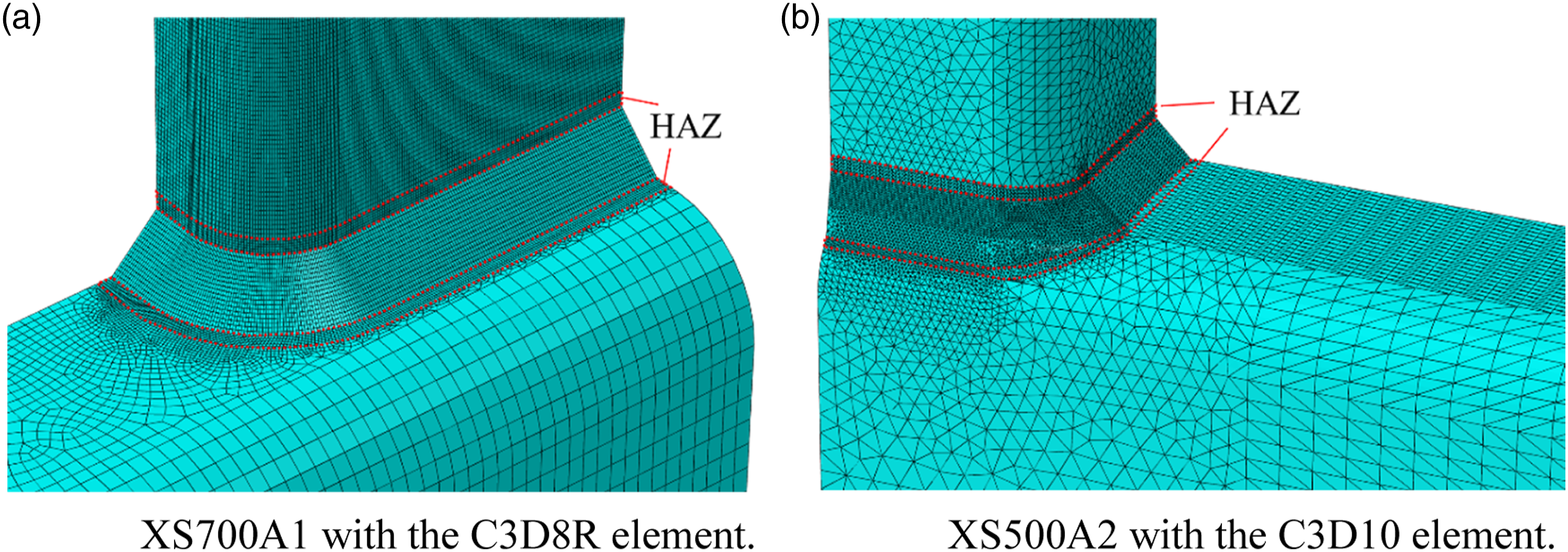
Calibration of GTN parameters
Correlation between VVF and initial hardening strain
The input data (stress-strain relationship) in the RVE model is considered the constitutive model of the steel matrix, excluding the effect of the void on the stress-strain relationship of the material. The RVE model contains the steel matrix and the void, representing a material unit in the real specimen. It can be used to simulate the behaviour of the material unit under different loading conditions and various stages of damage. Hence, the mechanical response of the material unit under different stress states could be obtained from the RVE model. It is assumed that the volume of the steel matrix is unchangeable, indicating that the volume of the homogenised material may change during loading, as the void volume changes. Hence, the plastic hydrostatic strain rate, see equation (5), is not zero.
With different stress triaxialities, the evolution of the plastic strain component is different. Take two sets of the plastic strain increment with the same plastic hydrostatic strain rate (0.003) for instance. The first set of the plastic strain rate is 0.011, 0.001, and −0.009 for True stress-strain relationship with different initial hardening strains.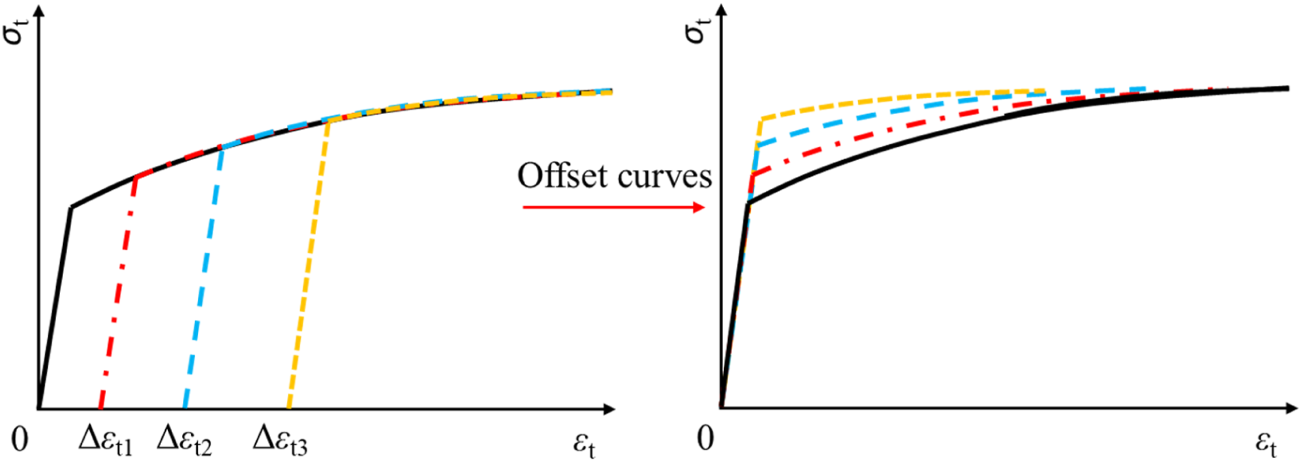
A given VVF corresponds to a range of equivalent plastic strain instead of a unique value. An iteration analysis is conducted based on the RVE model to find the relationship between the range of the accumulated initial hardening strain and a specific VVF. The BM of the XS700A2 chord, denoted XS700A2B, is employed here for illustration. First, the original true stress-strain relationship is used in the RVE model with 0.1% VVF. For the model loaded with a minimum (α2 = 0.1) stress triaxiality, the equivalent plastic strain and VVF at the yield point are 0.062% and 0.258%, respectively. The model loaded with a maximum (α2 = 1.2) stress triaxiality has a 0.00382 equivalent strain and 0.343% VVF at the yield point. Comparing the results of the two models, VVF has a limited variation while the equivalent strain shows a significant difference. Hence, an RVE model with 0.3% VVF, which is approximately the average of two VVFs at the yield point (0.258% and 0.343%), is created for the second step analysis. As 0.062 and 0.00382 are the maximum and minimum equivalent plastic strains that may appear in the material with 0.3% VVF, the strains are used as the initial hardening strain (see Figure 11) to modify the original true stress-strain relationship. Note that the maximum and minimum initial hardening strains are slightly adjusted within the varying range to have simple numbers. In addition, the average of the maximum and minimum initial hardening strain is used to generate a moderate constitutive model. The three modified stress-strain relationships are used in the second step analysis.
The model using the stress-strain relationship modified by the maximum initial hardening strain has the highest equivalent strain at the yield point under the α2 = 0.1 loading condition, while the model using the minimum-strain modified stress-strain relationship has the lowest equivalent yield strain under the α2 = 1.2 loading condition. VVF of these two models at the yield point shows a slight difference (0.554% and 0.663%). The average of two VVFs (approximately 0.6%) is used to create the RVE model for the third step. Similar to the first step, the original stress-strain relationship is modified using the accumulated initial hardening strain, which is the sum of maximum (or minimum) initial hardening strains. Again, a moderate modified constitutive model is created using the average of the maximum and minimum accumulated initial hardening strains.
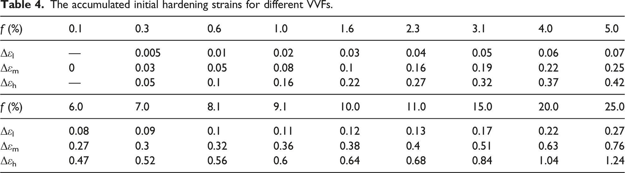
The accumulated initial hardening strains for different VVFs.
Yield surface parameters (q1 and q2)
An example of the RVE simulation result concerning a 5% VVF, a 0.07 accumulated initial hardening strain, and the Swift model extrapolation is presented in Figure 12. The equivalent stress-strain relationship is used to characterise the yielding of the RVE model. When the slope of the curve decreases to 1% of the initial elastic stiffness, the point is considered the yield point. Figure 12(b) illustrates the pressure dependence of the yield surface, where the von Mises yield stress decreases with the increase of the mean stress. Example of RVE results (f = 5%, 0.07 strain hardening, Swift model extrapolation). (a) σ
eq
-ε
eq
relationships. (b) σeq-σm relationships.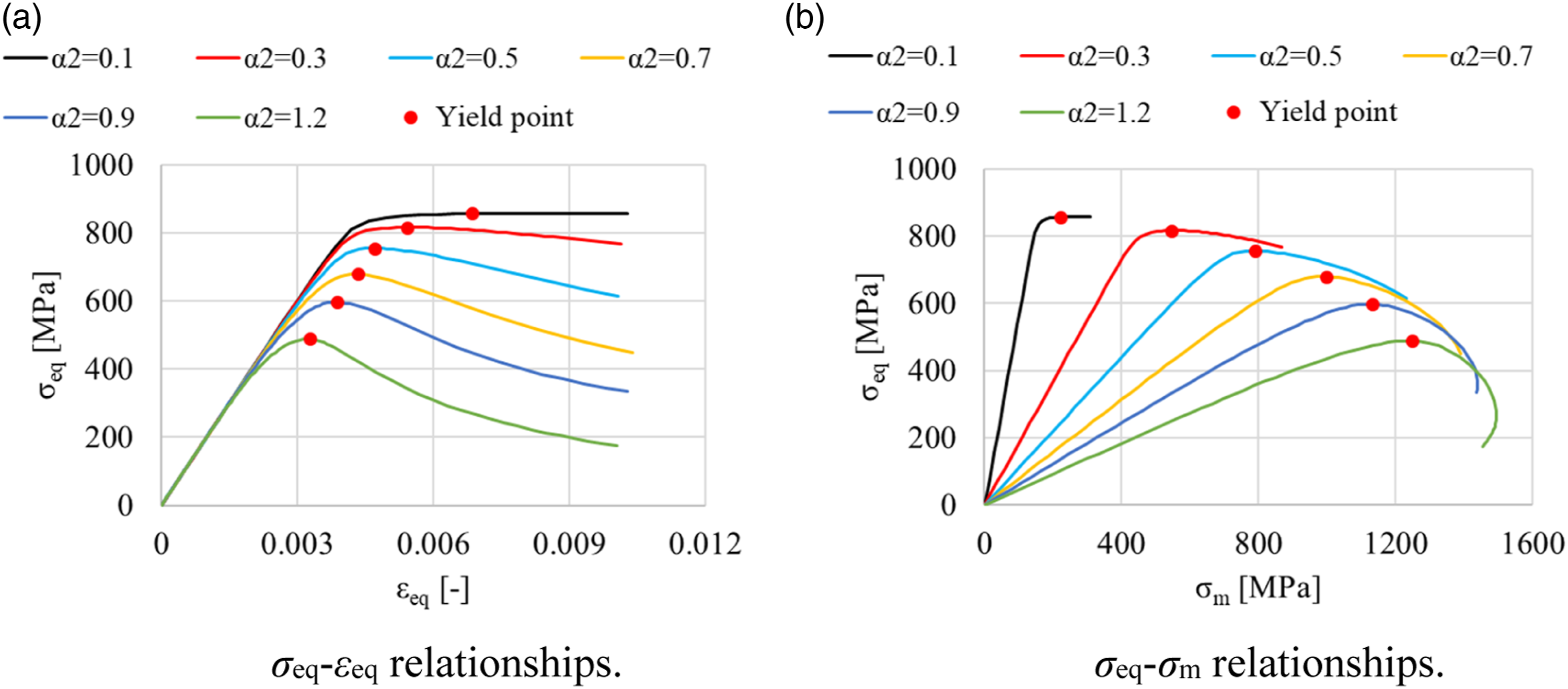
Calibrated parameter q1.
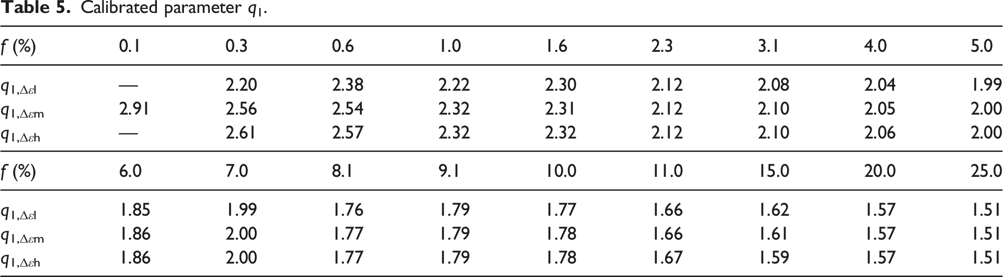
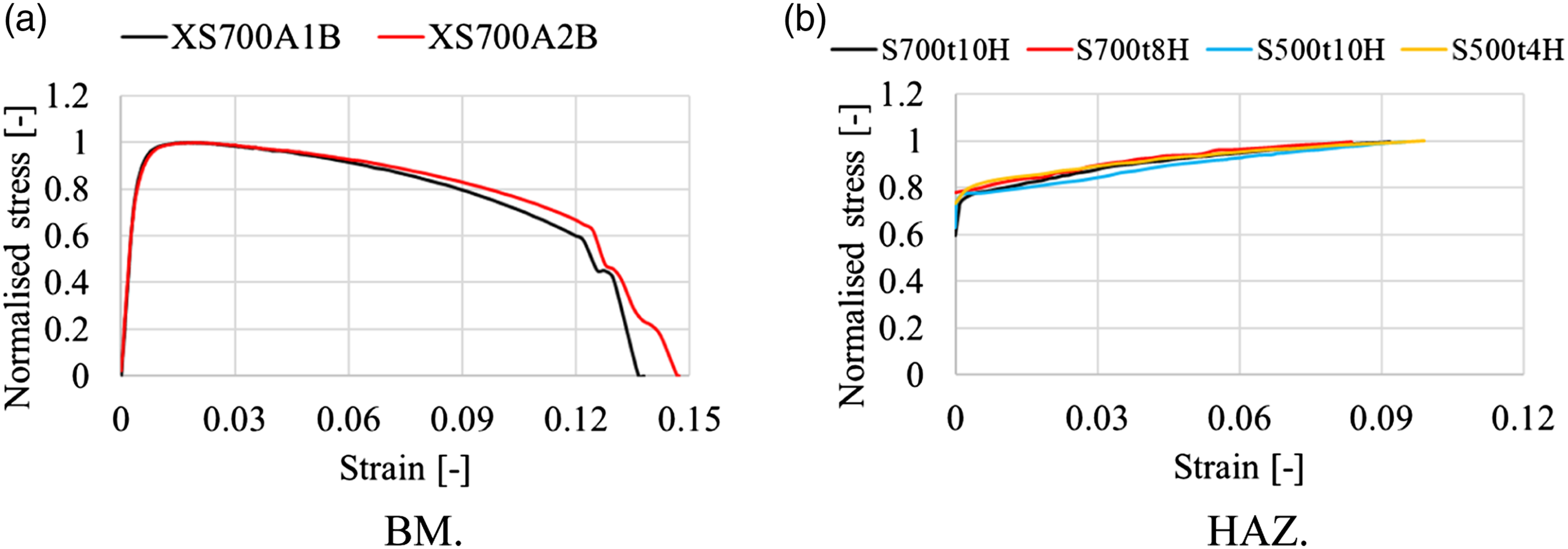
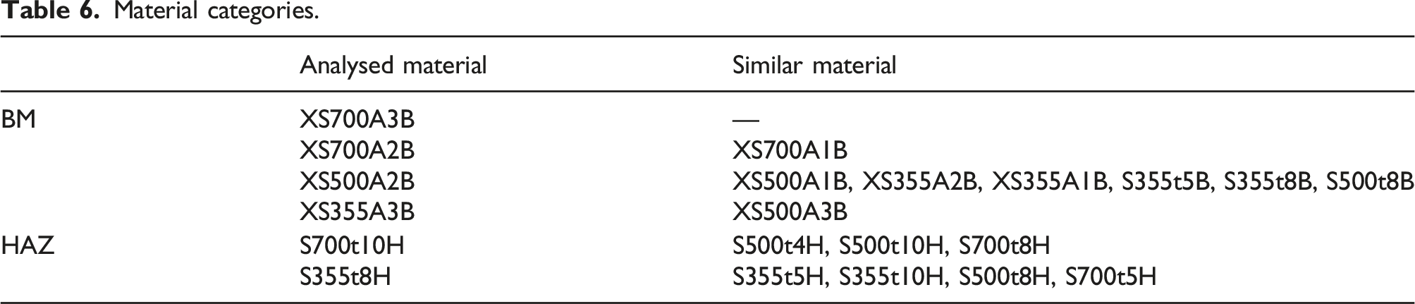
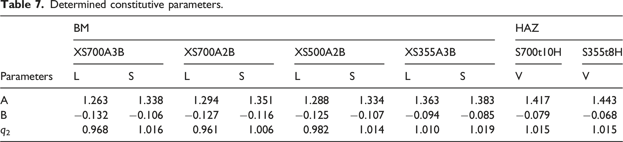
Fritzen et al. (2012) found that q1 decreases with an increasing VVF and a constant q2. An expression correlating q1 and VVF proposed by Yan et al. (2021b) is adopted in this work, as presented in equation (14). Materials with a similar strain hardening behaviour. (a) BM. (b) HAZ. Material categories.
Determined constitutive parameters.
Fracture parameters (fc and ff)
The undamaged true stress-strain relationship is used in the coupon specimen analysis. The pressure-dependent yield surface of the GTN model is realised by the porous metal plasticity in ABAQUS. A user subroutine VUSDFLD, as introduced in (Yan et al., 2021b), is used to consider the relationship between q1 and VVF. The initial VVF f0 is 0.001, resulting in a 0.999 relative density.
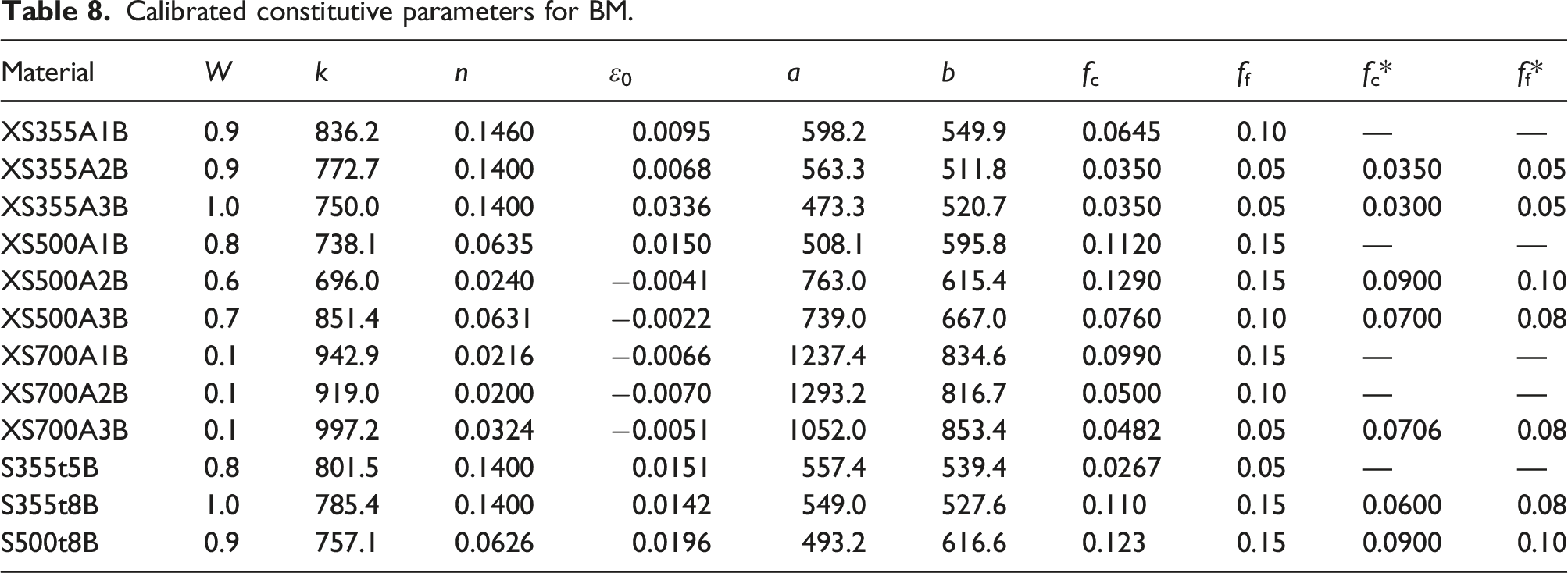
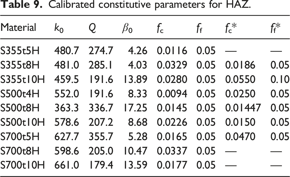
Figure 14(a) presents the engineering stress-strain relationship of XS700A3B. The solid black line is the experimental result. The results of FE1, FE2, and FE3 are extracted from the FE model with a 0, 0.1, and 0.2 weighting factor referring to equation (12), respectively. The FE model with a 0.1 weighting factor fits the experimental result best. The VVF contour plot of the half FE model at the failure point, where the load decreases sharply, is presented in Figure 14(b). It can be seen that the highest VVF appears at the centre of the cross-section, indicating the fracture initiates from the centre. The maximum VVF is taken as fc. The value of ff is determined based on a trial-and-error process by varying ff. Figure 14(c) compares the experimental and the FE results, where FE2-1, FE2-2, and FE2-3 use 0.05, 0.1 and 0.15 ff, respectively. The model FE2-1 with a 0.05 ff fits the experimental result best, although a minor difference could be observed among all three FE results. Note that the FE model with an ff smaller than the proposed value would not notably influence the stress-strain relationship obtained from the FE result. Hence, an ff which is maximally 0.05 larger than fc is adopted in this study. The parameters calibrated for BM (referring to equation (10)) and HAZ (referring to equation (9)) are summarized in Table 8 and Table 9, respectively. Determination of constitutive parameters. (a) Weighting factor. (b) VVF contour plot at the failure point. (c) fc and ff. (d) Final fracture. Calibrated constitutive parameters for BM. Calibrated constitutive parameters for HAZ.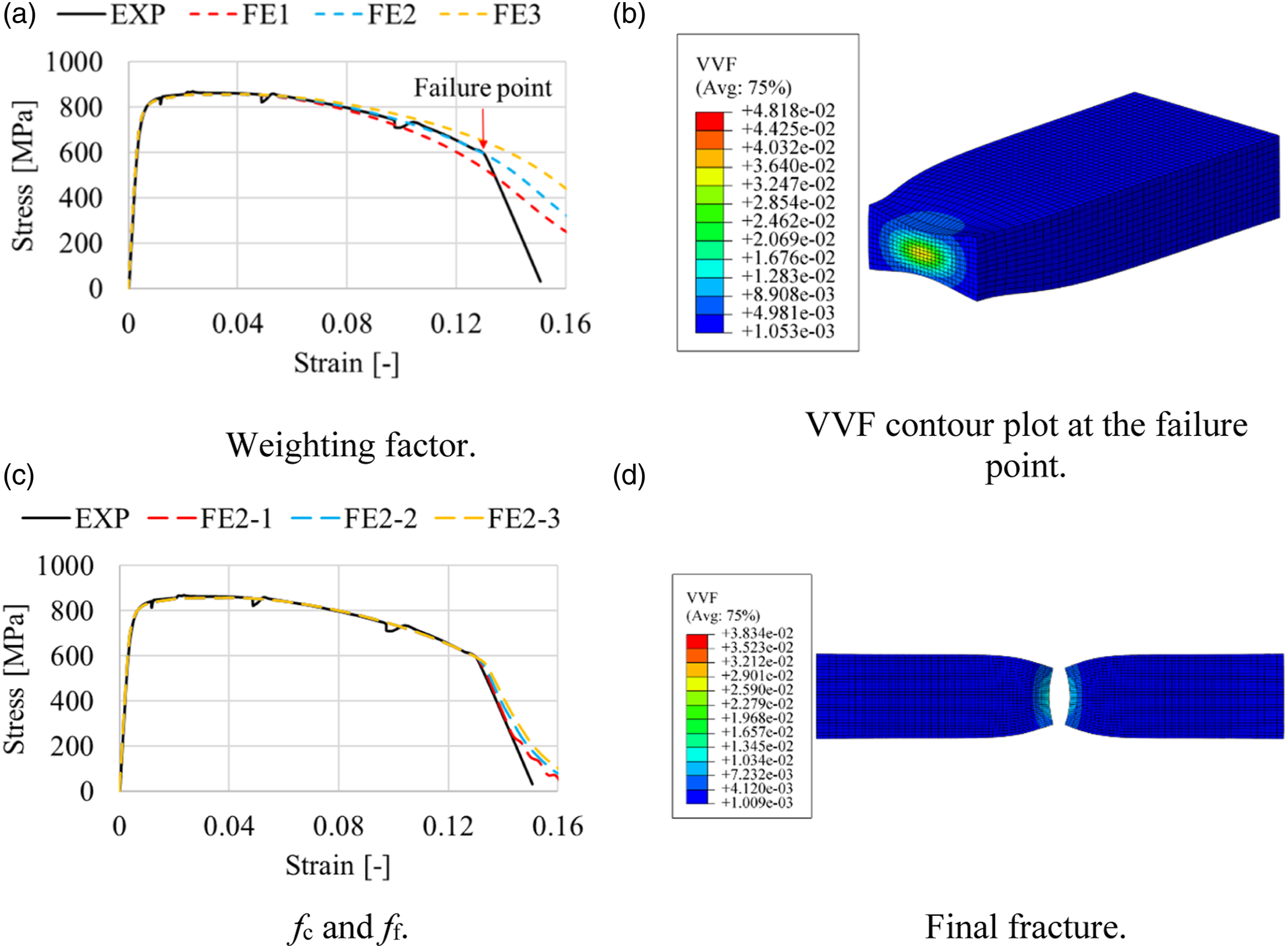
Finite element analysis of X-joints
Employed material for X-joint analysis.
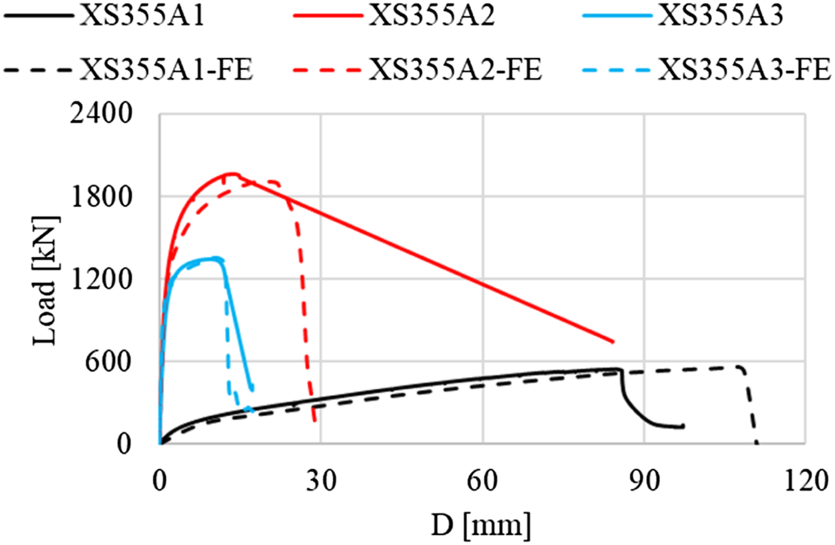
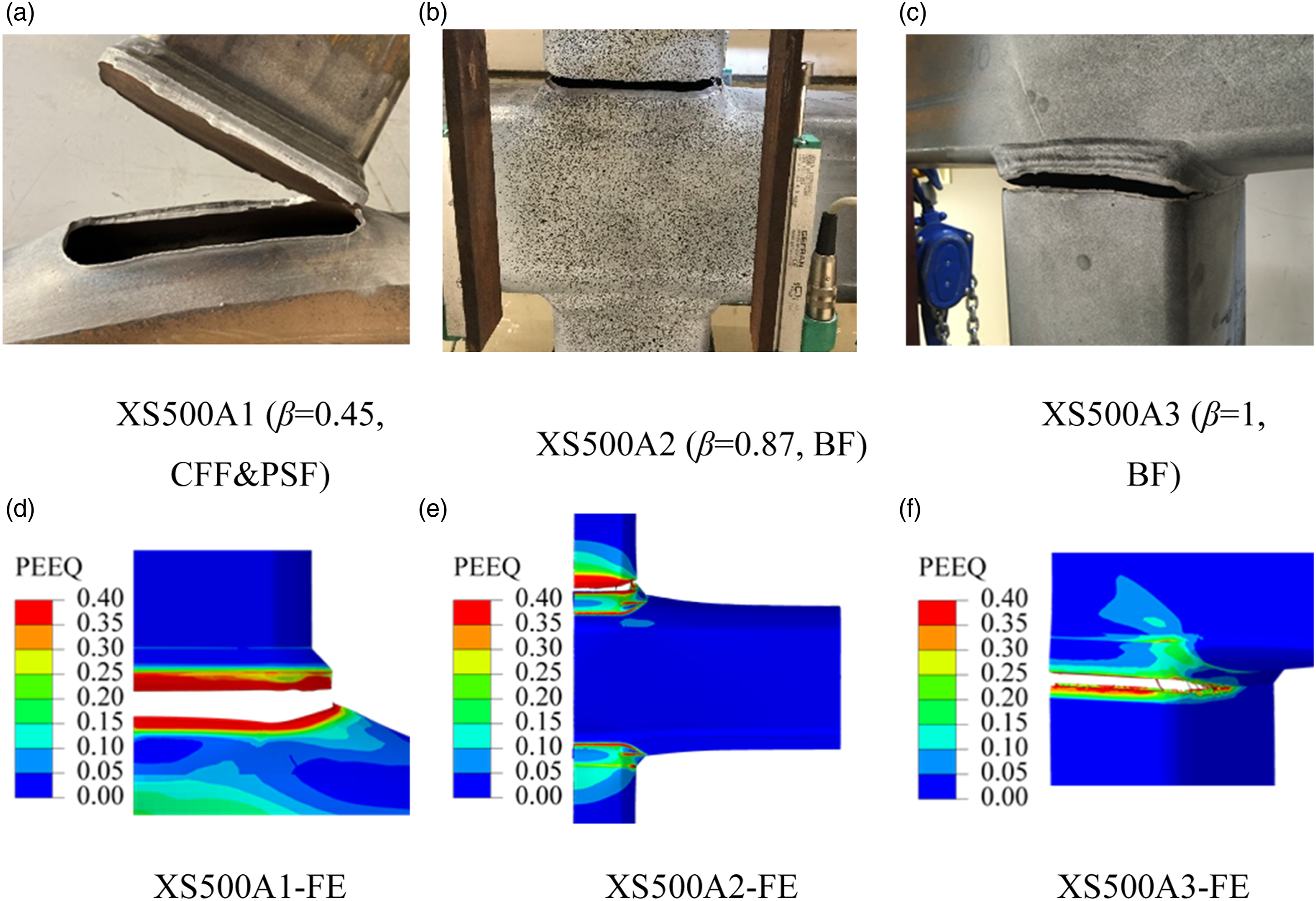
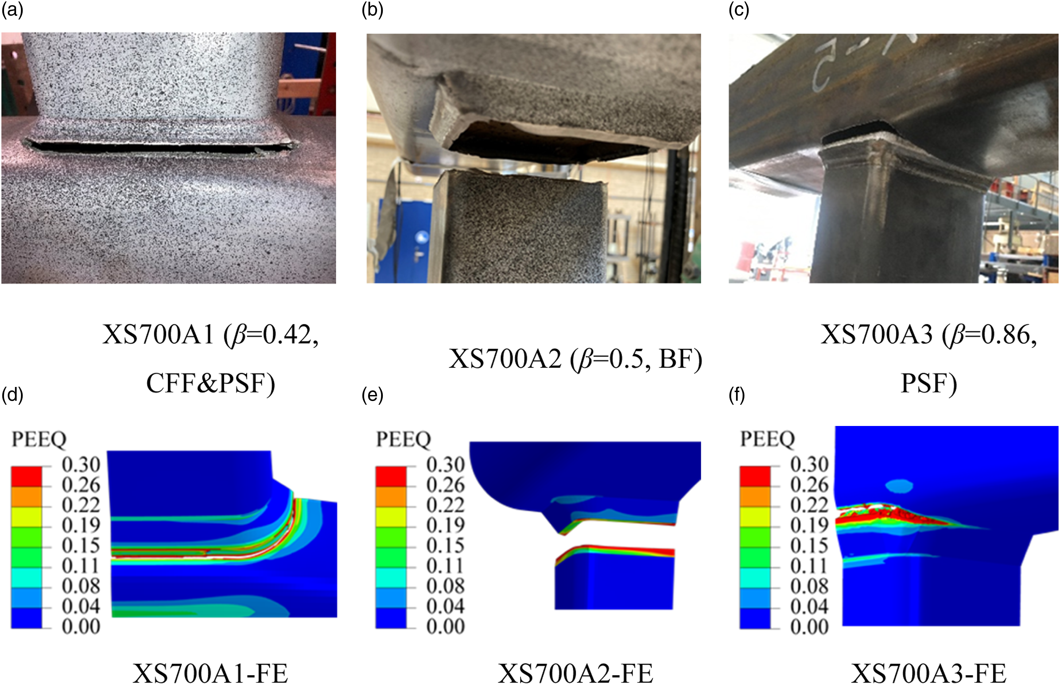
The failure mode and the load-displacement relationship of X-joint FE models are compared to the experimental results in Figures 15 to 20. The predicted load-displacement relationships show a good agreement with the experimental results, although the resistance of FE results is slightly lower than the experiments at the plastic stage, which might be due to the pessimistic assumption of the constitutive model of the corner region in the cold-formed RHS. The material in the corner region has higher strength but lower ductility than the material in the flat region (Wang et al., 2017; Wilkinson, 1999). The absence of the corner material model may also result in a more significant deformation at the ultimate load since the stress concentration is relaxed at the corner region, where the low ductility may lead to a premature fracture. For a joint with a small β, the deformation is mainly due to the deflection of the chord surface, and the role of the corner in the overall behaviour of the joint is less pronounced. For a joint with a large β, the corner region acts more strongly in the load transfer, and the material at the corner undergoes more severe yielding that may lead to failure. Consequently, omitting the work-hardening of the corner region in the material model may have a stronger influence on the FE results for joints with larger β values. In addition, the FE model is only one-quarter of the specimen, and symmetric boundary conditions are applied. The deformation obtained from the FE model may be larger than the experiments, as the fracture appears only on a weaker side of most joints. Failure modes of S355 X-joints. (a) XS355A1 (β = 0.25, CFF&PSF). (b) XS355A2 (β = 0.88, BF). (c) XS355A3 (β = 1, CSWF). (d) XS355A1-FE. (e) XS355A2-FE. (f) XS355A3-FE. Load-displacement relationship of S355 X-joints. Failure modes of S500 X-joints. (a) XS500A1 (β = 0.45, CFF&PSF). (b) XS500A2 (β = 0.87, BF). (c) XS500A3 (β = 1, BF). (d) XS500A1-FE. (e) XS500A2-FE. (f) XS500A3-FE. Load-displacement relationship of S500 X-joints. Failure modes of S700 X-joints. (a) XS700A1 (β = 0.42, CFF&PSF). (b) XS700A2 (β = 0.5, BF). (c) XS700A3 (β = 0.86, PSF). (d) XS700A1-FE. (e) XS700A2-FE. (f) XS700A3-FE. Load-displacement relationship of S700 X-joints.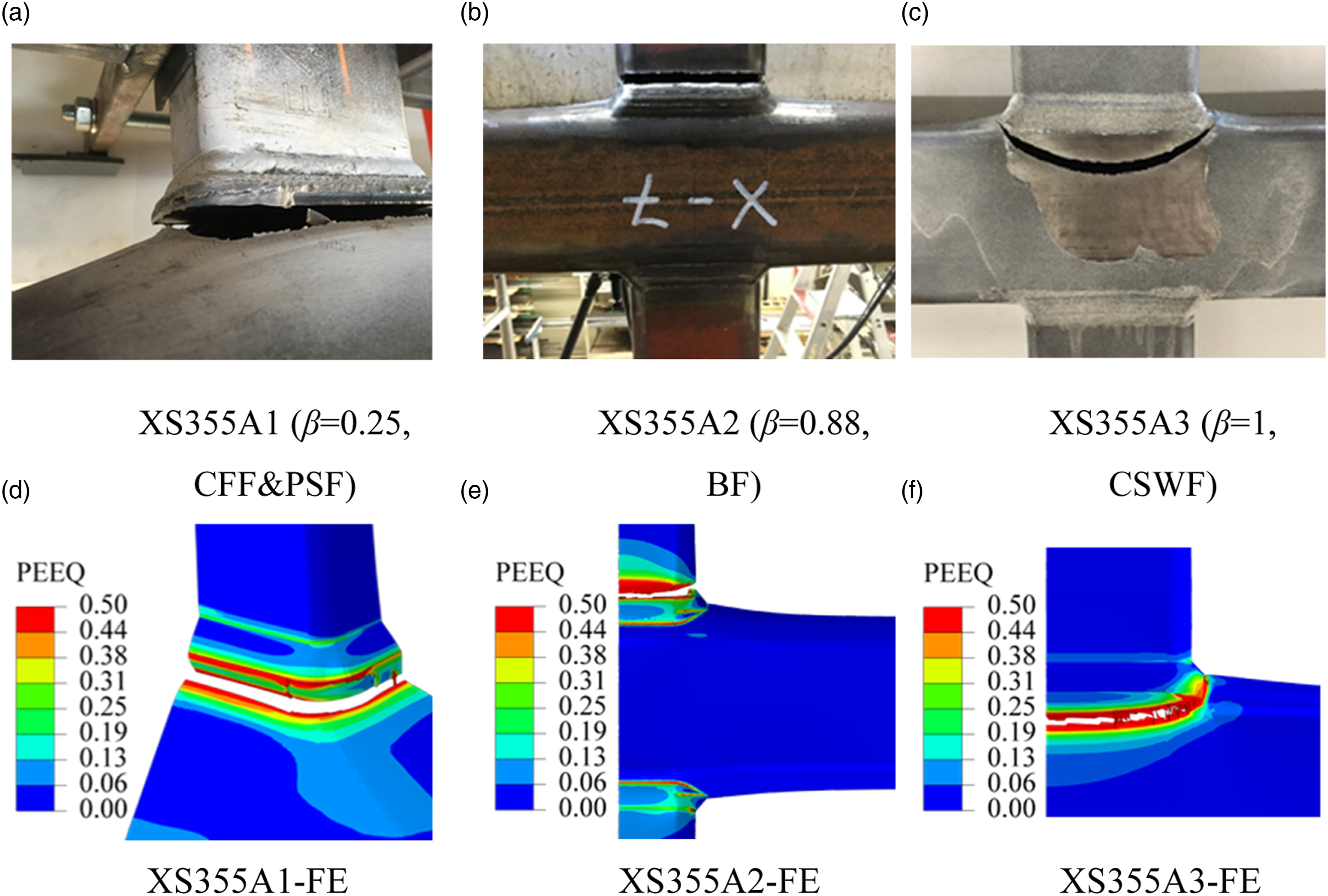
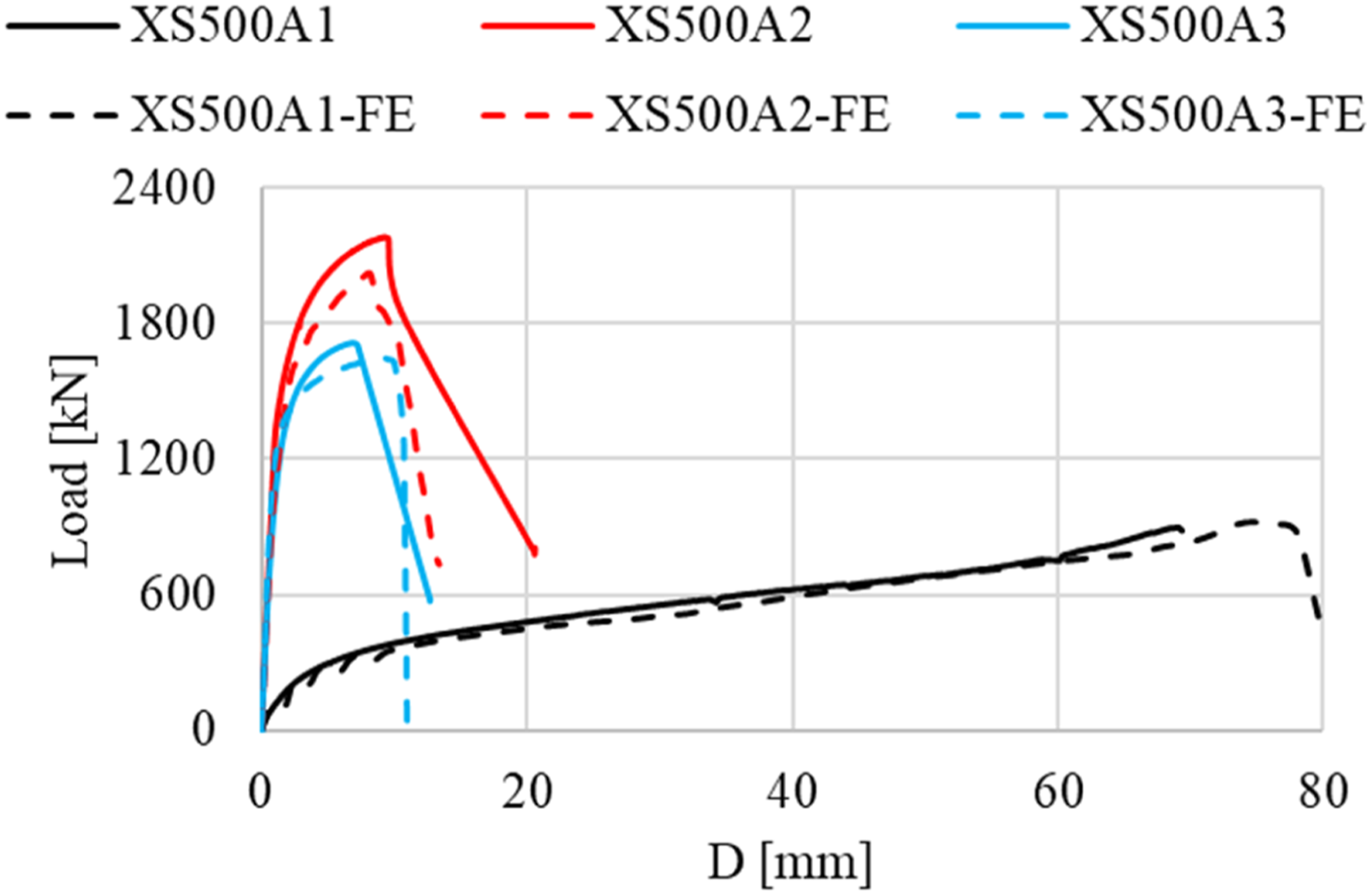
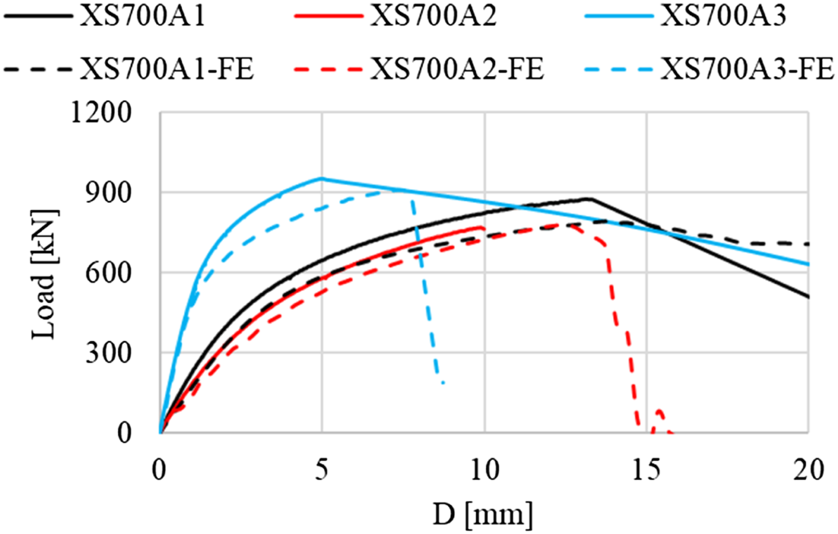
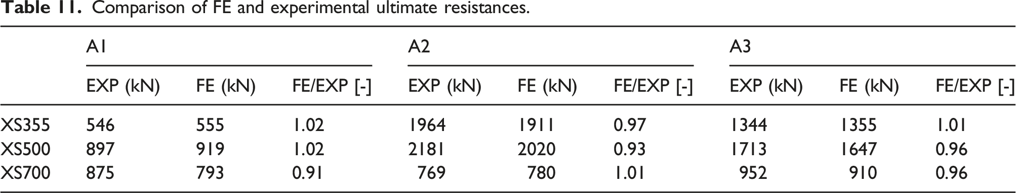
Comparison of FE and experimental ultimate resistances.
The fracture surface of all joints, except for XS700A1, is well predicted using the calibrated GTN damage model. Only XS355A3 had CSWF with an arc-shaped fracture. The FE predicted fracture has a similar shape but is slightly closer to the corner of the chord, which might be due to the absence of the constitutive model of the corner region.
Two orientations of the fracture surface for PSF were observed in the experiments. The fracture of XS355A1, XS500A1, and XS700A3 initiated at the weld toe and cut through the thickness of the tube (see Figure 15, Figure 17, and Figure 19), which is successfully predicted by the FE model. The fracture surface of XS700A1 propagated below the weld, as shown in Figure 21 (solid red line for the experiment and red dash line for the FE model), which fails to predict. Fracture surface in the experiment and FEA of XS700A1. (a) Fracture surface in experiment. (b) Fracture surface in FEA. (c) A sketch of the fracture surface.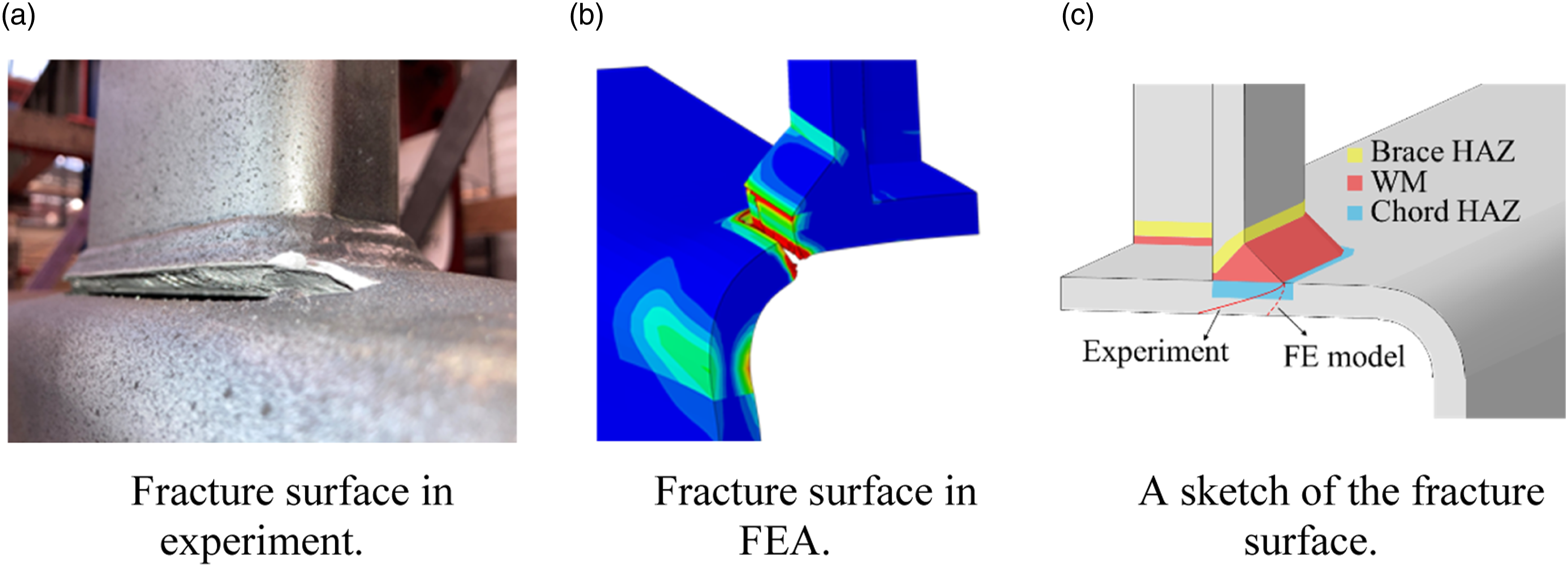
The fractures of all BF have the same orientation, as shown in Figure 14, Figure 16, and Figure 18. A detailed shape of the fracture surface is shown in Figure 22 (a). The normal direction of the fracture surface points out of the X-joint. As the fracture starts from the toe of the weld, the fracture involves HAZ and BM. The FE model successfully predicts the failure mode. Fracture surface in experiments and FEA of XS700A2. (a) Fracture surface in experiment. (b) Fracture surface in FEA. (c) A sketch of the fracture surface.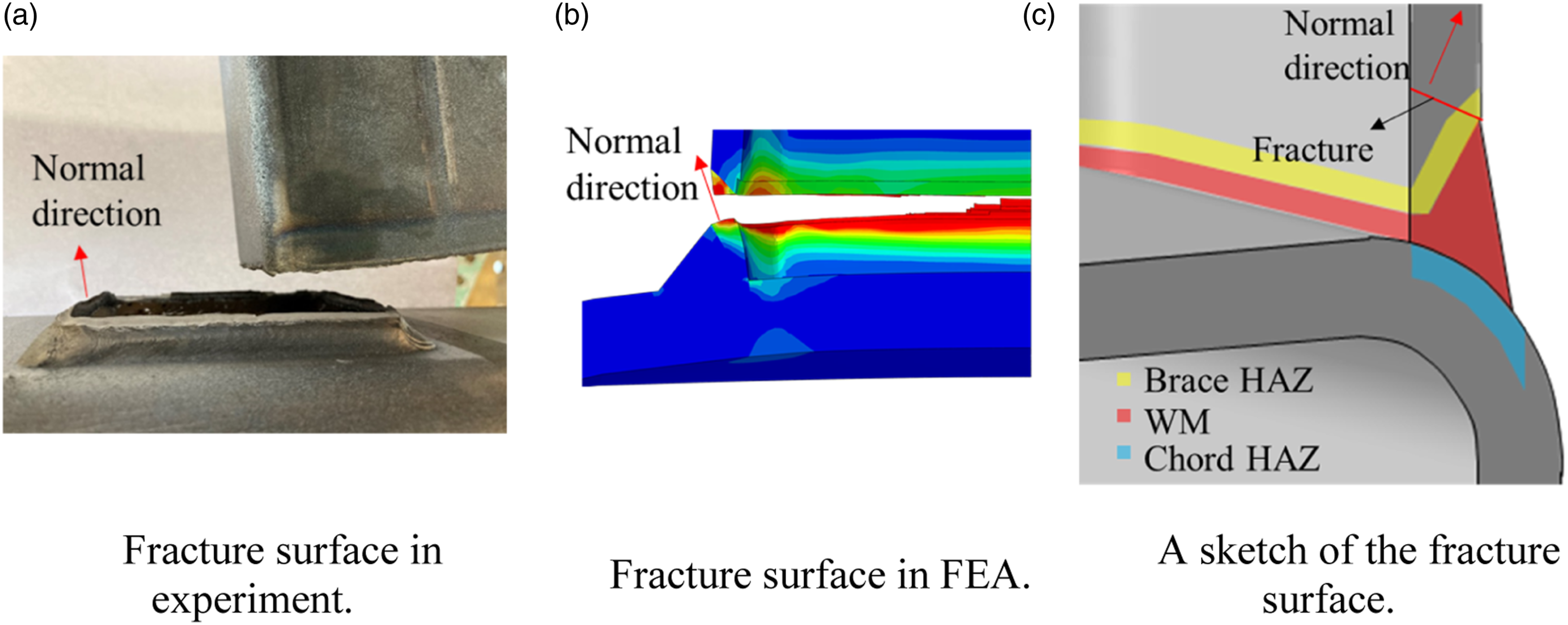
Conclusions and further research
The GTN damage model is implemented into the fracture simulation of welded cold-formed RHS X-joints. Based on the presented results, the following conclusions are drawn: 1. The computational homogenisation is conducted to calibrate the GTN yield-surface parameters (q1 and q2), considering the different combinations of the accumulated initial hardening strain and the VVF ( 2. The undamaged true stress-true strain relationship of the BM is generated using a weighting factor (W) based on the Swift model and the linear model. The weighting factor decreases with the increase of the steel grade, which is around 0.9, 0.7, and 0.1 for S355, S500, and S700 material, respectively. It indicates that the BM undamaged constitutive model gradually transfers from the linear model to the Swift model concerning an ascending steel grade. The HAZ material has a weaker post-necking strain hardening behaviour than BM. The Voce model is suitable for generating the undamaged constitutive model for all HAZ materials. 3. The damage of the element is sensitive to the value of the fracture parameter fc. ff has a minor influence on the failure process. The value of ff, up to 5% larger than fc, is validated in this study. 4. The calibrated GTN damage model for BM and HAZ could effectively predict the fracture-related failure modes: PSF, BF, and CSWF, of welded RHS X-joints in tension, although the material shear failure mechanism is not considered. Comparing the ultimate resistance of the FE models and the experiments (EXP), the FE/EXP ultimate resistance ratio varies from 0.91 to 1.02, with an average 0.98 ratio. 5. Two orientations of the PSF fracture surface are observed in experiments. The FE model successfully predicts the fracture cutting through the profile thickness of the chord, while the fracture propagated below the weld was not accurately predicted. The fractures of BF and CSWF are well predicted. Both BM and HAZ contributed to the fracture of BF. The predicted fracture shape of CSWF may be improved by considering the constitutive model of the corner material in cold-formed RHS tubes. 6. The main limitation of the employed GTN damage model is that the effect of the Lode angle on the material yield and failure criterion is not considered, although the predicted ultimate resistance fits the experiments well. It will be considered in future work and a generic FE model will be validated at various stress states. In addition, a constitutive model for the corner material of cold-formed RHS tubes, including BM and HAZ, should be established based on experimental and numerical studies. Using the validated corner material model, the FE model will be complete to evaluate the effect of high strength and low ductility of corner material on the joint mechanical behaviour.
Footnotes
Declaration of conflicting interests
The author(s) declared no potential conflicts of interest with respect to the research, authorship, and/or publication of this article.
Funding
The author(s) received no financial support for the research, authorship, and/or publication of this article.
Appendix
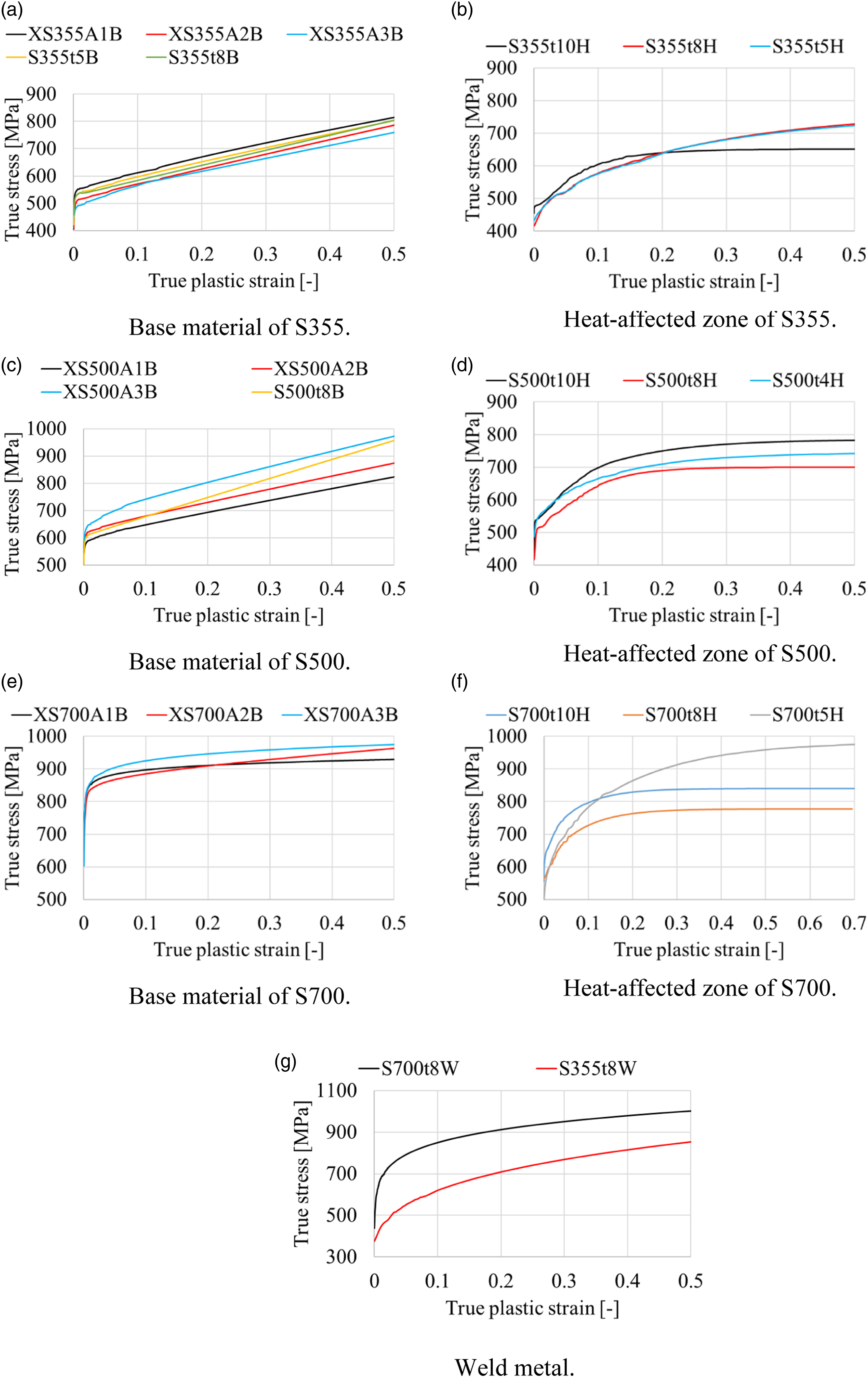
Undamaged true stress-true plastic strain relationships for X-joint simulations.