A novel in-situ temperature measurement method for liquid metal embrittlement cracking analysis

Abstract

Liquid metal embrittlement poses a challenge in resistance spot welding of zinc-coated advanced high-strength steels. Liquid metal embrittlement often leads to surface cracking, which degrades the mechanical properties of the welded joints. Therefore, understanding the liquid metal embrittlement cracking behaviour and developing mitigation strategies are essential. This study proposes the implementation of an infrared camera for in-situ temperature measurement during welding. Given the substantial variation in surface emissivity during resistance spot welding, a temperature correction model is necessary at critical temperatures associated with liquid metal embrittlement onset. This study proposes a temperature correction model that achieves an 85% improvement in accuracy with a 20 °C error. The model is tailored for quantitative analysis of liquid metal embrittlement cracking, utilising the Boltzmann sigmoidal and BiDoesResp functions.

Introduction

Considering the increasing urgency of climate change, it is crucial to focus on lightweight body-in-white (BIW) structures in the automotive industry without compromising their strength while maintaining passenger safety. ¹ A cost-effective option for simultaneously achieving strength and weight reduction is the increased use of third-generation advanced-high-strength steel (3G-AHSS) due to its superior properties compared to previous generations of advanced high-strength steel (AHSS).^2,3 In practice, a zinc-based coating is typically applied to the 3G-AHSS substrate to enhance the corrosion resistance of the BIW materials. This zinc coating functions both as a sacrificial anode and a physical barrier against corrosive elements. ⁴

Although the use of 3G-AHSS provides an excellent weight-saving opportunity, these steels must be joined to form the BIW. Joining the 3G-AHSS typically involves resistance spot welding (RSW) due to high productivity, automation capability, and the fast-paced nature of the process. ⁵ However, when 3G-AHSS is subjected to RSW, a cracking phenomenon known as liquid metal embrittlement (LME) ⁶ may occur on the weld joint surface, particularly around the electrode imprint area. These cracks are caused by molten metal penetrating the solid grain boundaries of the base material, which can reduce ductility and may lead to brittle failure of the grain boundary under stress. In the automotive industry, controlling LME cracks is crucial, as their presence has been linked to premature failure under conventional loading conditions such as shear or tensile loading.^7,8

Numerous studies have been conducted to understand the LME cracking behavior during RSW.^9–11 However, the complex thermal-mechanical history of the RSW process poses significant research challenges. While Gleeble thermo-mechanical simulation has been widely used to study LME mechanism, ¹² the Gleeble system is unable to replicate the exact thermal cycle of the RSW process. ¹⁰ Alternatively, the half-sectioned RSW (H-RSW) procedure is shown to be a better option for simulating the thermal cycle of the RSW process. ¹³ H-RSW enables in-situ temperature monitoring using an infrared (IR) camera.

IR cameras are classified as mono-colour (single wavelength) or two-colour (dual wavelength) systems. While two-colour cameras provide emissivity-independent temperature measurements, they require complex calibration and are less common. ¹⁴ Mono-colour cameras are widely used but rely on an assumed emissivity, which varies with temperature, phase and oxidation, leading to inaccuracies. For instance, Makwana et al. ¹⁴ showed that mono-colour IR measurements during gas metal arc brazing deviated from thermocouple measurements, whereas two-colour cameras achieved close agreement. These studies highlight that while mono-colour systems are practical, emissivity dependence introduces uncertainty, necessitating additional calibration for materials like 3G-AHSS, as investigated in this study, especially for in-situ H-RSW temperature monitoring across the 400 °C–900 °C range relevant to LME cracking.

This study proposes an IR camera calibration method for accurate local temperature measurement during the H-RSW procedure. A Gleeble thermo-mechanical simulator was used to validate the temperature measurements from the IR camera with varying emissivity values. The synchronisation between temperature readouts from the IR camera and the thermocouples led to the development of a temperature correction model that can be directly applied during the thermography of H-RSW. Results indicated that the emissivity values were a function of temperature due to oxidation growth behavior at different temperatures. The developed temperature prediction model enables precise temperature measurement near LME cracks, which is valuable for future H-RSW experiments that aim to mitigate the LME phenomenon by better understanding its formation and propagation mechanisms.

Experimental methodologies

Materials

A 1.6 mm thick galvanised (GI) coated 3G-AHSS with an ultimate tensile strength (UTS) of 980 MPa was used in this study. The as-received microstructure consisted of a combination of ferrite, bainite and tempered martensite as shown in the scanning electron micrograph in Figure 1(a). The chemical composition and the carbon equivalent of the investigated 3G-AHSS are listed in Figure 1(b). The carbon equivalent of the material was calculated using the formula proposed by Yurioka et al. ¹⁵

Figure 1.

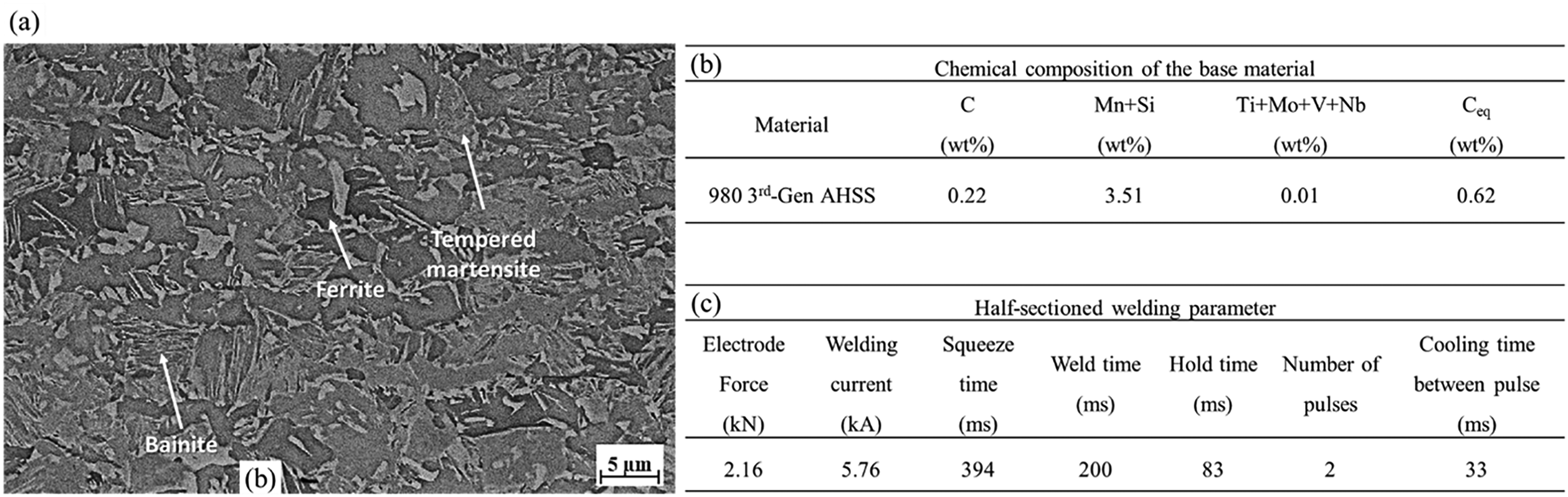
(a) Microstructure of base-metal (3G-AHSS) obtained from a FE-SEM; (b) the chemical composition and carbon equivalent of the investigated material; and (c) half-sectioned welding parameters used in this study.

H-RSW and gleeble experiments

H-RSW was performed using a medium frequency direct current Honda R-2000ic robotic spot welder equipped with an industrial C-type welding gun and a Bosch Rexroth controller. The H-RSW process configuration consists of a pair of electrodes with half-sectioned tip faces, aligned with the edges of the stacked steel sheets. Two similar 25 mm × 25 mm coupons of the 3G-AHSS were used for the H-RSW configuration. The welding force and current used for the H-RSW were less than what would have been used to weld a conventional RSW joint. ¹⁶ The alteration of the H-RSW parameters compared to the RSW was to account for the reduced electrode face area. The methodology for selecting the welding parameters for the H-RSW is outlined in Figure 1(c). Additional detailed information about the H-RSW is described in a previous work. ¹³

An M350 IR camera, manufactured by TELOPS, and a Mini UX100 HS camera by FASTCAM were used for in-situ monitoring of the H-RSW process. The IR camera is equipped with a 50 mm lens and has a spectral range of 1.2–7 μm. The valid temperature range of the utilised lens was from 233 °C to 1500 °C. Both cameras were synchronised using a bayonet Neil-Concelman (BNC) cable. The frame rate for both cameras was set at 1000 fps, with resolutions of 1280 × 1024 for the HS camera and 460 × 124 for the IR camera. Reveal IR software, supplied by the manufacturer, includes an emissivity customisation function that allows the users to adjust a specific emissivity value for an objective material. The default emissivity value in the software is set to 1.00. However, the emissivity was selected to closely match the temperature reading by the thermocouple, as will be discussed in the ‘Results and discussion’ section.

For temperature correction of the IR camera, a Gleeble 3500 thermomechanical simulator was used. The temperature correction process involved matching the temperature readings from the thermocouples with the outputs of the IR camera. Custom sub-sized tensile specimens, with dimensions outlined in Figure 2(a), were used for the Gleeble experiments. Given that emissivity is affected by the surface condition of the specimens,^16,17 consistent surface preparation was maintained for both the welded samples and those used for Gleeble. The edges of the Gleeble and H-RSW coupons were polished using 180-grit silicon carbide sandpaper. Surface profiling was performed using a Keyence VK-200 series optical microscope to ensure that the surface roughness of the Gleeble and H-RSW specimens was comparable, as demonstrated in Figure 2(b). The average surface roughness values for the Gleeble and H-RSW specimens were similar, at 1.93 and 1.83 μm, respectively. Two specimens with different time intervals between sample preparation and the Gleeble test were prepared to investigate the effect of the initial surface condition. The specimen was prepared 7 days before the experiment. Then, the sample was exposed to air, referred to as the 7-day sample. The 1-day sample refers to a specimen with a time interval of one day between sample preparation and Gleeble experiments.

Figure 2.

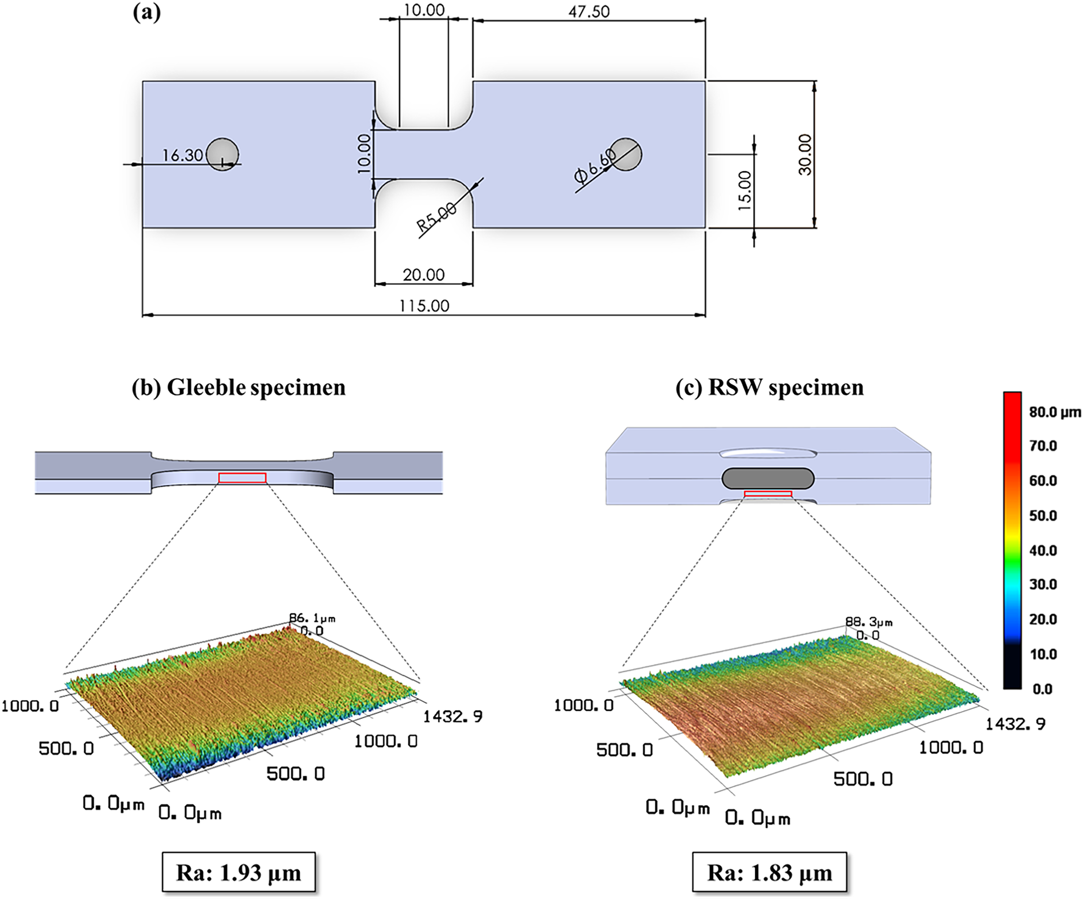
(a) Dimensions of the sub-sized Gleeble coupon; average surface roughness of (b) Gleeble and (c) half-sectioned resistance spot welding (H-RSW) specimen.

Figure 3 illustrates the calibration setup for the IR camera and the configuration of the Gleeble specimen, which has two sets of thermocouples attached. To enhance the weldability of the thermocouples to the specimen, the Zn coating was initially removed from the designated area. The IR camera was positioned to focus on the edge of the specimen, identified as the area of interest (AOI) in Figure 3. Two sets of thermocouples were attached to the Gleeble specimen: Thermocouple 1 (TC1), located at the centre of the gauge, is utilised to regulate the temperature in the Gleeble system, whereas Thermocouple 2 (TC2) was positioned near the edge to compare temperatures between the IR camera and the thermocouple.

Figure 3.

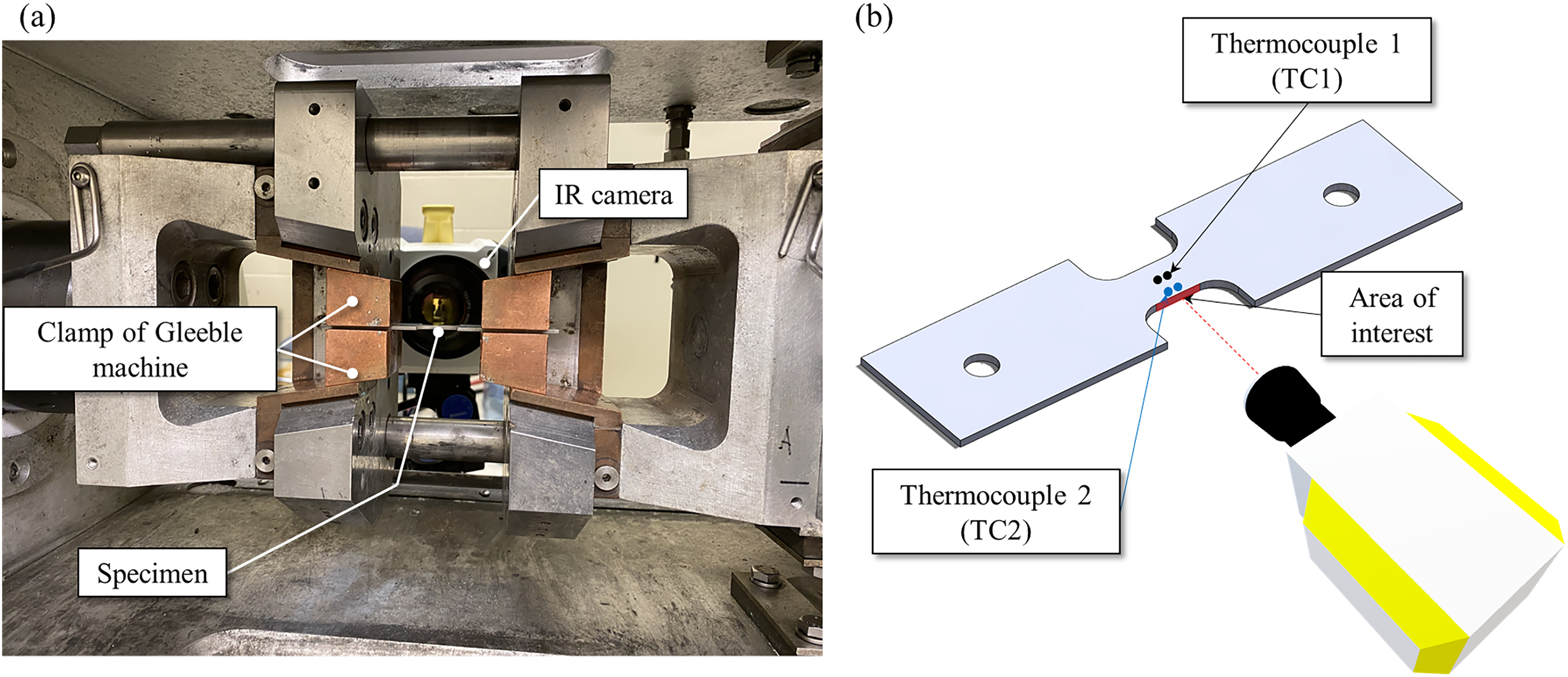
(a) Infrared (IR) camera calibration setup and (b) schematic of the configuration for a Gleeble specimen with attached thermocouples.

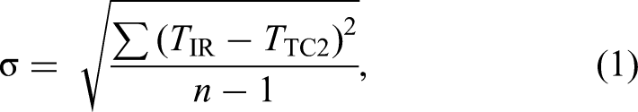
The error range between the IR camera data and the thermocouple can be calculated using equation (1) to quantitatively validate the output of the IR camera compared to the reference temperature.

$$\sigma =\sqrt{{\displaystyle \frac{\sum {(T_{\mathrm{IR}}-T_{\mathrm{TC}2})}^2}{n-1}}},$$

(1)

where T_IR is the temperature measured by the IR camera at the TC2 junction point, T_TC2 is the temperature measured from the TC2, and n is the number of data points. A minimum of five data points were collected at each sub-region, as described in the dynamic emissivity range. To ensure consistency across different emissivity values, the data points were selected such that the temperature measurements for each emissivity were taken simultaneously.

To conduct metallographic observations, specimens for base metal were hot-mounted in electrically conductive resin and polished using conventional metallographic procedures. They were then etched with a 2% nital solution for scanning electron microscopy (SEM) examination. SEM was performed using a Zeiss LEO 1530 Field emission SEM. X-ray diffraction (XRD) was conducted to examine the oxidation on the specimen's surface using Bruker D8-discover with Cuk_α radiation and VANTEC500 detector.

Results and discussion

Dynamic emissivity range

The temperature profile obtained from the IR camera and TC2 during the Gleeble thermal-mechanical simulation with a heating rate of 1000 °C/s is shown in Figure 4(a). The set temperature was 1300 °C with a hold time of 4 s (red TC2 curve in Figure 4(a)). Readouts from the IR camera in Figure 4(a) have been plotted for three different emissivity values (ε = 0.35, 0.66 and 1.00). A sudden shift in the increasing trend of the temperature was noted from the IR camera readouts, between 776 °C and 804 °C. Interestingly, this sudden transition in temperature behaviour was not observed in the readouts from the TC2. The temperature shift phenomenon has also been observed in the literature for the heat treatment and electrical seam welding of low-carbon steel. ¹⁶ Changes to the specimen surface condition (such as rapid oxidation) have been associated with the root cause of such temperature anomalies. Henceforth, this temperature shift phenomenon is referred to as the dynamic emissivity range. Figure 4(b) shows an enlarged view of the near-dynamic emissivity region.

Figure 4.

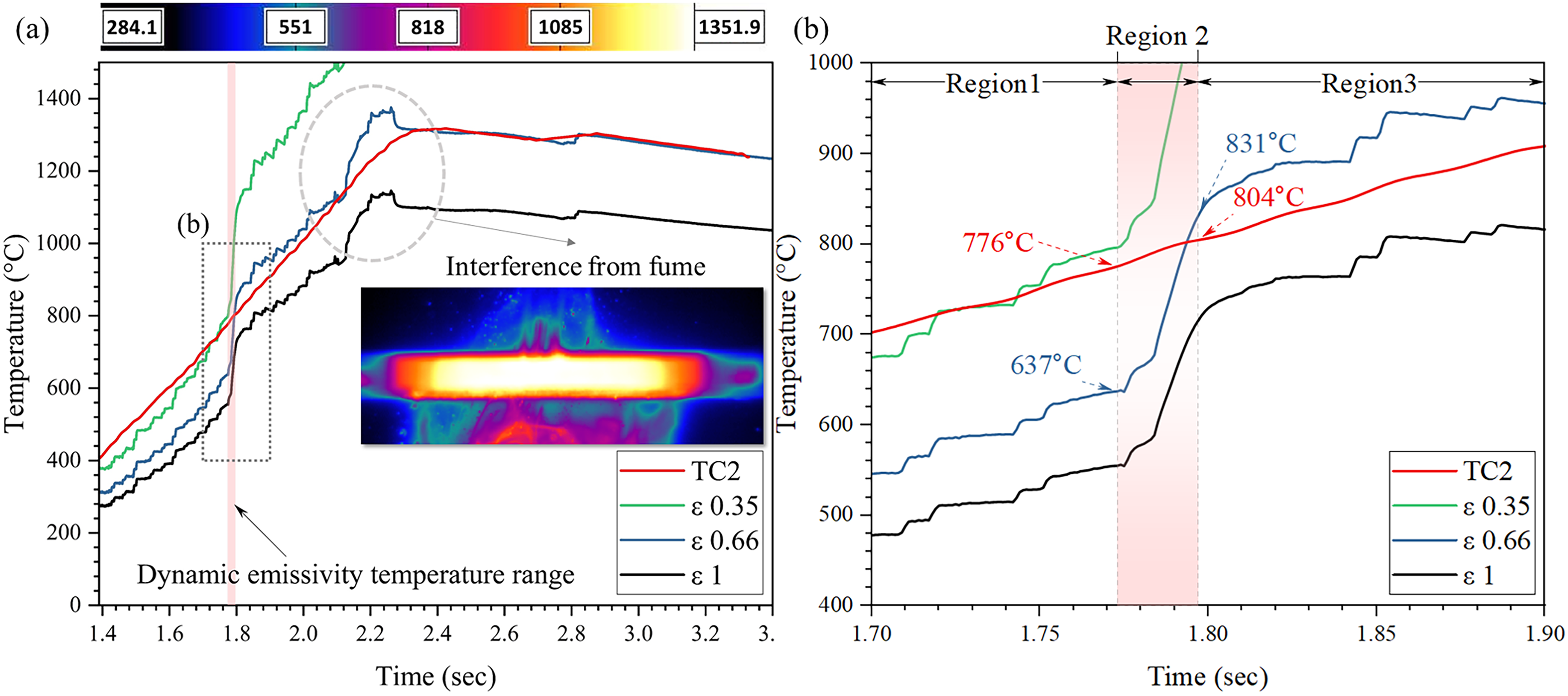
(a) Temperature profile from the IR camera with various emissivity values compared to TC2 and (b) an enlarged view in the dynamic emissivity range (776 °C–804 °C).

All readouts from the IR camera with three different emissivity levels (ε = 0.35, 0.66 and 1.00) were compared against the TC2 measurements (reference temperature in AOI) (Figure 3). It is noted that ε = 1.00 was the default emissivity value in Reveal IR post-processing software, while ε = 0.35 and 0.66 were selected due to their best agreement with the reference temperature TC2 (Figure 4(a)). More specifically, ε = 0.35 matches best with the TC2 measurements before the dynamic emissivity region, whereas ε = 0.66 matches the TC2 data after the dynamic emissivity transition.

The temperature profile measured by the IR camera can be subdivided into three regions based on their emissivity characteristics. Region 1 is classified as the temperature range before the dynamic emissivity phenomenon (below 776 °C). Region 2 is identified by a narrow temperature spectrum (between 776 °C and 804 °C). In this region, the IR temperature readings exhibit a distinct change in behaviour, with the temperature measured by the IR camera increasing faster than the temperature measured by the TC2, as shown in Figure 4(b), indicating a continuous alteration in emissivity value within the temperature range associated with Region 2. Lastly, Region 3 is referred to as the temperatures above 804 °C. The error range, as calculated using equation (1), in Region 1 was determined to be 50.47 °C, 155.13 °C and 215.61 °C, with an emissivity of 0.35. 0.66 and 1.00, respectively. For Region 2, the error range values were measured to be 136.95 °C, 111.25 °C and 205.95 °C for emissivity values of 0.35, 0.66 and 1.00, respectively. Lastly, for Region 3, the error ranges were measured at 509.27 °C, 5.11 °C and 237.99 °C for the selected emissivity values. At the beginning of Region 3, overshooting was observed in the IR camera output. The overestimation of the temperatures in Region 3 compared to the data from TC2 is due to the interference of welding fumes with the IR camera, as highlighted in Figure 4(a). These fumes are associated with the vaporisation of the Zn coating during the heating process on the opposing side of the TC2 attachment, where the Zn coating was not removed. However, the temperature measurement by the IR camera becomes stable after surpassing the Zn vaporisation temperature (∼907 °C). It is noted that the disturbed temperature measurements due to welding fumes were excluded from the error range calculation in Region 3.

The existence of the dynamic emissivity range is problematic for LME analysis as its temperature range coincides with the LME critical temperature (700 °C–900 °C). ¹⁷ The following sub-section (effect of surface condition on IR temperature measurements) clarifies how sample surface conditions affect emissivity values. Temperature correction method for the IR camera, on the other hand, elaborates on the methodology utilised to obtain the correct emissivity value at LME-critical temperatures, as well as the calibration of a model that scales the IR readouts to the correct reference temperature from TC2.

Effect of surface condition on IR temperature measurements

Surface condition significantly influences specimen emissivity, as established in the dynamic emissivity range. Iron oxides – including wüstite (FeO), magnetite (Fe₃O₄) and hematite (Fe₂O₃) – form through diffusion-controlled mechanisms exhibiting parabolic growth kinetics. ¹⁶ As the oxide layer thickness increases, these compounds alter emissivity through interferential effects on thermal radiation, with growth characteristics varying according to the treatment conditions. ¹⁶

To understand the influence of initial surface roughness and progressive oxidation on emissivity measurements during the Gleeble tests, samples were tested at two distinct time intervals following the Sic grit 180 surface preparation. The first set of samples was tested 1 day after grinding, and the second set of samples was tested 7 days after the surface grinding. All process parameters remained constant, isolating surface condition as the sole variable. Despite maintaining a fixed Gleeble temperature of 700 °C, the specimens exhibited distinctly different matched emissivity values – 0.35 for the 1-day specimen and 0.66 for the 7-day specimen, as shown in Figure 5(a) and (b).

Figure 5.

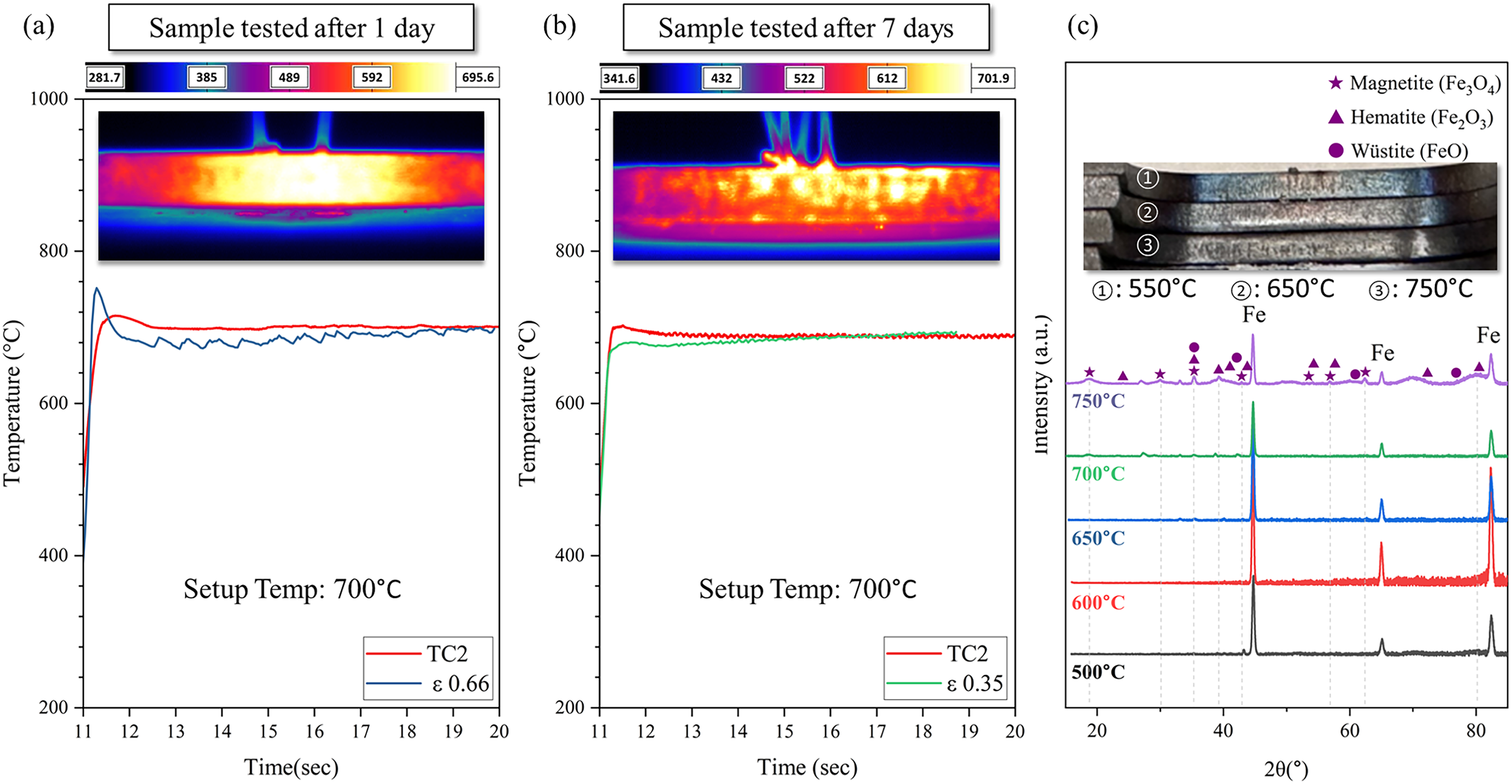
Temperature measurements from the IR camera and TC2 with samples tested after (a) 1 day and (b) 7 days. (c) XRD results of specimens heated to temperatures between 500 °C and 750 °C and optical image of the specimens’ surface after the Gleeble test.

XRD analysis was performed on specimens that were prepared 1 day before the Gleeble test and heated between 500 °C and 750 °C to elucidate the underlying mechanisms responsible for variations in emissivity. Peak identification utilised International Centre for Diffraction Data (ICDD) reference codes: 00-033-0664 (hematite), 00-006-0615 (wüstite) and 19-0629 (magnetite). ¹⁷ The analysis revealed negligible wüstite formation across all tested specimens. However, magnetite peaks became evident at 700 °C, with both peak intensity and number of aligned peaks increasing progressively with temperature. Specimens heated to 750 °C exhibited pronounced formation of a magnetite layer, accompanied by corresponding decreases in iron peak intensity. Optical images of the samples corroborated these findings, showing temperature-dependent surface colour variations attributable to oxide formation (insets of Figure 5(c)).

The combined XRD and optical evidence confirm that magnetite formation drives the dynamic emissivity behaviour observed in the critical temperature range of the investigated materials. This mechanism explains the thermal mapping discrepancies between specimen types: 1-day samples exhibit non-uniform temperature distributions due to incipient magnetite formation at discrete locations, whereas 7-day samples display uniform distributions owing to the complete development of an oxide layer. Consequently, precise IR temperature monitoring requires standardised specimen preparation protocols with controlled time intervals between surface preparation and testing. Based on these findings, all subsequent Gleeble specimens were prepared one day prior to experimentation to ensure measurement consistency.

Temperature correction method for the IR camera

Since the dynamic emissivity region overlaps with the critical temperature range for the LME cracking, developing temperature correction methods for this region is necessary for quantitative analysis of LME cracks. Nevertheless, temperature correction for Region 2 is challenging due to the emissivity value continuously changing with increasing temperature.

To characterise the temperature-dependent emissivity behavior, 25 Gleeble experiments were conducted across various temperature ranges to establish the relationship between emissivity and temperature. The experimental data exhibited distinct upper and lower bounds with a monotonic increasing trend, indicating that a sigmoidal modeling approach would provide optimal fitting characteristics. As shown in Figure 6(a), applying the sigmoidal model yielded an R² value of 0.95, indicating that the model accurately predicts the emissivity value. Such temperature-dependent emissivity behaviour and the emissivity prediction curve using a sigmoidal function have also been observed in the study by Santos de Deus and co-authors. ¹⁸ The validated model definitively establishes that the dynamic emissivity region spans 700 °C–900 °C, with emissivity values ranging from 0.35 to 0.66.

Figure 6.

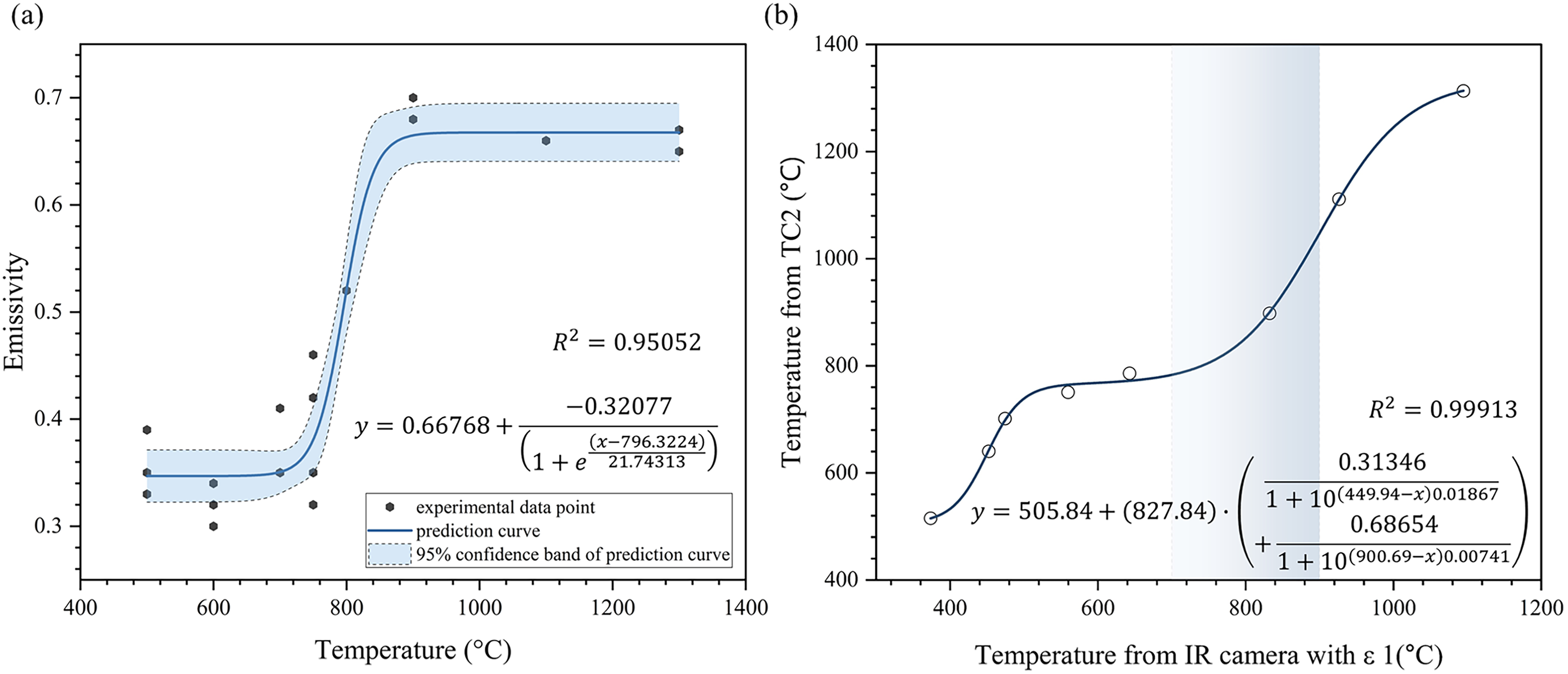
(a) Emissivity prediction curve by Boltzmann sigmoidal model over temperature with 95% confidence band and (b) the temperature correction curve for the infrared (IR) camera.

The physical mechanism underlying this behavior involves the initiation of magnetite formation at 700 °C, followed by continuous oxide layer growth until 900 °C, where the saturation thickness is achieved. Beyond 900 °C, emissivity remains constant due to the stabilised oxide layer structure. This temperature-dependent emissivity variation aligns well with established literature findings.^16,18

Quantitative LME crack analysis requires temperature measurements spanning a broad thermal range that encompasses both static and dynamic emissivity regions (Regions 1–3, as described in the dynamic emissivity range). Since the Reveal IR software lacks integrated dynamic emissivity functionality, a dedicated temperature scaling methodology was developed to convert IR camera readouts to accurate reference temperatures. Using the comprehensive Gleeble dataset employed for emissivity prediction, the relationship between IR camera measurements (at unity emissivity) and reference temperatures was investigated across multiple experimental conditions. The Biphasic Dose-Response Function (BiDoseResp) model, available in the Originlab^® non-linear regression library, demonstrated an excellent correlation between IR camera outputs and reference temperatures, as illustrated in Figure 6(b). This model provides highly accurate temperature conversion capabilities with defined operational bounds of 506 °C (lower limit) and 1334 °C (upper limit). The following procedure can be applied by combining the emissivity prediction model with the temperature correction model for the dynamic emissivity region.

The combined temperature correction methodology integrates both emissivity prediction and temperature scaling models to enable comprehensive thermal analysis through a systematic implementation procedure that begins with initial temperature acquisition, where temperatures are recorded at the area of interest using IR camera software with a unity emissivity setting. Following this primary calibration step, the BiDoesResp-based temperature correction model is applied to calibrate measured temperatures within the operational bounds of 506 °C–1334 °C. For boundary condition management, temperatures falling outside the model bounds require the application of fixed emissivity values, specifically 0.35 for temperatures below 506 °C and 0.66 for temperatures above 1334 °C.

Temperature correction model validation and its application in LME crack analysis

The temperature correction curve, which scales the temperature measured by the IR camera with an emissivity value of 1.00, was applied to the IR camera readout data used in Figure 4. Since the temperature below 700 °C has a consistent emissivity value, the temperature was measured with an emissivity value of 0.35. The temperature range between 700 °C and 900 °C was the focus of the BiDoesResp model, which was applied to temperature correction for this particular range. For temperatures above 900 °C, the emissivity value of 0.66 was used, as it represents the upper bound of the BiDoesResp model. Figure 7 shows the temperature profile after applying the temperature correction model, compared to the profile without calibration and the reference temperature. The error range, calculated using equation (1), was 47 °C for Region 1, 23 °C for Region 2 and 5 °C for Region 3. It is essential to note that the temperature correction results in a substantial reduction in error in Region 2, compared to the mean error of 151 °C obtained from three emissivity values (0.35, 0.66 and 1.00), which represents the case without calibration.

Figure 7.

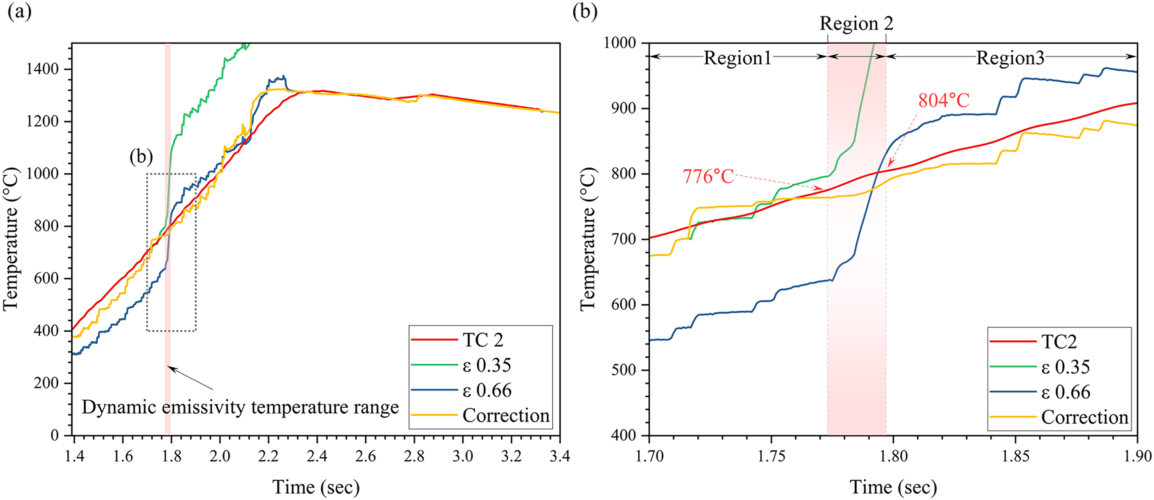
(a) Temperature profile from the infrared (IR) camera with a range of emissivity values, temperature correction method, and (b) enlarged view at dynamic emissivity range.

The developed combined temperature correction model is helpful for the quantitative analysis of LME cracking during the H-RSW process. For example, in-situ temperature monitoring at the exact location of LME crack initiation has not yet been achieved; however, the following approach enables a quantitative analysis of the LME crack. In a synchronised camera system, the HS camera is used to precisely determine the LME crack location, as shown in Figure 8(a). The LME crack location can be defined in the thermal map using the HS camera information. Thus, the temperature history at the LME crack initiation point (A) and 240 μm away from the crack location (B) can be obtained using the IR camera to compare the temperature changes with respect to welding time (Figure 8(c)). Furthermore, since the HS camera can define the welding time of LME crack initiation, the temperature at which LME crack initiation occurs can be specified as 732 °C. The thermal profile at points A and B with respect to welding time can then be compared, as shown in Figure 8(b).

Figure 8.

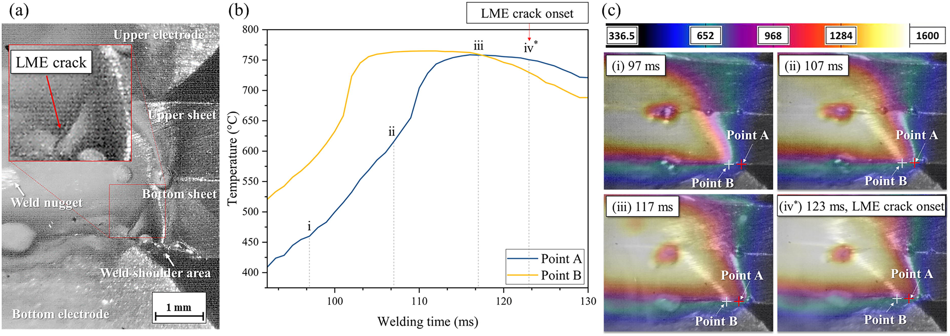
(a) An example of high-speed camera footage showing the liquid metal embrittlement (LME) crack at the shoulder region of the bottom sheet, (b) the thermal history at the LME crack location and (c) a thermal map highlighted in the temperature profile.

The temperature history of both points A and B appears similar, as shown in Figure 8(b): a sharp temperature rise, followed by a plateau at a specific temperature, and then a subsequent decrease. The two temperature profiles intersect at a particular point (welding time of 117 ms), indicating the onset of temperature decrease at point B. This decrease is attributed to the mechanical collapse between the electrode and the substrate, which dissipates surface heat to the electrode as the electrode acts as a heat sink. Following the intersection point, the temperature difference between points A and B progressively increases, eventually leading to crack formation at a welding time of 123 ms. Such behaviour is similar to the finite elements modeling (FEM) simulation results reported by DiGiovanni et al. ¹⁹ in which abrupt temperature gradients caused by electrode collapse generate thermal stress. The thermal map with four different welding times of 97 ms (i), 107 ms (ii), 117 ms (iii) and 123 ms (iv*), well describes the electrode-to-substrate contact behavior and the corresponding temperature distribution. At the welding time of 97 ms (i), the temperature at points A and B increases with increasing welding time. During the welding time of 107 ms (ii), the temperature at point A continues to increase while point B enters the plateau temperature region. Point B came into contact with the electrode, decreasing the temperature at the point, while the temperature at point A remained in the plateau region. As a result of heat dissipation toward the electrode at point B, the temperature gap between points A and B gradually increased. At the welding time of 123 ms, an LME crack initiation was observed, indicating that the critical tensile stress required for the crack formation was reached at this moment. This suggests that the crack was likely caused by the thermal stress resulting from the temperature difference between the two points. Therefore, the temperature correction method introduced in this study suggests the possibility of conducting a focused quantitative analysis on specific crack formation.

Conclusions

This study developed a novel temperature correction methodology designed to improve the accuracy of IR temperature measurement during LME analysis of 3G-AHSS. The investigation revealed that the formation of iron oxides drives variations in emissivity under elevated temperatures. Through Gleeble experiments, the emissivity behaviour demonstrated excellent correlation with a Boltzmann sigmoidal model (R² = 0.95), establishing the critical emissivity range of 0.35–0.66. The integrated temperature correction framework combines an emissivity prediction model with a BiDoesResp-based temperature scaling model operating within bounds of 506 °C–1334 °C. The correction model reduced measurement errors in the critical dynamic emissivity region from 151 °C to 23 °C, representing an 85% improvement in accuracy.

Validation through synchronised high-speed and infrared camera systems revealed the critical temperature of 732 °C for LME crack initiation. The analysis demonstrated that electrode collapse during welding creates progressive temperature gradients between crack sites and adjacent regions, with the temperature differential increasing until reaching the threshold for crack formation. This temperature correction methodology provides new insights into the quantitative analysis of the thermal-mechanical mechanisms governing LME formation and propagation in AHSS welding applications.