
Abstract
As policy makers require more rigorous assessments for the strength of evidence in Theory-Based evaluations, Bayesian logic is attracting increasing interest; however, the estimation of probabilities that this logic (almost) inevitably requires presents challenges. Probabilities can be estimated on the basis of empirical frequencies, but such data are often unavailable for most mechanisms that are objects of evaluation. Subjective probability elicitation techniques are well established in other fields and potentially applicable, but they present potential challenges and might not always be feasible. We introduce the community to a third way: simulated probabilities. We provide proof of concept that simulation can be used to estimate probabilities in diagnostic evaluation and illustrate our case with an application to health policy.
Introduction
Trusting evaluation evidence is crucial if policy decisions are to be grounded on evaluation findings; whether the latter are credible or not has very practical implications for the decision-making process. While policy makers and analysts are developing an increasing interest in Theory-Based Evaluation, the discussion around what constitutes credible evidence in this domain is somewhat weaker and less advanced than agreed corresponding protocols for quantitative methods; this is particularly true when claims are causal.
Establishing causal connections is often challenging in social systems, due to difficulties in disentangling interdependencies, and in isolating causes from particular contexts and confounding factors (Byrne and Callaghan, 2013). This is exacerbated when time is one of these factors because of the additional difficulty in capturing changing systems and their often-emergent dynamics. This is a problem for evaluation, in particular impact evaluation, as it is essential to show that a particular (set of) intervention(s) has brought about, or caused, a particular (set of) outcomes.
Evaluation has developed a range of methods to draw out causal relationships that are distinct from established tools like randomised controlled trials (RCTs) (Befani and O’Donnell, 2016; Stern et al., 2012), which is often seen as the gold standard but requires that the environment be controlled. Diagnostic Theory-Based Evaluation, which applies Bayesian Updating to Theory-Based Evaluation, has been proposed as a promising methodology to account for the uncertainty inherent in testing causal theories or mechanisms (Befani, 2020a). Historically, when Bayesian principles have been applied to theory-based evaluation, various labels have been used: Bayesian Process Tracing (Fairfield and Charman, 2017), Process Tracing with Bayesian Updating (Befani et al., 2016), and Contribution Tracing (Befani and Stedman-Bryce, 2017).
What these methods have in common (which are the basic ingredients of Diagnostic Evaluation) is that they link empirical data to theoretical propositions with a three-step diagnostic approach:
Formulating a (set of) claim(s) describing the contribution that an intervention and/or other factors have made to an outcome;
Designing data collection with the aim of identifying conclusive evidence in support of or against the contribution claim(s);
Formally estimating the ‘strength’ or probative value of single observations, as well as evidence ‘packages’, and consequently updating (prior) confidence in the claim(s) on the basis of the evidence (obtaining the ‘posterior’ confidence” according to the Bayes formula).
Step 1 is often grounded on a narrative analysis of the case from which causal claims leading to a particular outcome are extracted. Step 2 establishes what evidence is likely to support or reject the claims, painting a rough, intuitive picture of the strength and direction of the various observations (and of them taken as a whole). Step 3 analyses the probative value of observations for the different hypotheses in more detail, formalising probabilities and using the Bayes formula for an accurate estimation of the posterior confidence. 1
The advantage of Bayesian Updating (BU) is that applying the Bayes rule to assess the contribution of evidence improves the transparency/replicability of the process and hence the credibility and reliability of a theory. The disadvantage of a Bayesian formalisation is that it requires the estimation of probability values. While a user-friendly alternative to this requirement has been proposed (whereby qualitative estimates are translated into numerical ranges via rubrics) (Befani, 2020b), the estimation of probabilities, either direct or indirect, is still a central feature of BU.
There are two main approaches to estimate these probabilities: empirical frequencies and/or expert judgement. Frequencies are often unavailable or unobtainable, in particular in evaluation research where single case causal narratives are demanded. As for expert opinion, it might be hard in some cases to estimate the empirical consequences of various theories being true or false, even with the best resources; other times it might simply be unfeasible or outside available evaluation budgets.
This paper proposes as a ‘third way’: the use of simulation methods to generate in silico frequencies for particular pieces of evidence in Diagnostic Evaluation, or Bayesian Updating applied to Theory-Based Evaluation. For this, we use a proof-of-concept example of an influenza epidemic, modelling different levels of efficacy of mitigation strategies. By exploring the plausible level of epidemic spread in a population, given particular mitigation strategies, we generate likelihoods that a particular empirically observed level of spread was caused by that kind of mitigation strategy.
The paper is structured as follows. Section ‘Bayesian Updating in diagnostic evaluation’ discusses Bayesian Updating and Diagnostic Evaluation in more detail. Section ‘Generating probability distributions with models’ outlines how models can be used to generate simulated probabilities and describes the simulation model of behaviour during an epidemic that we are using as an example. Section ‘Estimating Bayes probabilities using the TELL ME Model’ provides a step by step walk through using the example model results to update the Bayes formula probabilities. Section ‘Conclusion’ concludes and discusses limitations and possibilities of this proof-of-concept application for real life evaluation.
Bayesian Updating in diagnostic evaluation
Bayesian Updating (BU) is a systematic application of the Bayes formula to learn from empirical observations (e.g. Howson and Urbach, 2006). Its purpose is to update our confidence that a proposition or statement (including one of causal nature) is true or not true. We represent confidence with a probability (a number between 0 and 1) and distinguish between our level of confidence in the statement before and after observation of evidence (prior and posterior respectively in Bayesian terms).
The process of BU, leading from the prior (pre-observation) to the posterior (post-observation) confidence, is conducted by applying the Bayes formula in its extended version, where P refers to probability, ¬ denotes the logical operator ‘not’, C is a contribution claim and E an empirical observation
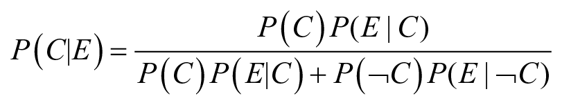
In this equation, P(C) is the probability of the claim before observing the evidence, or prior probability, and P(¬C) is its inverse (the probability of the claim being not true before observing empirical data). P(E|C) is the sensitivity, the probability that the evidence is observed if the causal claim is true (or the true positive rate). Finally, P(E|¬C) is the Type 1 error, the probability that the evidence is observed if the causal claim is false (or false positive rate).
The interpretation of this equation is that the updated probability that the claim C is true after observing evidence E (referred to as posterior probability and denoted P(C|E)) can be calculated once the prior, the sensitivity and the Type I error are known
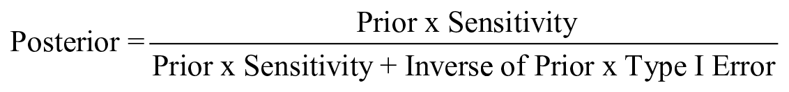
For the purpose of evaluation, BU can be used to understand the value of a piece of evidence in support of or against causal contribution claims. This is usually measured with the Likelihood Ratio or some logarithmic version of it and referred to as ‘probative’ value (i.e. serving as ‘proof’ for the statement). The stronger the evidence, the larger the difference between posterior and prior: or the more the evidence has altered our initial beliefs (see Figure 1). When evidence is strongest, the level of our initial confidence does not matter, and the value of the prior will be dominated by the empirical observation (a.k.a. ‘washing’ of the prior).
The likelihood ratio (LR) = sensitivity/Type I error.
There have been various attempts at using Bayesian Updating with particular evaluation methods:
The Bayes formula is associated with an entire school of probabilistic thinking and its use in evaluation does not have to be associated with specific methods. In its most generalised version, the Bayes formula is applied to any kind of ‘events’ that are hypothesised to exist. For this reason, we explore its potential in relation to Theory-Based Evaluation (TBE) as a whole, rather than to particular TBE formulations like Process Tracing or CA. We use the term ‘Diagnostic Evaluation’ for this generalised approach combining BU and TBE; and this article aims at expanding the range of theories BU can be applied to, to include systems-based evaluation and theories grounded in complex adaptive systems: in particular, the theory of the example we present is formulated as an Agent-Based Model (ABM).
In general, in TBE, we would have a series of claims, which can be competing or complementary. Applying (formal or informal) Bayesian logic, our aim would be to assess our confidence that these claims are true or false. The same empirical observation will usually have a different probative value for different claims, and the same claim is supported to different extents by different observations. That is, the same observation will have different sensitivity and Type I error values against different causal claims. For example, returning three heads on three coin tosses is not very surprising if the coin is believed to be fair, but would be very surprising if the coin is weighted so that heads occurs only 10% of the time. Technically, this means that the Bayes formula values are associated to one claim and one piece of evidence at a time. It also means that, potentially, several values need to be estimated to compare observations and claims, and adjudicate which explanations are best supported empirically.
It becomes crucial to obtain reliable and robust estimates of these values. There are two traditional, well-established strategies that can be used for this purpose: empirical frequencies and subjective estimates (or expert assessments).
When frequencies are available, observations can be used as consecutive empirical inputs leading to inductive inference, that is, each observed white swan supports the claim that all swans are white. Another example is testing the goodness of blood tests as a diagnostic instrument by measuring how many times they correctly identify an underlying disease that is eventually confirmed or ruled out. For example, a blood test can be sensitive but not specific if it is good at ruling out a condition (by showing up as negative when the condition is absent) but not good at confirming its presence (when showing up as positive when the condition is present); or it can be specific but not sensitive if it is good at confirming a condition (showing up as positive when the condition is present) but not good at ruling it out (showing up as negative when it is absent). In the first case, the probability of observing a positive value of the test if the condition is present is high, but the probability of observing the same value if the condition is absent is not low. In the second case, the probability of observing a positive value of the test if the condition is absent is low, but the probability of observing the same value if the condition is present is not high.
When empirical frequencies are not available, subjective probabilities can be elicited from different sources such as stakeholders. There are well-known elicitation procedures in existence such as the Sheffield method (a.k.a. SHELF) (Oakley and O’Hagan, 2016), Cooke’s method (Cooke, 1991), and the Delphi method (EFSA, 2014). These mainly differ on the level and forms of interactions among the experts involved. These methods also acknowledge and try to prevent the typical biases involved in eliciting probabilities: overconfidence, anchoring and adjustment, availability, and representativeness (Block and Harper, 1991).
However, it might not always be possible in evaluations to raise the additional resources needed to estimate probabilities subjectively, and particularly when simulation models are already available for particular aspects of a TBE, using them to update confidence in contribution claims seems a natural and cost-effective option. The next section will discuss the generation of probability distributions through computer-based simulation, and explain why we chose an ABM.
Generating probability distributions with models
Consider further the example of tossing a possibly biased coin three times. The probability of different outcomes is summarised by the binomial distribution, which calculates the number of successes in a sequence of trials with a fixed probability of success in each trial. In this case, success would represent the coin showing heads, and the relevant fixed probability is the bias in the coin. While the probability distribution can be derived analytically in this simple case for any assumed value of the bias, the distribution could also be estimated by simulation. To estimate the outcome distribution of three coin tosses for both 10% and 50% probability of heads, multiple simulations of three tosses would be required for each hypothesis. For example, a physical process to simulate both 10% and 50% bias coin tosses could use a 10 sided fair die. Rolling a ‘1’ would represent the coin coming up head for the 10% head hypothesis, rolling any odd number, that is, 1, 3, 5, 7, and 9, would represent the coin coming up head for the 50% hypothesis. Each set of three die rolls would represent a simulated outcome of three coin tosses. Computationally, simulation outcomes could be generated by drawing from a uniform random number generator instead of rolling a die. This example is clearly very simple (and overly laboured), but generating a distribution of outcomes for diagnostic evaluation would use the same approach; the difference is in the complexity of the process being represented in the simulation model. For more complex processes, an analytical approach is not viable, but the probabilities can still be estimated with computer-based simulations.
There are many methods available to model aspects of systems to be evaluated, each of which makes different assumptions about the process being represented (Badham, 2010; Kelly et al., 2013; Page, 2018). One key difference between methods is whether they model system entities such as people or firms individually or in aggregate. For example, system dynamics represents systems as stocks (quantities of an entity) and flows between stocks (Sterman 2000). This is ideal where the entities are homogeneous, such as water or money, or where entities can be represented effectively by their average characteristics. However, with the focus on average behaviour, it is unusual to include randomness in system dynamics models (Sterman, 2000). In contrast, randomness is inherent in many methods that represent individual entities, including agent-based modelling, discrete event simulation and microsimulation. For example, discrete event simulation is typically used to model systems with queues such as customer service centres or factory production lines (Banks et al., 1996). The variation in arrival times or process times is important in creating bottlenecks or idle periods and simulating each entity individually allows such system behaviours to be created in the model. Microsimulations model transitions of individuals from one state to another within a particular time frame (e.g. dying, becoming unemployed within the next year) explicitly with probabilities to, for example, estimate future pension or welfare costs (e.g. Mitton et al., 2000). Agent-based modelling uses stochastic elements in various ways, particularly to model agent decision making processes taking into account the characteristics and situation of the agent (e.g. Gilbert, 2008).
As randomness is required to generate different outcomes within a set of simulations, our demonstration model uses an individual based method, in this case agent-based modelling. Agent-based modelling ‘is a computational method that enables a researcher to create, analyse, and experiment with models composed of agents that interact within an environment’ (Gilbert, 2008: 2). ABMs function as a virtual laboratory for repeated experimentation. Letting individual agents interact with each other allows ABM to simulate macro phenomena resulting from aggregation of the individual interactions, for example, the level of overall segregation resulting from tolerance levels of mixed neighbourhoods (Schelling, 1971), or the market price from locally traded good (Epstein and Axtell, 1996).
ABM can be used to better understand complex systems that involve emergent phenomena, feedback loops, tipping points and path dependencies, which are often at the heart of the problem of attributing causality in real-world scenarios (Edmonds et al., 2019). The way ABM does this is by representing the mechanisms which generate those phenomena based on our best available understanding of the theory. By experimenting in silico with different parameter settings, e.g. tolerance levels, levels of supply of a good, the user can develop an understanding of the link between initial settings and macro outcomes, and therefore of causal narratives and their plausibility. Exploring the parameter space allows us to reason backwards, from an outcome to the set of input parameters that most likely lead to this particular outcome. This paper advocates an application of ABM that is at the same time
The TELL ME ABM
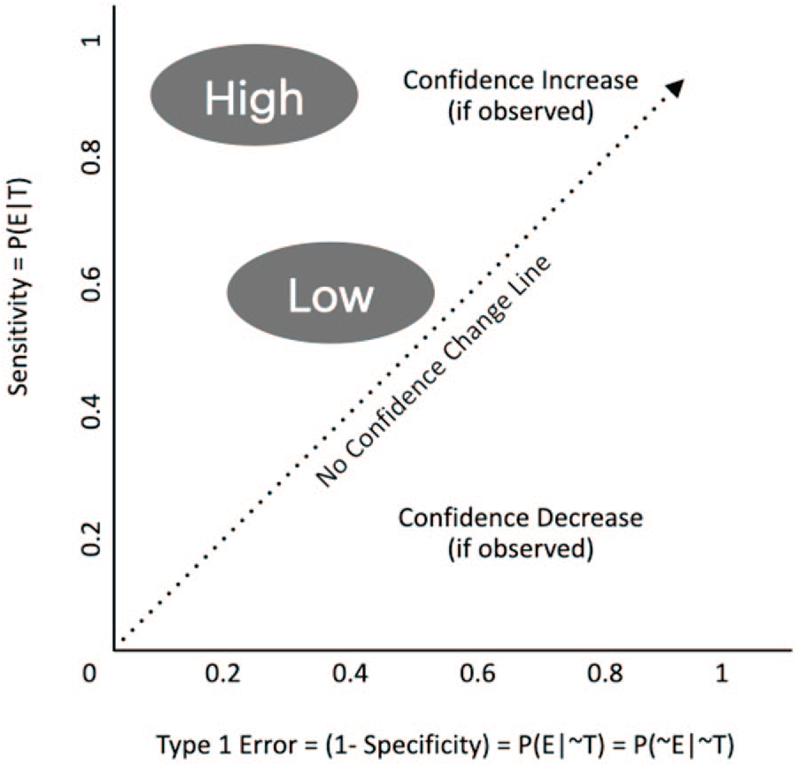
The model used here is an epidemiological model of a flu pandemic, investigating preventive behaviours and their influence on the course of the pandemic. It is a simplified version of the TELL ME model of communication about influenza (Badham and Gilbert, 2015), which was designed with epidemiology and communication experts from academic and policy making realms. This version (Badham, 2019, model version 3) has the communication elements removed but otherwise uses the same decision rules and empirically derived parameters as the full TELL ME model. The model comprises two interacting layers (Figure 2). One layer consists of simulated individuals that perceive their situation and make decisions about whether to adopt protective behaviour. For this example, the protective behaviour is assumed to be vaccination, but the behaviour is generic and could be reducing contacts or improving hand hygiene.
Influences within the agent-based model of protective behaviour decisions (from Badham, 2019, Figure 1.9, (creative commons licence)).
This behaviour is founded on a hybrid psychological model that includes attitudes, subjective norms and perceived threat as the key mechanisms in vaccination decisions. Each time step, each simulated person calculates a weighted average of their own attitude to vaccination (a value between 0 and 1), the proportion of nearby people who have adopted the behaviour (a proxy for norms) and a threat score. The threat score is the discounted cumulative local incidence of influenza; it increases as new cases occur and the contribution of previous cases decreases over time. Therefore, the threat score is high near the epidemic frontier and lower elsewhere. If the weighted average of these components exceeds some threshold (set at 0.4 for this study), the person seeks vaccination, which is assumed to be available.
The other layer is a spatial epidemic simulation. Standard epidemiological mathematical equations (Keeling and Rohani 2008) are used to estimate the number of newly infected people in a region in the next time step, based on the existing number of infected and susceptible people and a travel parameter that allows the epidemic to spread.
The epidemic layer influences the behaviour layer through the threat score, which keeps track of the number of infections. In the other direction, the adoption of protective behaviour by the individuals in a region affects the spread of the epidemic in that region. See Figure 2 for an outline of the mechanisms in the model.
We selected this model for its simplicity and therefore suitability to demonstrate how computer-based simulation can be used to support Bayesian updating by providing in silico frequencies to inform the prior probabilities. It is not intended to be a realistic representation of people’s behaviour in an epidemic. Despite its simplicity, however, the model displays all the features of a complex system that make causal attribution difficult in evaluation. Individual decisions are influenced by personal characteristics (attitude) and social pressures (the proportion of people nearby already vaccinated). The combined vaccination decisions of individuals affect the macro phenomenon of the epidemic spread and those decisions also respond to this macro phenomenon (through the threat score).
Estimating Bayes probabilities using the TELL ME model
Let us imagine that an epidemic has occurred for which a vaccine was available. We can collect data to estimate the number of people who were ever infected. Using that information (and assuming our behaviour model is correct), we can estimate the efficacy of vaccination using the frequencies generated in simulation experiments. We are comparing three hypotheses about how well the vaccine protects, efficacy values of 0.8, 0.9, and 1.0. These values can be interpreted as standard, improved and ideal vaccine efficacy levels. To demonstrate how the combination of the simplified TELL ME model and Bayesian Updating can help adjudicate among different claims, we showcase how the formula values would be calculated and confidence updated for observed values of the final proportion of infected population. Note that the ABM is seen as an additional tool to this estimation rather than a replacement to expert estimation. It can be seen as an in silico generation of proxy frequencies that are not otherwise obtainable in single case analyses.
Setting the model to represent these three hypotheses, we have three different but overlapping probability distributions of the final proportion of population ever infected (see Figure 3), with expected values of respectively, 0.33, 0.30, and 0.27. If the final proportion of ever infected population is higher than 0.33, we know with certainty that efficacy is 0.8 or lower. If it is lower than 0.26, we know with certainty that efficacy is 1.0. However, if the observed value of the infected population is between 0.26 and 0.33, there is some uncertainty as to the efficacy value. If it is in the range 0.26 to 0.275, efficacy could be either 0.9 or 1.0 (the overlap or intersection of the two distributions and excluding the distribution for efficacy of 0.8); if it is in the range 0.31 to 0.33, efficacy could be either 0.8 or 0.9. Finally, for values between 0.275 and 0.31, each of the three hypotheses is a possibility.
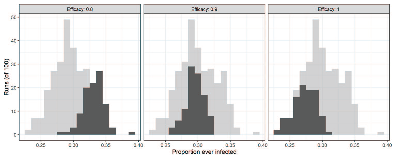
The proportion of the population ever infected under three parameter combinations. We have non-reversible protective behaviour (i.e. a vaccine) with vaccine efficacy of 0.8, 0.9 or 1. The outcome distribution of all experiments is displayed (light grey), highlighting the distribution associated with a specific efficacy parameter (dark grey).
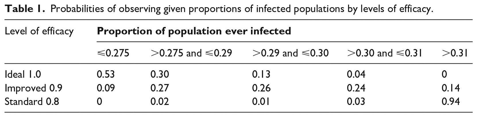
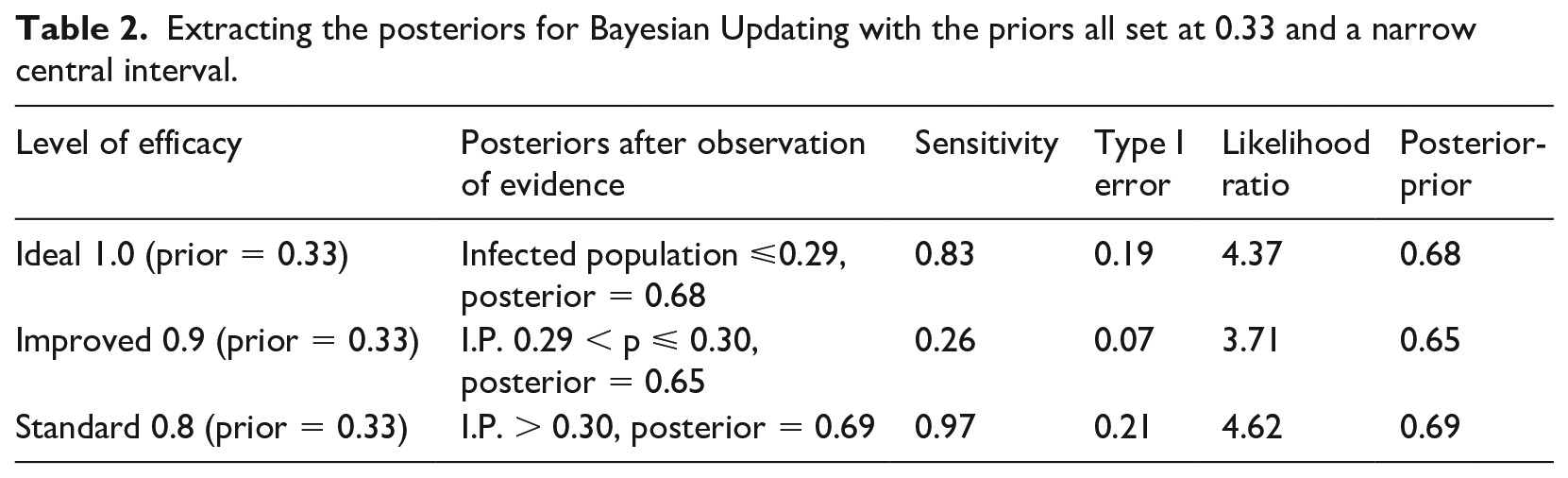
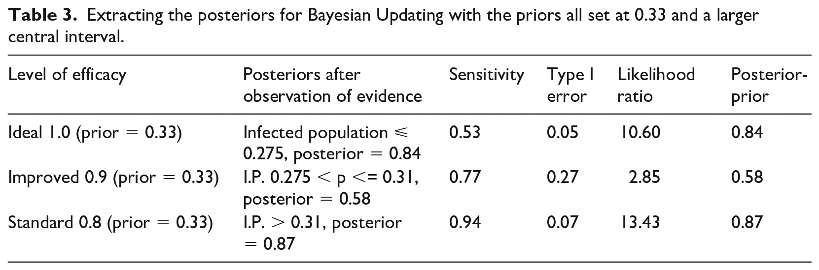
We split the most uncertain interval of 0.275 to 0.31 into three sections ( 0.275-0.29; 0.29-0.30; and 0.30-0.31) and calculate the probability of observing values within those ranges and outside under the three hypotheses (Table 1). We then consider two sets of ranges to test the level of efficacy: in the first case we take ⩽0.29 as an indicator of ideal efficacy; between 0.29 and 0.30 as an indicator of improved efficacy, and >0.30 as the best test for standard efficacy (Table 2). The central interval is relatively narrow here so we also consider alternative tests with a larger central interval of 0.275-0.31, the results of which are reported in Table 3.
Probabilities of observing given proportions of infected populations by levels of efficacy.
Extracting the posteriors for Bayesian Updating with the priors all set at 0.33 and a narrow central interval.
Extracting the posteriors for Bayesian Updating with the priors all set at 0.33 and a larger central interval.
Sensitivity is calculated by estimating the probability of observing an empirical proportion of infected population lower than a certain value under the assumption of ideal efficacy (efficacy = 1); higher than a certain value under the assumption of standard efficacy; and comprised within a range under the assumption of improved efficacy. Type I error is calculated by estimating the probability of observing an empirical proportion of infected population lower than a certain value under the assumption of improved or standard efficacy (the opposite of ideal), higher than a certain value under the assumption of either ideal or improved efficacy (the opposite of standard), and comprised within a range under the assumption of either ideal or standard efficacy (the opposite of improved).
The posterior values represent our updated (from a prior of 0.33) confidence that (1) efficacy is ideal if we observe a proportion of infected population lower than a certain value; that efficacy is standard if we observe a proportion of infected population higher than a certain value; and that efficacy is improved if we observe a proportion of infected population falling within a specific range.
Notice how the second set of tests is stronger at the extremes in terms of probative value than the first set of tests (final column, Table 3 compared to Table 2), because our confidence is raised to 0.84 and 0.87 instead of 0.68 and 0.69. However, for the improved value of efficacy, the first set of tests is slightly preferable, raising confidence to 0.65 instead of 0.58. This is understandable since the second set of tests has narrower intervals at the extremes, and the first set has a narrower central range: the narrower the test range, the higher its specificity and hence its confirmatory power.
The probative value of the two sets of tests is also expressed through the likelihood ratio: these confirm the superiority of the second set at the extremes (10.60 and 13.43 instead of 4.37 and 4.62) and of the first set for the central hypothesis and values (3.71 vs 2.85).
Conclusion
This paper aimed at contributing to the debate around what constitutes credible evidence in TBE, which has practical implications for decision-makers and for the use of evaluations. Building on the idea that TBE should be ‘diagnostic’ and should draw on Bayesian logic, we presented a way of supporting the Bayesian logic of Diagnostic Theory-Based evaluation with simulation data. There are two main ways of estimating the probabilities required by the Bayes formula: empirical frequencies and/or expert opinion. Computer-based simulation is a ‘third way’, which can be used to generate artificial data informing the association between particular outcomes and theories. Simulation provides a sophisticated way of combining objective and subjective understanding of the causal narrative. By simulating assumptions of mechanisms and relationships in silico, the method provides estimates for the sensitivity and Type 1 error of a piece of evidence for a particular hypothesis.
This demonstration used a simplified ABM of vaccination in an influenza pandemic (Badham and Gilbert, 2015), reasoning backward from the number of people infected in the course of the epidemic to the efficacy of vaccination. The population outcomes were divided into low, medium and high infected proportions to calculate the sensitivity and Type I error for three levels of efficacy. Calculations were executed with two different sets of intervals, one with a narrow middle interval, one with a wider one. The first set was discovered to be preferable – or ‘stronger’ in terms of probative value – for improved efficacy, while the second set was stronger for standard and ideal efficacy. In summary, if an evaluator was confronted with a given value of infected population, this method could be used to infer the vaccination efficacy with a given level of confidence.
The example model is intentionally simple as its main purpose is pedagogical: our aim was to provide proof-of-concept that simulated data can be used to estimate probabilities that change our confidence that certain theories or hypotheses are true (or false). When transported to the world of real-life evaluations, complications might arise as theories might be more complex or complicated. Such complications, however, would not result from applying Bayesian logic to the model, but from taking account of complex realities just like any other TBE would do. We therefore do not believe that, in itself, the approach would compromise the feasibility of evaluations. In other words, if we were trying to formulate a Theory of Change with an ABM, the difficulties we would encounter are related to the model’s creation, usability, and representativeness; not to the fact that we would use it to estimate Bayesian probabilities. If the model is low quality, then this endeavour would also suffer as the utility of the simulation output would depend on the quality of the theoretical representation; but this is true for all methods and in particular, for all ways of formulating theories of change, be it in Context Mechanism Outcome form, as a causal process mechanism, or as a contribution story mapping sequences of intermediate outcomes.
The purpose of this paper was to expand options for supporting probability estimation in Bayesian Updating. We used a proof-of-concept demonstration of how an ABM can be used to generate frequency distributions in silico. While we used an ABM, any model that can produce artificial data with probabilistic outcomes (like microsimulation or discrete event simulation) would also be suitable. When working with explicit numerical estimates, computer-based simulation with its ability to represent theoretical assumptions and explanations of how systems operate, offers a much-needed expansion opportunity to the Bayesian evaluator’s toolkit.
Footnotes
Declaration of conflicting interests
The author(s) declared no potential conflicts of interest with respect to the research, authorship, and/or publication of this article.
Funding
The author(s) disclosed receipt of the following financial support for the research, authorship, and/or publication of this article: This research was part funded by the ESRC Project Centre for Evaluation of Complexity Across the Nexus ES/S007024/1