
Abstract
This article discusses several practical issues arising with the application of diagnostic principles to theory-based evaluation (e.g. with Process Tracing and Bayesian Updating). It is structured around three iterative application steps, focusing mostly on the third. While covering different ways evaluators fall victims to confirmation bias and conservatism, the article includes suggestions on which theories can be tested, what kind of empirical material can act as evidence and how to estimate the Bayes formula values/update confidence, including when working with ranges and qualitative confidence descriptors. The article tackles evidence packages (one of the most problematical practical issues), proposing ways to (a) set boundaries of single observations that can be considered independent and handled numerically; (b) handle evidence packages when numerical probability estimates are not available. Some concepts are exemplified using a policy influence process where an institution’s strategy has been influenced by a knowledge product by another organisation.
Keywords
Introduction
Process Tracing with Bayesian Updating is increasingly popular as a methodological option in the evaluator’s toolkit. A companion article (Befani, 2020) has referred to it as a ‘diagnostic’ approach and linked it to the confusion matrix, discussing its benefits with regard to improving transparency, credibility and reliability of evaluation findings. However, the method presents a relatively steep learning curve and can run into a series of practical problems in some application settings. Once its logic and theory are understood, evaluators are often unsure how to estimate the probabilities required by the Bayes formula (in particular, Sensitivity and Type I Error); and some feel uncomfortable using numerical estimates at all. Another frequent roadblock are evidence packages: if evaluators are comfortable performing Bayesian Updating after new observations emerge, they might not be equally at ease handling multiple pieces of evidence assembled in a package.
This article provides suggestions on how to solve these problems, structuring the proposed solutions around three basic, iterative application steps: developing a testable theory; designing data collection; evaluating empirical data and updating confidence. All three steps come with perils in relation to confirmation bias (CB) and conservatism, which Bayesian Updating helps protect against (Befani, 2020).
Fighting CB and conservatism in practice
In the first application step, one or more propositions/statements are selected as theories to test. They can be developed as possible answers to evaluation questions, like ‘what role did the intervention play in achieving the outcome?’, ‘how did the intervention make a difference’ and so on. The idea of ‘testability’ is linked to standards of scientific quality like falsifiability and demonstrability 1 : a falsifiable theory can be rejected by potentially observable evidence. Not all theories are falsifiable: for example, ‘the programme had benefits’ is too ambiguous and vague to be falsified in this form, because even if the programme has been a disaster by most accounts, most likely it will have had some benefits for at least one person. A demonstrable theory can be demonstrated by potentially available evidence, but not all theories can: ‘the programme has been a tremendous success’ cannot be demonstrated unless the idea of success is unpacked and a specific definition is linked to observable data. In addition to sloppy theory definition, this step is subject to CB because of our tendency to select our preferred theories (in particular, to the search variant of CB). A high-quality application of Bayesian Updating should include formal testing of at least a handful of competing theories.
In Befani (2020) and throughout this article, we use as an example an influence theory stating that ‘our’ organisation (the one whose activity we are evaluating) has had an influence on another organisation’s policy or strategy. In order for this statement to be testable, more conceptual precision is required, for example, focusing on specific forms of influence that can be clearly identified and tested empirically, like the following: ‘this specific knowledge product has been used by this organisation in this way to produce this specific document, which has informed a process resulting in a specific section of their strategy’, and so on. This is preferable to vague, broad statements like ‘organisation X has influenced the policy of institution Y’. The advice here is to test whatever proposition we can convincingly demonstrate, even though their scope might be more limited than what we were initially hoping (see Box 1).
Box 1.
Summary of the main evaluation example used in the text.
S: Sensitivity; T1E: Type I Error.
In the second step, data collection is designed bearing in mind conclusive tests, that is, seeking to observe strong or high-probative-value evidence that can convincingly confirm or disconfirm the theory. CB is lurking here too: in our asymmetric hopes of strengthening versus weakening the theory, we might gravitate towards ‘love-to-see’ (Befani and Stedman-Bryce, 2017) Smoking Gun (SG)–like confirmatory evidence, rather than towards ‘hate-not-to-see’, disconfirmatory Hoop tests (HTs). In order to shun accusations of CB (Wauters and Beach, 2018) we should seek ‘hate-not-to-see’ HTs, as much as we seek ‘love-to-see’ or ‘wish-to-see’ SGs. We should ensure that the search for observable HTs has been thorough, as opposed to the theory not being weakened for lack of trying.
Continuing with both our medical and evaluation examples, a doctor making a diagnosis should use both specific and sensitive tests and hope to observe both positive specific tests (that would confirm the diagnosis) and negative sensitive tests (that would rule out the diagnosis). In our policy influence evaluation, we should both seek matching text in the relevant documents (and hope to find a large amount of it, that would confirm the influence theory) and hope to find strong differences in content (that would rule out the hypothesis of influence).
Finally, formal Bayesian Updating is conducted by applying the Bayes formula, estimating Sensitivity and Type I Error, and obtaining the posterior, post-observation level of confidence (Befani, 2017; Befani and Stedman-Bryce, 2017). This can be undertaken for different theories and statements, 2 adjudicating among them on the basis of our post-observation confidence. In Table 1, for example, we would choose or prioritise Theory Two.
Confidence levels in statements/theories before and after data collection.
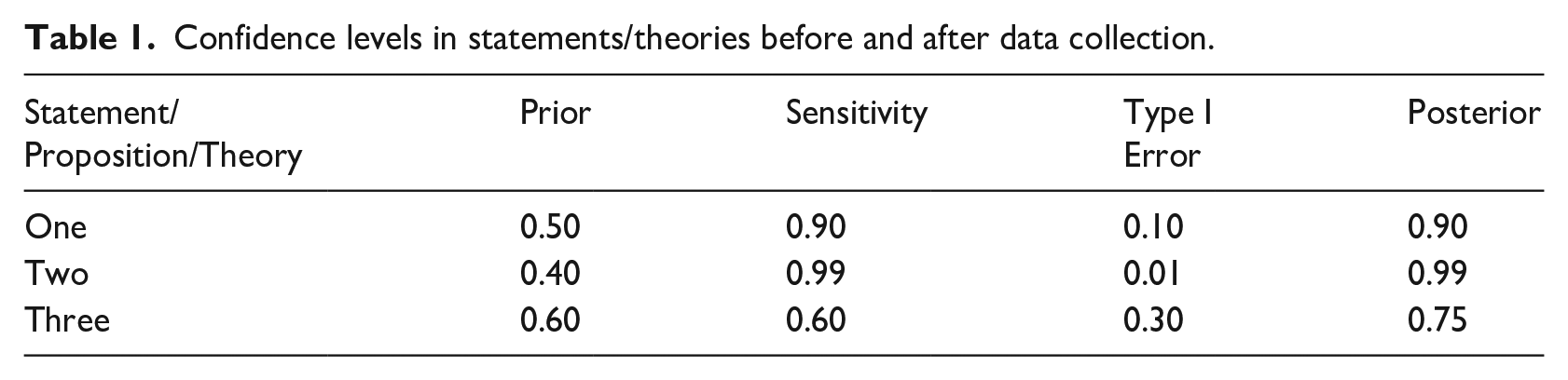
Here, a variety of CB forms conjure to underestimate Type I Error (see Box 1): for example, we can fail to recall events linked to alternative explanations or theories that can produce the assessed observations as much as the theory under investigation. Failing to remember the existence of an alternative knowledge product, perhaps published by another organisation, with a similar content that the institution could have been influenced by, could be an example of Memory Confirmation Bias. An example of Search Confirmation Bias is when, if the institution has had contacts with several think tanks in the lead up to the strategy formulation, the evaluator would normally not devote the same energy to investigating and analysing the linkages between the institution and all of these organisations, giving priority to studying their preferred organisation. Analysis Confirmation Bias could manifest itself when the evaluator is exposed, for example, to a (theoretically influenced) stakeholder that they know has good relations with the (theoretically influencing) organisation, and the stakeholder is claiming that their institution was influenced by the former. An evaluator victim of CB might tend to consider that a SG, downplaying or even failing to consider any external motivation the stakeholder might have had; while another, more cautious, evaluator would consider alternative motivations more seriously and downplay the confirmatory power of that observation.
CB (in all its forms) tends to underestimate the Sensitivity values because higher values would make it easier for the theory to be rejected if HTs are not observed: which is something that we might unconsciously fear. Search bias makes us reluctant to seek HTs and Analysis bias makes us underestimate Sensitivity values so that, even if we fail to observe HTs, we can still hope that the theory is true. These considerations suggest that, for our preferred theories or for theories that commissioners have a stake in confirming, high values of both Sensitivity and Type I Error should be trusted more than low values; and the latter should raise suspicions of CB.
Estimating the probabilities required by the Bayes formula
Formal updating requires using the Bayes formula, that is, estimates of Sensitivity and Type I Error. The latter are probabilities of observing the evidence under the assumption that, respectively, the theory is true, and that it is not. Two of the most common ways of thinking about probabilities are as an observed, empirical frequency (the number of times an event occurs, out of the number of times it could potentially occur) and as subjective probability (someone’s more or less informed opinion on the event’s likelihood of occurring). A third way is ‘simulated frequency’, or probability as the observed frequency of an indicator when running a simulation model multiple times (Befani et al., forthcoming).
The first kind (a.k.a. frequentist probability) is arguably the easiest to understand and use, but in many evaluations, the relevant empirical data are not available. In medical diagnosis, Sensitivity and Type I Error can be empirical frequencies because the number of patients exhibiting positive and negative values of specific tests can be counted; and it can also eventually be known who, among them, had or did not have a specific disease. The third kind is in the early stages of being developed (Befani et al., forthcoming) so we will focus mainly on subjective probability.
The literature on eliciting probabilities from experts is vast and long-standing (Cooke, 1991; EFSA, 2014; Gosling, 2014; O’Hagan and et al, 2006; Oakley and O’Hagan, 2016). It discusses elicitation of probability distributions and different ways to express probability judgements and their implications, as well as how to extract, calibrate and assemble expert judgements.
O’Hagan et al. (2006) provide a useful list of the several different ways statements about chance and uncertainty can be expressed: as probabilities, percentages, relative frequencies, odds or natural frequencies. Box 2 illustrates how we would express uncertainty around observing matching text as a piece of evidence.
Box 2.
Different ways of expressing probability judgements.
Probability: ‘there is a 0.05 probability of observing (this amount of) matching text under such conditions if the influence theory is not true’.
Percentage: ‘there is a 5% chance of observing (this amount of) matching text under such conditions if the influence theory is not true’.
Relative frequency: ‘under such conditions, we would observe (this amount of) matching text one in 20 times the influence theory is not true’; or ‘we would observe (this amount of) matching text 50 times every 1000 times that the influence theory is not true’.
Odds: ‘if the influence theory is not true, the odds against observing (this amount of) matching text are 19 to 1’.
Natural frequency: ‘from a sample of 100 similar policy processes where two organisations did not influence each other, (the same amount of) matching text between their products was observed 5 times’.
There is cautious consensus that using frequencies (in the way subjective probability is expressed) improves accuracy (base rate, no misunderstandings about the reference class), although there are some important exceptions to this (O’Hagan et al., 2006).
Some well-known elicitation procedures are the Sheffield method (a.k.a. SHELF) (Oakley and O’Hagan, 2016); Cooke’s method (Cooke, 1991); and the Delphi method (EFSA, 2014). They mainly differ on whether and how experts are allowed to interact and exchange views: no interaction for Cooke’s method (mathematical aggregation); full interaction for Sheffield (behavioural aggregation); and a more limited, controlled interaction for Delphi, a middle ground between the first two methods. The methods take account of, and fight in different ways, typical biases involved in eliciting probabilities: for example, overconfidence, anchoring and adjustment, availability, and representativeness.
Experts can be asked to express multiple single probabilities (that would be assembled into distributions in the post-elicitation phase) or plausible ranges. It is the author’s opinion that ranges, in particular, when associated with qualitative descriptors of confidence levels (see next paragraph), can work for a wide range of evaluation processes, including those that cannot afford pre-training in quantitative elicitation and probability theory. The existing, well-established elicitation methods can thus be adapted for evaluation purposes, while preserving their bias reduction strategies.
Working with ranges and qualitative levels of confidence
If evaluators are uncomfortable working with point estimates, Bayesian Updating can also be carried out using ranges of values. 3 Probability estimates, however, do not have to be numerical: they can also be expressed qualitatively, for example ‘highly confident that the event will happen’ or ‘more confident than not that the event won’t happen’. These qualitative confidence descriptors can be associated with numerical intervals/converted into quantitative ranges (see Figure 1 and Table 2 in Befani, 2020), 4 and Bayesian Updating can be carried out using the extreme ends of the range. The rest of the paragraph will show how to do this, step by step.
Unless the evidence is uninformative, we would normally have two different ranges or qualitative estimates for Sensitivity and Type I Error: for Sensitivity, let us assume that we are ‘highly confident’ that we will observe the evidence if the theory is true (0.85–0.95); and that, for Type I Error, we are ‘reasonably certain’ that we will not observe the evidence if the theory is false (0.01–0.05). These two ranges have four extremes and create four reference scenarios, with infinite possibilities in between (Table 2).
Four scenarios created by estimating confidence qualitatively.
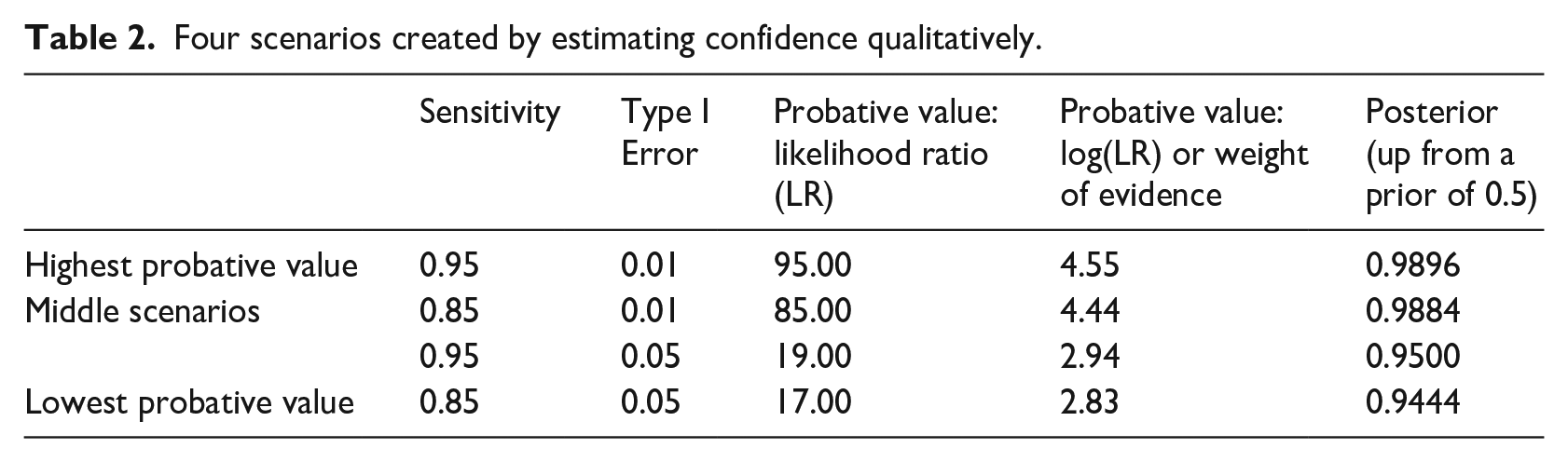
The probative value continuum ranges from the high peak, where Sensitivity is highest and Type I Error lowest (the strongest evidence scenario with a weight of evidence 5 of 4.55 and a likelihood ratio of 95.00), and the low peak, where Sensitivity is lowest and Type I Error highest (the weakest evidence scenario with a weight of evidence of 2.83 and a likelihood ratio of 17.00). The posterior confidence is also returned as an interval, ranging from a minimum of 0.9444 in the most unfortunate case, to a maximum of 0.9896 in the best scenario.
The above example shows that if we do not identify point estimates but are comfortable with probability ranges, we can learn from Bayesian Updating that, for example, our post-observation confidence does not fall below a certain lower limit, nor rise beyond a given upper threshold. And if we are still uncomfortable with numbers, we can translate the posterior range back into a qualitative descriptor: in our example, 0.94–0.99 almost entirely overlaps with ‘reasonable certainty that the theory is true’ (second row of Table 2 in (Befani, 2020), see also first row of Table 3 below). If the numerical range covers two qualitative descriptors, we can choose the one that the range overlaps with more extensively: for example, if we had 0.87–0.97, we could pick ‘high confidence that the theory is true’. Or, if we want to be more conservative and are interested in worst-case scenarios, we can pick the lowest qualitative descriptor overlapped by the range (see Table 2 in (Befani, 2020) and Table 3 below).
Bayesian Updating with qualitative statements. a
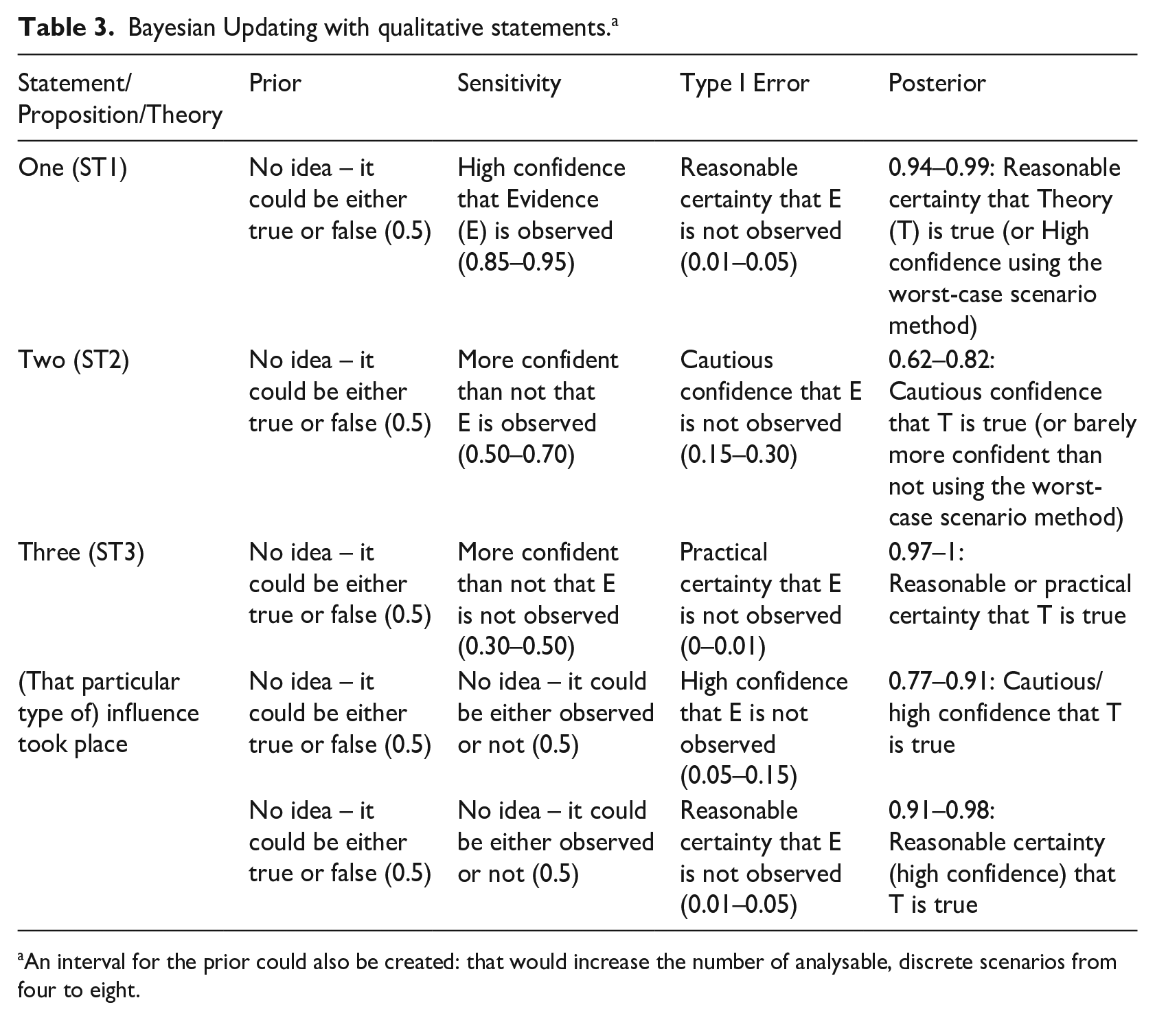
An interval for the prior could also be created: that would increase the number of analysable, discrete scenarios from four to eight.
In our policy influence example, we can estimate the Sensitivity and Type I Error of ‘relatively large amounts of text matching’ for our hypothesis of influence being true in the following way. For Sensitivity, we can argue that ‘if [that particular kind of] influence took place, we are neither confident nor not confident that such amount of text matching would be observed’ (corresponding to 0.5, so no range in this case but a point estimate). For Type I Error, we can argue that ‘if that institution’s strategy was not influenced by our organisation’s knowledge product, we are highly confident (or perhaps reasonably certain) that such amounts of identical text would not be observed’. This would set Type I Error between 0.05 and 0.15 (or between 0.01 and 0.05 if we are reasonably certain). Our posterior confidence that the theory is true would then be between 0.77 and 0.91 (or between 0.91 and 0.98 with the reasonable certainty estimate). If we translate the first interval into a qualitative descriptor using the first method described above, we can conclude that we are between cautiously confident and highly confident that influence took place because the range 0.77–0.91 overlaps these two descriptors (0.70–0.85 and 0.85–0.95) to the same extent. If we use the worst-case scenario method, we conclude that we have only reached ‘cautious confidence’ because 0.77 is included in this bracket. For the second estimate giving us a posterior of 0.91–0.98, if we use the first method, we can conclude that we are ‘reasonably certain’ because the interval overlaps to a larger extent with 0.95–0.99 than 0.85–0.95 (high confidence); or that we are only ‘highly confident’ if we use the second method (0.91 falls within 0.85–0.95).
A freely available tool for Bayesian Updating (Befani, 2017) currently offers the opportunity of working with qualitative levels of confidence for Sensitivity and Specificity: it converts them into numerical ranges and then computes the corresponding range for the updated confidence or posterior. 6 The numerical range can then be converted back into the qualitative descriptor, as we see in Table 3.
When expressed as above, our estimates and judgements are transparent and falsifiable: for example, they can be challenged by arguing that observing the same amount of text matching, if influence has not taken place, is not as rare as assumed. The challenging stakeholder can provide evidence to support their estimate. In probability elicitation techniques where stakeholders/experts are allowed to interact, this kind of discussions will take place before a consensus is reached.
Working with evidence packages
In any given evaluation, it is very unlikely we will observe only one piece of evidence: normally, our data collection and desk reviews produce several individual interviews, include documents, perhaps focus groups. Similarly, in a medical diagnosis, the physician might consider a combination of symptoms, blood tests results and diagnostic images like X-rays, MR scans and so on.
At the same time, it is good practice to be assessing different, sometimes even mutually exclusive, theories. For example, when investigating our influence theory, we should be open to the idea that the institution’s strategy has not been influenced by that knowledge product but by other products or processes apart from the institution; and we should be equally thorough in investigating these options.
In principle, different pieces of evidence have different diagnostic value for the same theory, and the same piece of evidence has a different diagnostic value for different theories: a knowledge product by organisation A is likely not to be informative about the influence of organisation B. Similarly, different stakeholders with knowledge of different processes and organisations provide information which most likely will not be (equally) useful for all theories or hypotheses. In medical diagnosis, diagnostic images are more reliable than blood tests results for certain conditions. In sum, the same observation can be strong evidence for a theory and weak evidence for another theory 7 ; and different pieces of evidence increase or decrease confidence in the same theory to different degrees.
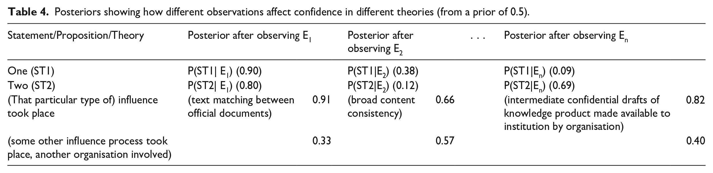
Before discussing evidence packages, it is important to untangle this complexity by showing that each level of posterior confidence is associated not just to one single piece of evidence but also to one single theory or statement: Table 4 provides data from two hypothetical examples plus two influence theories. If we look at the first theory, it is supported by E1 and weakened most strongly by En; while the second theory is supported by E1 and weakened most strongly by E2. E1 strongly supports our influence theory, while E2 is inconclusive for it. As for pieces of evidence, E1 supports Theories One and Two and the first influence theory, but not the second one; En very mildly supports Two and strongly weakens One, and so on.
Posteriors showing how different observations affect confidence in different theories (from a prior of 0.5).
Considering each piece of evidence in relation to one theory at a time requires calculating one value of Sensitivity and one value of Type I Error for each observation, one theory at a time. In principle, each observation has a different Sensitivity value for the same theory: if our influence theory is true, we expect to see a broad consistency in the content of the two documents (with 0.95 probability, see Box 1 and Supplemental Table S1) but not necessarily a perfect matching between (large) portions of text (0.5). A single observation also has different Sensitivity values for different theories: the previously considered matching text between the two documents has a different probability of being observed under the assumption that the posited influence theory is true (0.5 in Supplemental Table S1), than under the assumption that a different theory is (0.1): if the institution was influenced by another organisation, the probability of observing (large amounts of) text matching the other organisation’s knowledge product is much lower.
The same distinctions need to be made for Type I Error values (Supplemental Table S2): each observation has different Type I Error values for the same theory. If our influence theory does not hold, observing (large portions of) matching text is quite unlikely (0.05); but the probability that the two organisations exchanged drafts at some stage, without the institution being influenced by the content of the knowledge product, is higher (0.15). And broad alignment in content should not be a surprise, particularly if the same position is widely shared among a group of institutions (0.5, see Box 1). In addition, the same observation (let’s say, matching text) has different Type I Error values for different theories: if our influence theory is not true, matching text is quite unlikely (0.05); but if the alternative influence theory is not true, which includes the possibility of our influence theory being true, matching text becomes more likely (0.2).
The cells of Table 4 are obtained by updating the priors for the statements/propositions/theories on each row with the Sensitivity values of Supplemental Table S1 and the Type I Error values of Supplemental Table S2. If we look at Table 4 by column, we can see that the theory most strongly supported by matching text is our influence theory (0.91), with Theory One a close second (0.90). The least strongly supported is the second influence theory (0.33). The two other pieces of evidence also support our influence theory more strongly than the other three theories. If we look at rows, we can see that the strongest evidence for our influence theory is matching text (0.91 posterior confidence); followed by exchange of confidential drafts (0.82). The weakest piece of evidence is broad content consistency (0.66), which is a good HT but is not very informative when observed.
We are now ready to discuss evidence packages, or the simultaneous assessment of multiple observations. The above considerations might sound abstract because they refer to the assessment of single observations, as if we collected only one piece of evidence at a time; as if, every time we made a new observation, we forgot the previous one. For example, the ‘posterior after observing E1’ (the matching text) is based on E1 and E1 only, as if E2 (broad content consistency), . . ., En (exchange of intermediate drafts) and so on did not exist. In reality, we almost always collect multiple pieces of evidence, so we need a procedure to group our estimates together.
The rest of the article will address multiple ways to approach the assessment of evidence packages. If we have enough resources to carry out formal Bayesian Updating, we have four options:
If we manage to define some observations as independent from each other, we can multiply their (previously discussed) single-piece estimates;
If we cannot draw independence boundaries among some observations, we can Consider a group of (inter-dependent) interviews, documents and so on as one single piece of evidence; Multiply the single-piece estimates as in (1) but using discount factors to reduce the probative value proportionally to the degree of inter-dependence Calculate the conditional probabilities of observing each single piece of evidence after having observed others (under the two hypotheses of the theory being true and not being true).
If probability estimates are not available or cannot be obtained, we can create rubrics defining different degrees of empirical support for the theory (option 5). Option 2a is not technically different from what we have seen so far, and option 2b is currently being developed; therefore we illustrate options 1, 2c and 5.
Working with evidence packages when Bayesian estimates are available
If numerical estimates are available, we can formalise the evidence package as ‘E1∩E2∩ . . . ∩En’; or the combination of empirical observations E1, E2, . . . En (Supplemental Table S3). We can then estimate the Sensitivity and Type I Error of the package in relation to different theories. This will be done differently depending on whether the pieces of evidence can be argued to be stochastically independent or not. 8
The general formula for calculating the probability of combined, multiple events requires calculating the probability of making a given future observation on condition of having already made specific ones (Dekking et al., 2006). For example, if we have already observed E1, the probability of also observing E2 is P(E2|E1). The probability of subsequently observing E3 is P(E3|E2∩E1), and so on, until P(En|En-1∩En-2∩ . . . ∩E1) which is the probability of observing En after having made the previous n-1 observations. For our purposes, we would need to calculate the conditional Sensitivity values (see Supplemental Table S4) and the conditional Type I Error values (Supplemental Table S5). It is possible but potentially quite cumbersome to calculate these conditional probabilities for each piece of evidence and each theory; as we mention above in option 2a, a relatively acceptable shortcut is to consider the whole package as one single piece of evidence and calculate two single values to feed into the Bayes formula (D’Errico et al., 2017).
If observations are independent, 9 however, we are offered a mathematically formalised shortcut since the conditional probabilities will be equal to the non-conditional ones, which are likely to be already available at this stage. We can thus calculate the probability of observing a combination of observations (or the probabilities of a package) by multiplying the probabilities of observing the single pieces (Supplemental Tables S1 and S2). In particular, the Sensitivity of a package will be obtained as the multiplication of Sensitivity values of the single pieces (see Supplemental Tables S4 and S6), and the Type I Error of the package will be obtained by multiplying the Type I Error values of the single pieces (Supplemental Table S5 and S7).
In medical diagnosis, scan machines and lab processes ignore each other, so it is easy to argue that findings from blood tests are independent from findings from imaging tests; another example of independent events being when we interview informants whose opinions have not been influenced by each other. In our evaluation example, however, while relatively large amounts of matching text between documents are quite rare an occurrence, our expectation of those might be slightly increased if we observe broad content alignment first, because we assume the document authors to be responsible for both. And if we see that there was a document exchange at the beginning involving the authors, we expect broad content alignment more than if we did not see the former. However, for illustration, let us assume that we can argue for stochastic independence among these three observations so we can apply the procedure and calculate the Sensitivity of the three piece-package by multiplying the Sensitivity values of the single observations constituting the package (as in Supplemental Table S6).
If conditioning on the theory being false (as opposed to being true as above) does not change our independence assumptions on the evidence pieces, we can calculate the Type I Error of the package in the same way, by multiplying the Type I Error values of the single package components (see Supplemental Table S7). The posteriors in the last columns of Supplemental Table S3 are then obtained from the Sensitivity values of Supplemental Table S6 and from the Type I Error values of Supplemental Table S7.
In general, if observations are independent under the theory, it does not necessarily imply that they are independent under alternatives to the theory: so we might be able to use this method to calculate the Sensitivity of the package, but not the Type I Error, or vice versa. For example, if employees of an organisation are interested in showing that the theory is true but unfortunately it is not, they might have more incentives on presenting an agreed, positive view during interviews, compared with a situation where the theory is actually true and they are more relaxed about agreeing on what to say during evaluation-related interviews. The simple multiplication method only works if pieces of evidence are independent, conditioned on the theory-related hypothesis. However, a procedure currently being developed by the author assigns discount coefficients to single-piece values when observations present some degree of inter-dependence (between full independence and full inter-dependence) and would allow evaluators to use the transparent “mathematical multiplication” option in the relatively common situation where the observations cannot be considered either fully independent or fully inter-dependent under at least one of the two hypotheses (theory true and not true).
The wonders of discovery (or of reducing uncertainty)
Not rarely, Bayesian Updating yields surprising or unexpected findings because of our poor ability as humans to sufficiently update our beliefs on the basis of emerging empirical evidence. But Bayesian Updating performed on combined, multiple independent observations potentially produces even more counterintuitive findings because our inaccuracy and bias only get larger and more serious as the number of observations increases.
The two typical cases where uncertainty (and hence, potentially, surprise) are maximised are when (a) we handle mixed or seemingly contradictory evidence, with some pieces strengthening and others weakening the theory, and (b) when we are presented with multiple weak pieces of evidence that all seem to lean in the same direction (either all for weak confirmation or all for weak disconfirmation).
In the first case, we might know that one piece weakens and another strengthens the same theory, but we usually cannot tell if the former weakens more strongly than the latter strengthens. This gets a lot more complicated with more than two observations. Let us take the case of Theory/Statement/Proposition One in Table 4: E1 increases our confidence (0.90), but E2 (0.38), and most of all En (0.09), decrease it. Without Bayesian Updating, our verdict would simply be ‘mixed evidence’ or ‘contradictory evidence’; but most of the times the evidence is more informative than we think, and the actual posterior after observing the package is 0.36, which is lower than we were probably expecting. If we use the currently available tools to automatically check the direction and strength of the evidence package, we often discover that it is more conclusive, and perhaps in a different direction, than we expected. In other words, humans’ idea of uncertainty or mixed evidence tends to be anchored more closely to the 0.5 middle point than it should be.
As for the second situation where observations are all of the same kind (say, all strengthening), but are individually weak, it is difficult to accurately know how strong the package is unless we use the formula (and, for independent observations, the automatic combination function of the tool). Due to conservatism, humans tend to underestimate the power of evidence to change their priors, and they will usually be surprised at how strongly conclusive a package comprised of three or four weak straws of the same kind can be. And even those humans less subject to this bias will not know how many straws of the same kind they need (say, similar responses in independent interviews) to reach a certain level of overall confidence, unless they use the formula.
In our influence theory case, the three observations can be considered relatively weak; however, if we assume their independence and put them together, as a package, they are much stronger than any individual piece, almost achieving practical certainty (0.988). If we have multiple independent similar straws, say each having 0.6 Sensitivity and 0.4 Type I Error, while individually they would increase a 0.5 prior only to a 0.6 posterior, six of them are enough to achieve a 0.92 posterior, and 10 would raise it to over 0.98. Without Bayesian Updating, it would be very difficult to estimate how much our level of confidence should increase as more similar weak tests emerge during data collection.
How much evidence is enough?
Using Bayesian Updating to estimate the strength of evidence packages is also needed to test how sensitive our confidence is to possible new discoveries and can help answer the recurring question, ‘how much evidence is enough? When can we stop seeking and collecting?’ More specifically, this question 10 can become ‘how strong a piece of evidence from the opposite direction do I need in order to substantially change my assessment?’ The ‘cast the net widely’ suggestion (Bennett and Checkel, 2014a), encouraging us to consider the widest possible range of theories as well as pieces of evidence, rather than cherry-picking the ones that will confirm our favourite theory, now takes the form of a list, each item of which comes with an estimation of its strengthening (Type I Error) and weakening (Sensitivity) powers. Seeing only strengthening pieces in the package should create suspicions and make quality assurers enquire about what is possibly missing. Similarly, low estimates of Sensitivity and Type I Error should raise suspicions of Analysis and Memory Confirmation Biases, that make us overestimate the observations’ strengthening powers and underestimate its weakening abilities.
If the observations are not stochastically independent, for example, when informants are part of a working group that have collaborated during the project and are reporting a group position towards the programme, that perhaps they have also expressed in meeting minutes and other pieces of evidence, we either take the conditional probability approach (Supplemental Tables S4 and S5) or we consider the package as one single, complex observation; redefining the boundaries of pieces creatively and replacing the various estimates with a single one covering all the inter-dependent parts of the package (or – once it is fully developed – we could use the above mentioned, modified multiplication method). For example, if we have reason to believe that our three observations above are inter-dependent, we would calculate the Bayes formula values for a single comprehensive observation including matching text, broad content alignment and exchange of confidential drafts; or, in alternative, calculate the conditionals for observing text once we observe content alignment; of exchanging drafts once we observe the other two and so on. Despite being advocated elsewhere (Fairfield and Charman, 2017), so far, the author has found the latter approach mostly impractical in real-life evaluation settings: one major challenge being the consistency of the estimate for different ways that observations are ordered. Isolation of independent observations and wrapping of the residue into a single comprehensive estimate does not require ordering and is free from biases that change the estimate as the order of observations changes.
Working with evidence packages when Bayesian estimates are not available
When we are dealing with multiple, arguably independent pieces of evidence, but for various reasons, we are unable to produce estimates for Sensitivity and Type I Error, we can still combine the observations in a sensible way, provided we assign it Process Tracing (PT) test categories like SG, HT, Doubly Decisive (DD) and Straw-in-the-Wind (SW). 11
Building on pioneering work by (BEIS, 2018), we propose a way to establish the level of empirical support for a theory on the basis of multiple independent observations, of which we know the PT test category (see Table 5) but not the Bayes formula values. The system includes five levels of support for a particular theory T: strong support, possible support, contradictory support, possible support for the opposite theory and strong support for the opposite theory. We describe these levels in the rest of the section.
Assembling pieces of evidence in the absence of Bayesian estimates.
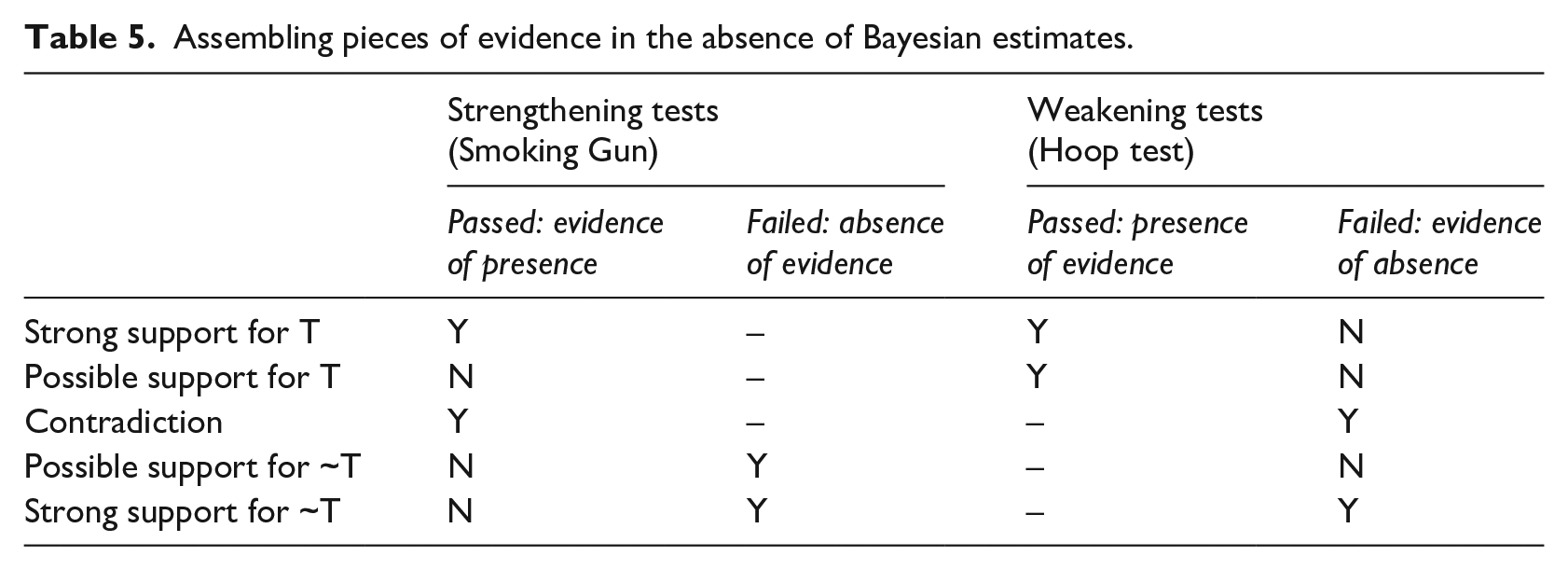
‘Strong support for the opposite theory’ (last row of Table 5) arises when the theory is weakened by the failure of at least one HT; at the same time, it is not strengthened because no SG is passed (with at least one having been tried and having failed). In other words, when we have evidence of absence (the HT fail) without having evidence of presence (no SG); plus some absence of evidence (the failed SG, see also Box 1). If we consider the matching text a SG and the broad content alignment a HT, this situation ( ‘strong support for absence of influence’) is equivalent to failing to observe broad content alignment, and also failing to observe matching text, with no other SGs passed.
At the other end of the spectrum, we witness ‘strong support for the theory’ (first row of Table 5) when at least one SG is passed, giving us ‘evidence of presence’; and no HTs fail, preventing us from finding evidence of absence. Since we are supposed to have tried some Hoops, at least one would have passed; hence, we also have presence of evidence. In our example, this is like when we observe matching text (a SG), and we also observe broad content alignment (a HT).
The above two cases are somewhat symmetrical; two of the in-between scenarios are also symmetrical, while the third is qualitatively different. In the ‘possible support for theory’ case (second row of Table 5), we observe some evidence (presence of evidence), but this is because some HTs are passed; not because any SGs are: the latter might not even be identified. The theory can be true: we have not been able to weaken it, but, unfortunately, we are not quite able to strengthen it either. This is like observing broad content alignment (HT) but failing to observe matching text (SG), or not even seeking to observe the latter.
The case of ‘possible support for the opposite of the theory’ (fourth row of Table 5) is similar: we can neither strengthen nor weaken the theory (we do not have evidence of presence or evidence of absence); but instead of passing HTs and having some weak evidence for the theory, HTs might not even be identified. SGs instead (at least one) are identified and fail, making us worry about absence of evidence. This is like seeking to observe matching text and failing, while not seeking to observe broad content alignment.
Finally, the contradictory case (third row of Table 5) is when at least one SG passes and at least one HT fails: producing the logical contradiction of witnessing evidence of presence and evidence of absence at the same time. This is like observing matching text but failing to observe broad content alignment. The theory and its opposite are seemingly equally supported.
The middle situations are the ones that benefit the most from formal Bayesian Updating, especially the contradictory case. In our example, if we consider only the first two observations, with Sensitivity values of 0.5 and 0.95, and Type I Error values of 0.05 and 0.5, observing 12 the first (SG) but not the second (HT) means that the two pieces neutralise each other and the posterior after observing them is identical to the prior (0.5). But with slightly different values that would not change our qualitative assessment of ‘contradictory case’, for example, sensitivities of 0.3 and 0.97, and Type I Errors of 0.1 and 0.4, making the first observation raises the prior to 0.75 and failing to make the second decreases it to 0.05, yielding a posterior based on the combined package of 0.13. Qualitatively, the two pieces of evidence would still be a SG and a HT, but while 0.5 in the first case conveys the uncertainty that we would normally associate with contradictions, the 0.13 of the second case is a pretty convincing disconfirmation of the theory.
Concluding remarks: Diagnostic evaluation is possible and necessary
Many of the benefits provided by diagnostic evaluation have been outlined in Befani (2020), including the minimisation of CB and conservatism. This article has shown how to apply the approach in practice, following the typical steps; addressing the many risks and types of biases arising along the way, and suggesting protective measures. We have shown how to formulate statements/propositions/theories, assign probabilities, work with qualitative confidence descriptors and how to handle multiple observations, a.k.a. evidence packages, including in the presence of weak or contradictory evidence.
Applying this approach potentially presents challenges, some of which seem to be more serious just when the approach is comparatively more useful, like in situations of weak or conflicting evidence that are at higher risk of bias. While diagnostic evaluation provides several practical opportunities to minimise both CB and conservatism, we find that the latter is particularly problematic, especially when we are confronted with seemingly inconclusive pieces of evidence; hence, we advocate increased precision in the characterisation of SW tests. The early literature on Process Tracing tests focused on extremes, which are relatively easy to identify, while reality is more often populated with middle grounds and in-betweens; and tests approximating straws abound.
The numerical formalisation of Bayesian Updating allows us to make more fine-grained distinctions among different inconclusive tests, allowing us to spot differences in terms of both strength and direction. This is essential when having to estimate the probative value and direction of evidence packages. In general, it is very difficult to predict how much adding one piece of evidence of a certain kind and strength, affects the kind and strength of an existing package. It can easily be seen by playing with the updating tool (Befani, 2017). Diagnostic evaluation reduces the uncertainty and confusion by letting the evidence speak for itself.
Supplemental Material
Supplementary_Tables_without_Highlights – Supplemental material for Diagnostic evaluation and Bayesian Updating: Practical solutions to common problems
Supplemental material, Supplementary_Tables_without_Highlights for Diagnostic evaluation and Bayesian Updating: Practical solutions to common problems by Barbara Befani in Evaluation
Footnotes
Funding
The author received no financial support for the research, authorship and/or publication of this article.
Supplemental material
Supplemental material for this article is available online.
Notes
References
Supplementary Material
Please find the following supplemental material available below.
For Open Access articles published under a Creative Commons License, all supplemental material carries the same license as the article it is associated with.
For non-Open Access articles published, all supplemental material carries a non-exclusive license, and permission requests for re-use of supplemental material or any part of supplemental material shall be sent directly to the copyright owner as specified in the copyright notice associated with the article.