On lower-dimensional models in lubrication,Part B: Derivation of a Reynolds type of equation for incompressible piezo-viscous fluids

Abstract

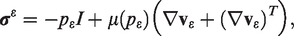
The Reynolds equation is a lower-dimensional model for the pressure in a fluid confined between two adjacent surfaces that move relative to each other. It was originally derived under the assumption that the fluid is incompressible and has constant viscosity. In the existing literature, the lower-dimensional Reynolds equation is often employed as a model for the thin films, which lubricates interfaces in various machine components. For example, in the modelling of elastohydrodynamic lubrication (EHL) in gears and bearings, the pressure dependence of the viscosity is often considered by just replacing the constant viscosity in the Reynolds equation with a given viscosity-pressure relation. The arguments to justify this are heuristic, and in many cases, it is taken for granted that you can do so. This motivated us to make an attempt to formulate and present a rigorous derivation of a lower-dimensional model for the pressure when the fluid has pressure-dependent viscosity. The results of our study are presented in two parts. In Part A, we showed that for incompressible and piezo-viscous fluids it is not possible to obtain a lower-dimensional model for the pressure by just assuming that the film thickness is thin, as it is for incompressible fluids with constant viscosity. Here, in Part B, we present a method for deriving lower-dimensional models of thin-film flow, where the fluid has a pressure-dependent viscosity. The main idea is to rescale the generalised Navier-Stokes equation, which we obtained in Part A based on theory for implicit constitutive relations, so that we can pass to the limit as the film thickness goes to zero. If the scaling is correct, then the limit problem can be used as the dimensionally reduced model for the flow and it is possible to derive a type of Reynolds equation for the pressure.

Introduction

In this paper, we develop a lower-dimensional model that describes how a piezo-viscous fluid flows when it is confined between two adjacent surfaces that move relative to each other. The main application we have in mind is elastohydrodynamic lubrication (EHL), but the concept is generic and can be readily used to derive lower-dimensional models for various applications. This is Part B of a two-part paper. It is written to be self-contained, but to get the full picture of the content one should also read Part A of the study.

In literature, ¹ Reynolds presented his famous lower-dimensional equation for the mechanical pressure p building up in a thin fluid film between two surfaces that move relative to each other. This partial differential equation, that has been named after him, is today known as the Reynolds equation and it forms the basis for most of the existing mathematical models of lubrication. The lower-dimensional model that Reynolds presented in literature ¹ can be expressed as

$$\frac{\partial h_{\epsilon }}{\partial t}=\text{div}\left(\frac{h_{\epsilon }^3}{12\mu }\nabla p_{\epsilon }-\frac{h_{\epsilon }}{2}V\right),$$

(1)

where $h_{\epsilon }(x,y)$ is the thickness of the fluid film, μ is the viscosity and V is the sum of the velocities (in the xy-plane) of the lower- and the upper surface. Reynolds starts his derivation by assuming that the fluid obeys the Navier-Stokes constitutive relation, including Stokes’ assumption (see (9) ¹ ) However, during the derivation he assumes that the fluid is incompressible (see (11) in literature ¹ ) which indirectly implies that the viscosity is constant. ^a This fluid, which has constant density and viscosity, is commonly referred to as an incompressible Navier-Stokes fluid. With these assumptions it is possible to derive (1) by dimensional analysis, where one only uses the assumption that the fluid film thickness is $\ll 1$ , see Part A of this paper.

The main question we wanted to answer in Part A was: If the lubricant is incompressible and the viscosity depends on the pressure in a particular manner, is it then possible to derive a generalised type of Reynolds equation, viz.

$$\frac{\partial h_{\epsilon }}{\partial t}=\text{div}\left(\frac{h_{\epsilon }^3}{12\mu (p_{\epsilon })}\nabla p_{\epsilon }-\frac{h_{\epsilon }}{2}V\right),$$

(2)

where the constant viscosity μ in (1) is replaced by a viscosity-pressure relation $\mu (p)$ ? This question is highly relevant, since one can find many research papers where (2) is used to model the pressure. For example, there are thousands of papers in the mathematical modeling of EHL where variants of (2) is used. However, the arguments to justify (2) are often quite heuristic and many times it is even just taken for granted that one can use (2) as a model for the pressure.

To answer the main question in Part A, i.e. if the use of equation (2) can be justified or not, we first showed that one must frame the problem within the context of implicit constitutive relations^2,3 to be able to formulate a generalisation of the Navier-Stokes equation for incompressible and piezo-viscous fluids. This is something that is often overlooked in the existing literature. When the generalised Navier-Stokes equation for incompressible and piezo-viscous fluids had been derived, then we expressed it in dimensionless form and introduced the dimensionless parameter ε as the ratio between the characteristic height of the film thickness and the size of the surfaces. We simplified the generalised Navier-Stokes equation by neglecting terms of $\mathcal{O}({\epsilon }^2)$ . However, the simplified system ((39)-(41) in Part A) is still very complex and it is not possible to integrate it to get a closed form solution for the velocity. Hence, the conclusion of the dimensional analysis was that it is not possible to derive (1) where the constant viscosity is replaced by $\mu (p)$ by only assuming that the lubricant film thickness is much smaller than a typical dimension of the surfaces, as it was in the derivation of Reynolds equation (1). The reason is that the lone assumption that the fluid film is very thin is not enough to neglect the terms in the generalised Navier-Stokes equation, which are related to the inertia and the body force. However, in Subsection 5.3 (An equation of Reynolds’ type for piezo-viscous fluids) in Part A, we showed that by making additional assumptions they may be neglected and that this leads to (2). This shows that one has to be careful when one uses the Reynolds equation, where the constant viscosity μ is replaced by a viscosity-pressure relation $\mu (p)$ , i.e. the equation (2), as it is not correct to just refer to that the fluid film is very thin compared to the typical dimension of the surfaces.

In this part, we present an alternative approach to derive the simplified lower-dimensional model of thin-film flow between surfaces which are in relative motion. The main idea is to study the asymptotic behavior as the film thickness goes to zero and we will show that by performing a scaling of the viscosity-pressure relation we obtain a lower dimensional limit problem, which can be used to find an approximation of the pressure. In particular, we will show that that the lower-dimensional model (2) can be used to obtain a good approximation of the pressure if the fluid film is thin and some additional assumption concerning the nonlinearity in the viscosity-pressure relation is made.

Notation, a change of variables and problem formulation

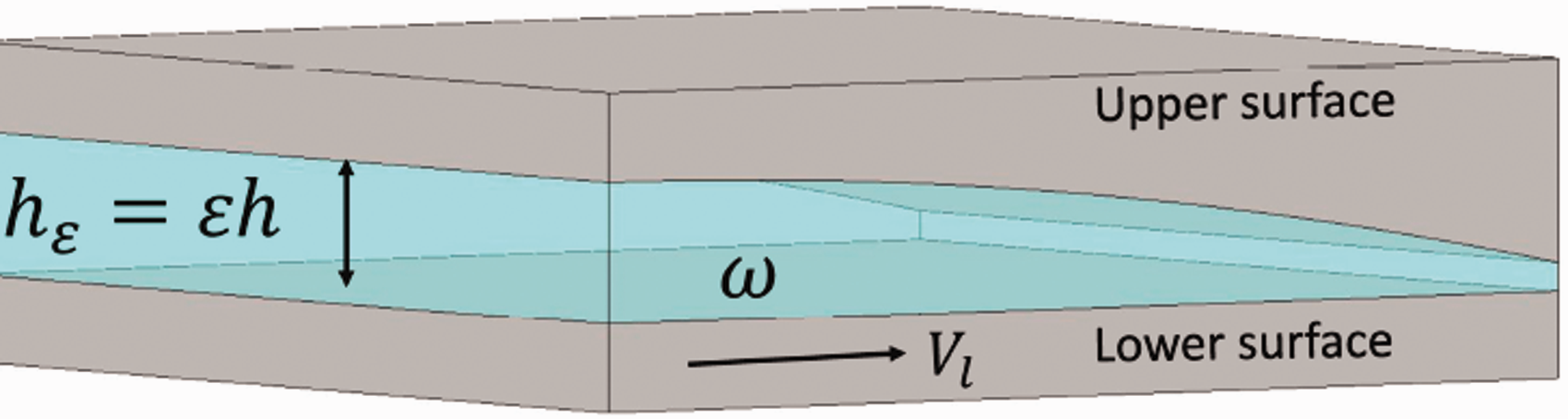
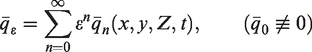
Let us consider flow in a thin domain between two surfaces which are in relative motion, see Figure 1. More precisely, we will study the case when the lower surface is in the xy-plane and consists of the points $(x,y,0)$ where $(x,y)\in \omega \in {ℝ}^2$ and the upper surface is $\left\{(x,y,z):z=\epsilon h(x,y,t),\epsilon >0\right\}$ , where $h(x,y,t)$ is a strictly positive smooth function which is defined for $(x,y)\in \omega$ and times t > 0. This means that the fluid domain is

$${\Omega }_{\epsilon }(t)=\left\{(x,y,z)\in {ℝ}^3:(x,y)\in \omega \subset {ℝ}^2,0<z<\epsilon h(x,y,t),t>0\right\},$$

Figure 1.

Illustration of the fluid domain ${\Omega }_{\epsilon }(t)$ between two surfaces in relative motion.

see Figure 1. Moreover, we define

$$Q_{\epsilon }=\left\{(x,y,z,t):(x,y,z)\in {\Omega }_{\epsilon }(t),0<t<T\right\}.$$

The physical interpretation is that h describes the shape of the upper surface and ε is a small parameter which is related to the distance $h_{\epsilon }$ between the surfaces, i.e. the film thickness). We will study the situation when the lower surface is moving in the xy-plane with the velocity $V_l=(u_l,v_l,0)$ and the upper surface ( $z=\epsilon h(x,y,t)$ ) is only moving in the z-direction with the velocity $V_u=(0,0,w_u)$ . We assume no slip boundary conditions at both surfaces. The fluid is assumed to be incompressible and piezo-viscous. Moreover, we also assume that there is a body force $\mathbf{g}=(g_x,g_y,g_z)$ acting per unit mass.

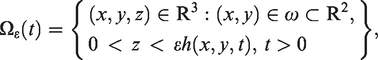
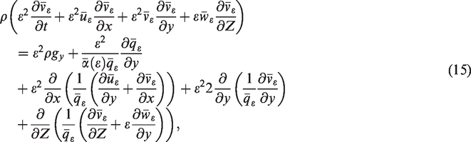
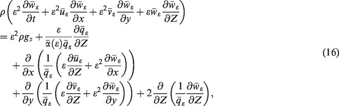
We showed in Part A that by using an implicit constitutive theory it is possible to formulate a generalisation of the Navier-Stokes equation which describes the velocity ${\mathbf{v}}_{\epsilon }=(u_{\epsilon },v_{\epsilon },w_{\epsilon })$ of the fluid and the pressure $p_{\epsilon }$ in the fluid. More precisely, we showed that

$$\begin{array}{l}\rho \left(\frac{\partial {\mathbf{v}}_{\epsilon }}{\partial t}+\left({\mathbf{v}}_{\epsilon }·\nabla \right){\mathbf{v}}_{\epsilon }\right)=\rho \mathbf{g}-\nabla p_{\epsilon }\\ +\text{div}\left[\mu (p_{\epsilon })\left(\nabla {\mathbf{v}}_{\epsilon }+{(\nabla {\mathbf{v}}_{\epsilon })}^T\right)\right],\text{in} Q_{\epsilon }\hspace{0.17em},\end{array}$$

(3)

where ρ is the constant density of the fluid and $\mu (p_{\epsilon })$ is a given viscosity-pressure relation. As usual, the Navier-Stokes equation is always solved together with the equation for the conservation of mass. For an incompressible fluid it is reduced to that the flow must be isochoric, i.e.

$$\text{div}{\mathbf{v}}_{\epsilon }=0,\text{in} Q_{\epsilon }.$$

(4)

To have a well-defined problem, we have to specify a viscosity-pressure relation. One choice is the constitutive relationship, which is frequently referred to as Barus’ law. ^b It is an exponential consitutive relationship between the viscosity and the pressure, which states that

$$\mu (p_{\epsilon })={\mu }_a{e}^{\alpha (p_{\epsilon }-p_a)},$$

(5)

where p_a represents ambient pressure, μ_a is the viscosity when $p_{\epsilon }=p_a$ and α a fluid viscosity-pressure coefficient.

When the fluid film is very thin, then it is difficult to compute the solution $({\mathbf{v}}_{\epsilon },p_{\epsilon })$ to the system (3) and (4) with present day computers. Therefore, it is important to find a way to simplify this system of equations, but of course in such a way that they still describe the flow sufficiently accurately. In this paper, we will present a new method for simplifying the system of equations (3) and (4), when the lubricant film thickness is much smaller than the size of the surfaces, i.e. for small values of ε. As we will see the result depends on the size of viscosity-pressure coefficient α. Our strategy is to let $\epsilon \to 0$ and see if we can obtain a limit problem which may be used as a lower-dimensional model for the flow. In particular, we are interested in justifying (2) by using this strategy, which is described in Section A strategy for finding a lower-dimensional model for the flow.

In the following, we will present two slightly different approaches. In the first one, described in Section A lower-dimensional equation for the pressure: First a change of variables and thereafter asymptotic analysis as $\mathit{\epsilon }\to \mathbf{0}$ , we start by carrying out a change of variables in the balance of linear momentum (3). This transformation is similar to the one that Muskat and Evinger introduced in literature, ⁴ in order to linearise the generalised Reynolds equation (2), see also the work by Ertel. ⁵ For more recent work discussing this transformation in connection to (2) and not the balance of linear momentum (3), see e.g. literature.^6,7 Then we scale the transformed equation to be able to pass to the limit as $\epsilon \to 0$ . Finally, by virtue of the change of variables, we are able to use the limit problem to derive a linear equation for the transformed pressure. In the second approach, which is outlined in Section A lower-dimensional equation for the pressure: First asymptotic analysis as $\mathit{\epsilon }\to \mathbf{0}$ and thereafter a change of variables, we start by scaling the equation (3) so that we can pass to the limit as $\epsilon \to 0$ . Then we use the limit problem to derive the nonlinear generalised Reynolds equation (2), which we thereafter linearise by means of a change of variables.

Let us discuss the change of variables that we will use in the first approach. Indeed, let F be the function such that $F(p_{\epsilon })=1/\mu (p_{\epsilon })$ , where $\mu (p_{\epsilon })$ is the viscosity-pressure relation (5) and define f as the function such that $F^{\prime }(p_{\epsilon })=f(p_{\epsilon })$ . We define the new variable

$$q_{\epsilon }=F(p_{\epsilon })=\frac{1}{{\mu }_a{e}^{\alpha (p_{\epsilon }-p_a)}}$$

(6)

and observe that

$$\begin{array}{l}\nabla q_{\epsilon }=F^{\prime }(p_{\epsilon })\nabla p_{\epsilon }=f(p_{\epsilon })\nabla p_{\epsilon }\\ =f\left(F^{-1}(q_{\epsilon })\right)\nabla p_{\epsilon }=\text{-}\alpha q_{\epsilon }\nabla p_{\epsilon }\hspace{0.17em},\end{array}$$

(7)

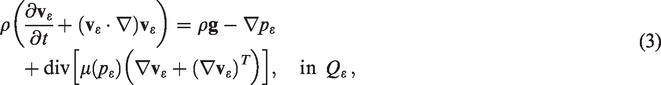
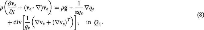
By using (7) we can replace $\nabla p_{\epsilon }$ in the equation (3) with $\text{-}{(\alpha q_{\epsilon })}^{\text{-}1}\nabla q_{\epsilon }$ and we obtain

$$\begin{array}{l}\rho \left(\frac{\partial {\mathbf{v}}_{\epsilon }}{\partial t}+\left({\mathbf{v}}_{\epsilon }·\nabla \right){\mathbf{v}}_{\epsilon }\right)=\rho \mathbf{g}+\frac{1}{\alpha q_{\epsilon }}\nabla q_{\epsilon }\\ +\text{div}\left[\frac{1}{q_{\epsilon }}\left(\nabla {\mathbf{v}}_{\epsilon }+{(\nabla {\mathbf{v}}_{\epsilon })}^T\right)\right],\text{in} Q_{\epsilon }\hspace{0.17em}.\end{array}$$

(8)

It should be noted that the μ_a does not appear explicitly in (8). When the solution $({\mathbf{v}}_{\epsilon },q_{\epsilon })$ of the system (8) and (4) has been computed, then we can use (6) to find the solution $({\mathbf{v}}_{\epsilon },p_{\epsilon })$ of the original system (3) and (4).

A strategy for finding a lower-dimensional model for the flow

Assume that for a given ${\epsilon }^{\prime }\ll 1$ we want to compute the solution $({\mathbf{v}}_{{\epsilon }^{\prime }},p_{{\epsilon }^{\prime }})$ to the system (3) and (4) with the viscosity-pressure relation (5). One approach is of course to try to solve the system numerically. However, this is difficult even with today’s computers and software. Therefore, we try to simplify the system of equations and thereafter solve the simplified system. The problem is how to simplify the system so that its solution is a good approximation of the solution to the original one. We will now present one strategy for how this can be done.

Use the change of variables (6) to transform the equation (3) into (8), with solution $({\mathbf{v}}_{{\epsilon }^{\prime }},q_{{\epsilon }^{\prime }})$ .

Construct a sequence ${\{({\overline{\mathbf{v}}}_{\epsilon },{\overline{q}}_{\epsilon })\}}_{\epsilon \in {ℝ}_{+}}$ so that $({\overline{\mathbf{v}}}_{{\epsilon }^{\prime }},{\overline{q}}_{{\epsilon }^{\prime }})$ coincides with the sought solution $({\mathbf{v}}_{{\epsilon }^{\prime }},q_{{\epsilon }^{\prime }})$ for $\epsilon =\epsilon \prime$ , i.e. $({\overline{\mathbf{v}}}_{{\epsilon }^{\prime }},{\overline{q}}_{{\epsilon }^{\prime }})=({\mathbf{v}}_{{\epsilon }^{\prime }},q_{{\epsilon }^{\prime }})$ .

Show that ${\overline{\mathbf{v}}}_{\epsilon }\to {\overline{\mathbf{v}}}_0$ and ${\overline{q}}_{\epsilon }\to {\overline{q}}_0$ , as $\epsilon \to 0,$ where $({\overline{\mathbf{v}}}_0,{\overline{q}}_0)$ is the solution of some limit problem.

Use that ${\epsilon }^{\prime }\ll 1$ to approximate $({\mathbf{v}}_{{\epsilon }^{\prime }},q_{{\epsilon }^{\prime }})$ with the solution $({\overline{\mathbf{v}}}_0,{\overline{q}}_0)$ to the limit problem, i.e. ${\mathbf{v}}_{{\epsilon }^{\prime }}={\overline{\mathbf{v}}}_{{\epsilon }^{\prime }}\approx {\overline{\mathbf{v}}}_0$ and $q_{{\epsilon }^{\prime }}={\overline{q}}_{{\epsilon }^{\prime }}\approx {\overline{q}}_0$ .

Use (6) to obtain an approximation of $p_{{\epsilon }^{\prime }}$ .

The question now is how to construct the sequence $\{({\overline{\mathbf{v}}}_{\epsilon },{\overline{q}}_{\epsilon })\}$ . The natural choice is $\{({\overline{\mathbf{v}}}_{\epsilon },{\overline{q}}_{\epsilon })\}=\{({\mathbf{v}}_{\epsilon },q_{\epsilon })\}$ , but this is not possible. This is realised by discussing as follows: from a physical point of view it is clear that if the velocity of the lower surface is kept constant, then pressure $p_{\epsilon }$ will go to infinity as $\epsilon \to 0$ . This together with (6) implies that $q_{\epsilon }\to q_0$ , where $q_0=0$ , and we can not use $q_0=0$ to find a useful approximation for $p_{{\epsilon }^{\prime }}$ . Thus we must find another choice, where $\left\{{\overline{q}}_{\epsilon }\right\}$ has a nonzero limit. To obtain this limit we will decrease the viscosity-pressure coefficient α simultaneously as ε goes to zero. The problem is, if we can find a proper scaling of α, i.e. can we describe how α should decrease as $\epsilon \to 0$ in order to get a useful nonzero limit ${\overline{q}}_0$ . In next section we will discus this, derive a single lower-dimensional equation for ${\overline{q}}_0$ and show that if α is “small”, then we can find a good approximation of $p_{{\epsilon }^{\prime }}$ by solving equation (2).

A lower-dimensional equation for the pressure: First a change of variables and thereafter asymptotic analysis as $\mathit{\epsilon }\to \mathbf{0}$

In this following subsections, we will perform the sequence of steps in the strategy presented in Section A strategy for finding a lower-dimensional model for the flow.

Construction of the sequence $\left\{\left({\overline{\mathbf{v}}}_{\epsilon },{\overline{q}}_{\epsilon }\right)\right\}$

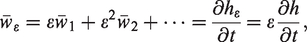
Let us construct a sequence $\{({\overline{\mathbf{v}}}_{\epsilon },{\overline{q}}_{\epsilon })\}$ such that $({\overline{\mathbf{v}}}_{{\epsilon }^{\prime }},{\overline{q}}_{{\epsilon }^{\prime }})=({\mathbf{v}}_{{\epsilon }^{\prime }},q_{{\epsilon }^{\prime }})$ , where $({\mathbf{v}}_{{\epsilon }^{\prime }},q_{{\epsilon }^{\prime }})$ is the solution of (8). We start by defining an auxiliary ε-dependent viscosity-pressure relation

$${\mu }_{\epsilon }(p_{\epsilon })={\mu }_a{e}^{\overline{\alpha }(\epsilon )(p_{\epsilon }-p_a)},$$

(9)

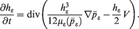
where the function $\overline{\alpha }$ is chosen such that $\overline{\alpha }({\epsilon }^{\prime })=\alpha$ , i.e. when $\epsilon ={\epsilon }^{\prime }$ the auxiliary viscosity-pressure relation (9) is the same as the physical viscosity-pressure relation (5). In terms of $({\overline{\mathbf{v}}}_{\epsilon },{\overline{p}}_{\epsilon })$ , the balance of linear momentum corresponding to the auxiliary viscosity-pressure relation (9) reads

$$\begin{array}{l}\rho \left(\frac{\partial {\overline{\mathbf{v}}}_{\epsilon }}{\partial t}+\left({\overline{\mathbf{v}}}_{\epsilon }·\nabla \right){\overline{\mathbf{v}}}_{\epsilon }\right)=\rho \mathbf{g}-\nabla {\overline{p}}_{\epsilon }\\ +\text{div}\left[{\mu }_{\epsilon }({\overline{p}}_{\epsilon })\left(\nabla {\overline{\mathbf{v}}}_{\epsilon }+{(\nabla {\overline{\mathbf{v}}}_{\epsilon })}^T\right)\right],\text{in} Q_{\epsilon }\hspace{0.17em},\end{array}$$

(10)

and the associated equation for the conservation of mass is

$$\text{div} {\overline{\mathbf{v}}}_{\epsilon }=0,\text{in} Q_{\epsilon }.$$

(11)

By carrying out the change of variables

$${\overline{q}}_{\epsilon }=\frac{1}{{\mu }_{\epsilon }({\overline{p}}_{\epsilon })}=\frac{1}{{\mu }_a{e}^{\overline{\alpha }(\epsilon )({\overline{p}}_{\epsilon }-p_a)}},$$

(12)

equation (10) becomes

$$\begin{array}{l}\rho \left(\frac{\partial {\overline{\mathbf{v}}}_{\epsilon }}{\partial t}+\left({\overline{\mathbf{v}}}_{\epsilon }·\nabla \right){\overline{\mathbf{v}}}_{\epsilon }\right)=\rho \mathbf{g}+\frac{1}{\overline{\alpha }(\epsilon ){\overline{q}}_{\epsilon }}\nabla {\overline{q}}_{\epsilon }\\ +\text{div}\left[\frac{1}{{\overline{q}}_{\epsilon }}\left(\nabla {\overline{\mathbf{v}}}_{\epsilon }+{(\nabla {\overline{\mathbf{v}}}_{\epsilon })}^T\right)\right],\text{in} {\Omega }_{\epsilon }\hspace{0.17em}.\end{array}$$

(13)

The sequence of solutions $\{({\overline{\mathbf{v}}}_{\epsilon },{\overline{q}}_{\epsilon })\}$ to (13) satisfies the requirement that $({\overline{\mathbf{v}}}_{{\epsilon }^{\prime }},{\overline{q}}_{{\epsilon }^{\prime }})=({\mathbf{v}}_{{\epsilon }^{\prime }},q_{{\epsilon }^{\prime }})$ . It remains to determine how $\overline{\alpha }$ should be chosen to obtain a useful limit $({\overline{\mathbf{v}}}_0,{\overline{q}}_0)$ as $\epsilon \to 0$ .

Transformation to a fix domain through a change of variables

The first step in our asymptotic analysis as $\epsilon \to 0$ is to convert the ε-dependent domain $Q_{\epsilon }$ (non-cylindrical) into a fix domain Q (cylindrical). We do this by introducing the fast variable $Z=z/\epsilon$ . In the new variables $(x,y,Z,t)$ the domain becomes

$$Q=\left\{(x,y,Z,t):(x,y)\in \omega \subset {ℝ}^2,0<Z<h(x,y,t),t>0\right\}.$$

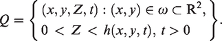
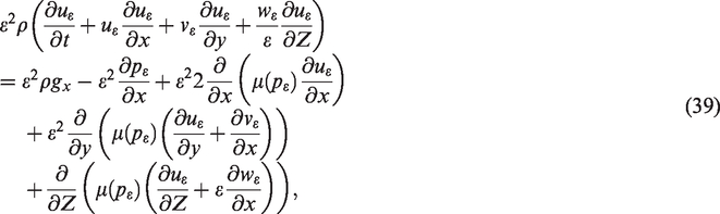
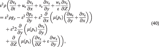
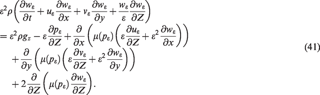
The equation (13) expressed in the fast variable Z should then be solved on the fixed domain Q, and in component form it reads

$$\begin{array}{l}\rho \left({\epsilon }^2\frac{\partial {\overline{u}}_{\epsilon }}{\partial t}+{\epsilon }^2{\overline{u}}_{\epsilon }\frac{\partial {\overline{u}}_{\epsilon }}{\partial x}+{\epsilon }^2{\overline{v}}_{\epsilon }\frac{\partial {\overline{u}}_{\epsilon }}{\partial y}+\epsilon {\overline{w}}_{\epsilon }\frac{\partial {\overline{u}}_{\epsilon }}{\partial Z}\right)\\ ={\epsilon }^2\rho g_x+\frac{{\epsilon }^2}{\overline{\alpha }(\epsilon ){\overline{q}}_{\epsilon }}\frac{\partial {\overline{q}}_{\epsilon }}{\partial x}+{\epsilon }^{2}2\frac{\partial }{\partial x}\left(\frac{1}{{\overline{q}}_{\epsilon }}\frac{\partial {\overline{u}}_{\epsilon }}{\partial x}\right)\\ +{\epsilon }^2\frac{\partial }{\partial y}\left(\frac{1}{{\overline{q}}_{\epsilon }}\left(\frac{\partial {\overline{u}}_{\epsilon }}{\partial y}+\frac{\partial {\overline{v}}_{\epsilon }}{\partial x}\right)\right)\\ +\frac{\partial }{\partial Z}\left(\frac{1}{{\overline{q}}_{\epsilon }}\left(\frac{\partial {\overline{u}}_{\epsilon }}{\partial Z}+\epsilon \frac{\partial {\overline{w}}_{\epsilon }}{\partial x}\right)\right),\end{array}$$

(14)

$$\begin{array}{l}\rho \left({\epsilon }^2\frac{\partial {\overline{v}}_{\epsilon }}{\partial t}+{\epsilon }^2{\overline{u}}_{\epsilon }\frac{\partial {\overline{v}}_{\epsilon }}{\partial x}+{\epsilon }^2{\overline{v}}_{\epsilon }\frac{\partial {\overline{v}}_{\epsilon }}{\partial y}+\epsilon {\overline{w}}_{\epsilon }\frac{\partial {\overline{v}}_{\epsilon }}{\partial Z}\right)\\ ={\epsilon }^2\rho g_y+\frac{{\epsilon }^2}{\overline{\alpha }(\epsilon ){\overline{q}}_{\epsilon }}\frac{\partial {\overline{q}}_{\epsilon }}{\partial y}\\ +{\epsilon }^2\frac{\partial }{\partial x}\left(\frac{1}{{\overline{q}}_{\epsilon }}\left(\frac{\partial {\overline{u}}_{\epsilon }}{\partial y}+\frac{\partial {\overline{v}}_{\epsilon }}{\partial x}\right)\right)+{\epsilon }^{2}2\frac{\partial }{\partial y}\left(\frac{1}{{\overline{q}}_{\epsilon }}\frac{\partial {\overline{v}}_{\epsilon }}{\partial y}\right)\\ +\frac{\partial }{\partial Z}\left(\frac{1}{{\overline{q}}_{\epsilon }}\left(\frac{\partial {\overline{v}}_{\epsilon }}{\partial Z}+\epsilon \frac{\partial {\overline{w}}_{\epsilon }}{\partial y}\right)\right),\end{array}$$

(15)

$$\begin{array}{l}\rho \left({\epsilon }^2\frac{\partial {\overline{w}}_{\epsilon }}{\partial t}+{\epsilon }^2{\overline{u}}_{\epsilon }\frac{\partial {\overline{w}}_{\epsilon }}{\partial x}+{\epsilon }^2{\overline{v}}_{\epsilon }\frac{\partial {\overline{w}}_{\epsilon }}{\partial y}+\epsilon {\overline{w}}_{\epsilon }\frac{\partial {\overline{w}}_{\epsilon }}{\partial Z}\right)\\ ={\epsilon }^2\rho g_z+\frac{\epsilon }{\overline{\alpha }(\epsilon ){\overline{q}}_{\epsilon }}\frac{\partial {\overline{q}}_{\epsilon }}{\partial Z}\\ +\frac{\partial }{\partial x}\left(\frac{1}{{\overline{q}}_{\epsilon }}\left(\epsilon \frac{\partial {\overline{u}}_{\epsilon }}{\partial Z}+{\epsilon }^2\frac{\partial {\overline{w}}_{\epsilon }}{\partial x}\right)\right)\\ +\frac{\partial }{\partial y}\left(\frac{1}{{\overline{q}}_{\epsilon }}\left(\epsilon \frac{\partial {\overline{v}}_{\epsilon }}{\partial Z}+{\epsilon }^2\frac{\partial {\overline{w}}_{\epsilon }}{\partial y}\right)\right)+2\frac{\partial }{\partial Z}\left(\frac{1}{{\overline{q}}_{\epsilon }}\frac{\partial {\overline{w}}_{\epsilon }}{\partial Z}\right),\end{array}$$

(16)

after multiplication with ${\epsilon }^2$ . The equation for conservation of mass expressed in the fast variable becomes

$$\epsilon \frac{\partial {\overline{u}}_{\epsilon }}{\partial x}+\epsilon \frac{\partial {\overline{v}}_{\epsilon }}{\partial y}+\frac{\partial {\overline{w}}_{\epsilon }}{\partial Z}=0\text{in} Q.$$

(17)

Expansion of the velocity field and consequences of the incompressibility condition

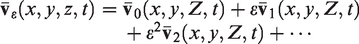
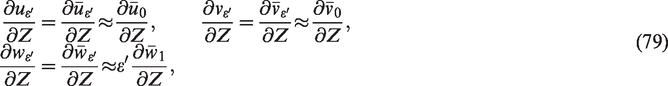
Let us assume that ${\overline{\mathbf{v}}}_{\epsilon }=({\overline{u}}_{\epsilon }$ , ${\overline{v}}_{\epsilon },{\overline{w}}_{\epsilon })$ can be expressed as a power series in the small variable ε. Indeed,

$$\begin{array}{l}{\overline{\mathbf{v}}}_{\epsilon }(x,y,z,t)={\overline{\mathbf{v}}}_0(x,y,Z,t)+\epsilon {\overline{\mathbf{v}}}_1(x,y,Z,t)\\ +{\epsilon }^2{\overline{\mathbf{v}}}_2(x,y,Z,t)+\cdots \end{array}$$

or in component form

$$\begin{array}{l}{\overline{u}}_{\epsilon }(x,y,Z,t)={\overline{u}}_0(x,y,Z,t)+\epsilon {\overline{u}}_1(x,y,Z,t)\\ +{\epsilon }^2{\overline{u}}_2(x,y,Z,t)+\cdots ,\end{array}$$

(18)

$$\begin{array}{l}{\overline{v}}_{\epsilon }(x,y,Z,t)={\overline{v}}_0(x,y,Z,t)+\epsilon {\overline{v}}_1(x,y,Z,t)\\ +{\epsilon }^2{\overline{v}}_2(x,y,Z,t)+\cdots ,\end{array}$$

(19)

$$\begin{array}{l}{\overline{w}}_{\epsilon }(x,y,Z,t)={\overline{w}}_0(x,y,Z,t)+\epsilon {\overline{w}}_1(x,y,Z,t)\\ +{\epsilon }^2{\overline{w}}_2(x,y,Z,t)+\cdots .\end{array}$$

(20)

The characteristic size of ${\overline{u}}_0$ and ${\overline{v}}_0$ is the same as the boundary condition, which motivates that the first term in expansions of ${\overline{u}}_{\epsilon }$ and ${\overline{v}}_{\epsilon }$ are of $\mathcal{O}(1)$ . Let us now determine the order of ${\overline{w}}_{\epsilon }$ by inserting the expansion of ${\overline{\mathbf{v}}}_{\epsilon }$ into the scaled incompressibility condition (17) and comparing terms of the same order of ε. This leads to that (we only consider the two lowest orders)

$${\mathit{\epsilon }}^0:\frac{\partial {\overline{w}}_0}{\partial Z}=0,$$

(21)

$${\mathit{\epsilon }}^1:\frac{\partial {\overline{u}}_0}{\partial x}+\frac{\partial {\overline{v}}_0}{\partial y}+\frac{\partial {\overline{w}}_1}{\partial Z}=0.$$

(22)

From (21) and the boundary condition ${\overline{w}}_0(x,y,0,t)=0$ it follows that

$${\overline{w}}_0=0.$$

The no-slip boundary condition on the upper surface implies that at the upper surface

$${\overline{w}}_{\epsilon }=\epsilon {\overline{w}}_1+{\epsilon }^2{\overline{w}}_2+\cdots =\frac{\partial h_{\epsilon }}{\partial t}=\epsilon \frac{\partial h}{\partial t},$$

and at the lower surface ${\overline{w}}_1=0,$ i.e.

$${\overline{w}}_1(x,y,h(x,y,t),t)=\frac{\partial h}{\partial t}(x,y,t)\text{ and } {\overline{w}}_1(x,y,0,t)=0.$$

(23)

Thus, ${\overline{w}}_{\epsilon }$ is of order $\mathcal{O}(\epsilon )$ .

A lower-dimensional equation for approximating ${\mathit{q}}_{\mathit{\epsilon }}$

As described above $\overline{\alpha }$ must decrease as $\epsilon \to 0$ in order to have a nonzero limit. We start by trying

$$\overline{\alpha }=\overline{\alpha }(\epsilon )=\beta {\epsilon }^k,k>0,\beta >0.$$

(24)

The question is then what k should be in order for ${\overline{q}}_{\epsilon }$ to have an expansion of the form

$${\overline{q}}_{\epsilon }={\displaystyle \sum _{n=0}^{\infty }{\epsilon }^n}{\overline{q}}_n(x,y,Z,t),({\overline{q}}_0\cancel{\equiv }0)$$

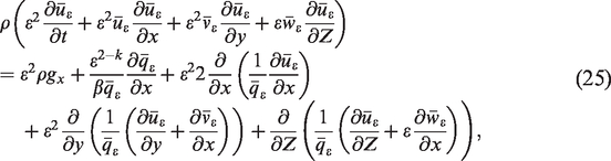
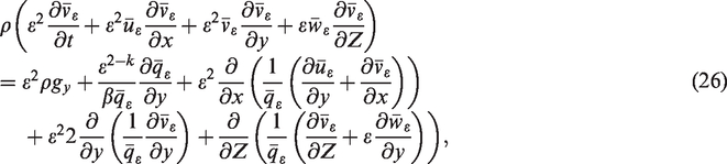
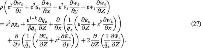
In order to see this we first insert (24) into (14)-(16) and obtain

$$\begin{array}{l}\rho \left({\epsilon }^2\frac{\partial {\overline{u}}_{\epsilon }}{\partial t}+{\epsilon }^2{\overline{u}}_{\epsilon }\frac{\partial {\overline{u}}_{\epsilon }}{\partial x}+{\epsilon }^2{\overline{v}}_{\epsilon }\frac{\partial {\overline{u}}_{\epsilon }}{\partial y}+\epsilon {\overline{w}}_{\epsilon }\frac{\partial {\overline{u}}_{\epsilon }}{\partial Z}\right)\\ ={\epsilon }^2\rho g_x+\frac{{\epsilon }^{2-k}}{\beta {\overline{q}}_{\epsilon }}\frac{\partial {\overline{q}}_{\epsilon }}{\partial x}+{\epsilon }^{2}2\frac{\partial }{\partial x}\left(\frac{1}{{\overline{q}}_{\epsilon }}\frac{\partial {\overline{u}}_{\epsilon }}{\partial x}\right)\\ +{\epsilon }^2\frac{\partial }{\partial y}\left(\frac{1}{{\overline{q}}_{\epsilon }}\left(\frac{\partial {\overline{u}}_{\epsilon }}{\partial y}+\frac{\partial {\overline{v}}_{\epsilon }}{\partial x}\right)\right)+\frac{\partial }{\partial Z}\left(\frac{1}{{\overline{q}}_{\epsilon }}\left(\frac{\partial {\overline{u}}_{\epsilon }}{\partial Z}+\epsilon \frac{\partial {\overline{w}}_{\epsilon }}{\partial x}\right)\right),\end{array}$$

(25)

$$\begin{array}{l}\rho \left({\epsilon }^2\frac{\partial {\overline{v}}_{\epsilon }}{\partial t}+{\epsilon }^2{\overline{u}}_{\epsilon }\frac{\partial {\overline{v}}_{\epsilon }}{\partial x}+{\epsilon }^2{\overline{v}}_{\epsilon }\frac{\partial {\overline{v}}_{\epsilon }}{\partial y}+\epsilon {\overline{w}}_{\epsilon }\frac{\partial {\overline{v}}_{\epsilon }}{\partial Z}\right)\\ ={\epsilon }^2\rho g_y+\frac{{\epsilon }^{2-k}}{\beta {\overline{q}}_{\epsilon }}\frac{\partial {\overline{q}}_{\epsilon }}{\partial y}+{\epsilon }^2\frac{\partial }{\partial x}\left(\frac{1}{{\overline{q}}_{\epsilon }}\left(\frac{\partial {\overline{u}}_{\epsilon }}{\partial y}+\frac{\partial {\overline{v}}_{\epsilon }}{\partial x}\right)\right)\\ +{\epsilon }^{2}2\frac{\partial }{\partial y}\left(\frac{1}{{\overline{q}}_{\epsilon }}\frac{\partial {\overline{v}}_{\epsilon }}{\partial y}\right)+\frac{\partial }{\partial Z}\left(\frac{1}{{\overline{q}}_{\epsilon }}\left(\frac{\partial {\overline{v}}_{\epsilon }}{\partial Z}+\epsilon \frac{\partial {\overline{w}}_{\epsilon }}{\partial y}\right)\right),\end{array}$$

(26)

$$\begin{array}{l}\rho \left({\epsilon }^2\frac{\partial {\overline{w}}_{\epsilon }}{\partial t}+{\epsilon }^2{\overline{u}}_{\epsilon }\frac{\partial {\overline{w}}_{\epsilon }}{\partial x}+{\epsilon }^2{\overline{v}}_{\epsilon }\frac{\partial {\overline{w}}_{\epsilon }}{\partial y}+\epsilon {\overline{w}}_{\epsilon }\frac{\partial {\overline{w}}_{\epsilon }}{\partial Z}\right)\\ ={\epsilon }^2\rho g_z+\frac{{\epsilon }^{1-k}}{\beta {\overline{q}}_{\epsilon }}\frac{\partial {\overline{q}}_{\epsilon }}{\partial Z}+\frac{\partial }{\partial x}\left(\frac{1}{{\overline{q}}_{\epsilon }}\left(\epsilon \frac{\partial {\overline{u}}_{\epsilon }}{\partial Z}+{\epsilon }^2\frac{\partial {\overline{w}}_{\epsilon }}{\partial x}\right)\right)\\ +\frac{\partial }{\partial y}\left(\frac{1}{{\overline{q}}_{\epsilon }}\left(\epsilon \frac{\partial {\overline{v}}_{\epsilon }}{\partial Z}+{\epsilon }^2\frac{\partial {\overline{w}}_{\epsilon }}{\partial y}\right)\right)+2\frac{\partial }{\partial Z}\left(\frac{1}{{\overline{q}}_{\epsilon }}\frac{\partial {\overline{w}}_{\epsilon }}{\partial Z}\right).\end{array}$$

(27)

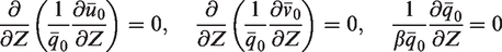
Let us now insert the expansions of ${\overline{\mathbf{v}}}_{\epsilon }$ and ${\overline{q}}_{\epsilon }$ into (25)-(27) in order to see what system of equations we will have for the dominating terms. We have three different cases (recall that ${\overline{w}}_{\epsilon }=\mathcal{O}(\epsilon )$ ):

$$0<\mathbf{k}<2\mathbf{:}$$

$$\frac{\partial }{\partial Z}\left(\frac{1}{{\overline{q}}_0}\frac{\partial {\overline{u}}_0}{\partial Z}\right)=0,\frac{\partial }{\partial Z}\left(\frac{1}{{\overline{q}}_0}\frac{\partial {\overline{v}}_0}{\partial Z}\right)=0,\frac{1}{\beta {\overline{q}}_0}\frac{\partial {\overline{q}}_0}{\partial Z}=0$$

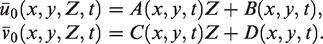
From the third equation it follows that ${\overline{q}}_0$ does not depend on Z, i.e. ${\overline{q}}_0={\overline{q}}_0(x,y,t)$ . This means that the first two equations may be integrated twice with respect to Z and we obtain that ${\overline{u}}_0$ and ${\overline{v}}_0$ are of the form

$$\begin{array}{l}{\overline{u}}_0(x,y,Z,t)=A(x,y,t)Z+B(x,y,t),\\ {\overline{v}}_0(x,y,Z,t)=C(x,y,t)Z+D(x,y,t).\end{array}$$

where A, B, C and D are functions appearing in the integration. Hence only Couette flow, is considered in the limit problem which is unrealistic if the surfaces are not parallel. We draw the conclusion that the case $0<k<2$ is uninteresting.

$$\mathbf{k}>\mathbf{2}\mathbf{:}$$

$$\frac{1}{\beta q_0}\frac{\partial q_0}{\partial x}=0,\frac{1}{\beta q_0}\frac{\partial q_0}{\partial y}=0,\frac{1}{\beta q_0}\frac{\partial q_0}{\partial Z}=0.$$

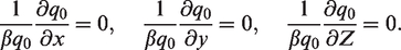
That ${\overline{q}}_0$ does not depend on Z is what we require from a dimension reduced model. However, that ${\overline{q}}_0$ does not depend on neither x nor y if the surfaces are not parallel is not realistic and we conclude that the case k > 2 is uninteresting.

$$\mathbf{k}=\mathbf{2}\mathbf{:}$$

$$\frac{1}{\beta {\overline{q}}_0}\frac{\partial {\overline{q}}_0}{\partial x}+\frac{\partial }{\partial Z}\left(\frac{1}{{\overline{q}}_0}\frac{\partial {\overline{u}}_0}{\partial Z}\right)=0,$$

(28)

$$\frac{1}{\beta {\overline{q}}_0}\frac{\partial {\overline{q}}_0}{\partial y}+\frac{\partial }{\partial Z}\left(\frac{1}{{\overline{q}}_0}\frac{\partial {\overline{v}}_0}{\partial Z}\right)=0,$$

(29)

$$\frac{1}{\beta {\overline{q}}_0}\frac{\partial {\overline{q}}_0}{\partial Z}=0.$$

(30)

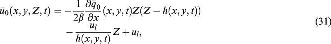
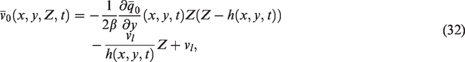
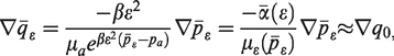
From this system we can derive a Reynold type equation for q₀ by using similar arguments as in the derivation of the classical Reynolds equation. For the readers convenience we present the details. Indeed, from (30) we see that ${\overline{q}}_0$ does not depend on Z, i.e. ${\overline{q}}_0={\overline{q}}_0(x,y,t)$ . This makes it possible to integrate (28) and (29) twice with respect to Z and we obtain

$$\begin{array}{l}{\overline{u}}_0(x,y,Z,t)=-\frac{1}{2\beta }\frac{\partial {\overline{q}}_0}{\partial x}(x,y,t)Z(Z-h(x,y,t))\\ -\frac{u_l}{h(x,y,t)}Z+u_l,\end{array}$$

(31)

$$\begin{array}{l}{\overline{v}}_0(x,y,Z,t)=-\frac{1}{2\beta }\frac{\partial {\overline{q}}_0}{\partial y}(x,y,t)Z(Z-h(x,y,t))\\ -\frac{v_l}{h(x,y,t)}Z+v_l,\end{array}$$

(32)

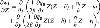
after applying no-slip boundary conditions stating that ${\overline{\mathbf{v}}}_{\mathbf{\epsilon }}=V_l=(u_l,v_l,0)$ at the lower surface and ${\overline{\mathbf{v}}}_{\mathbf{\epsilon }}=V_u=(0,0,w_u)$ at the upper surface. By inserting the expressions for ${\overline{u}}_0$ and ${\overline{v}}_0$ into the equation for conservation of mass (22) we obtain

$$\begin{array}{l}\frac{\partial {\overline{w}}_1}{\partial Z}=\frac{\partial }{\partial x}\left(\frac{1}{2\beta }\frac{\partial {\overline{q}}_0}{\partial x}Z(Z-h)+\frac{u_l}{h}Z-u_l\right)\\ +\frac{\partial }{\partial y}\left(\frac{1}{2\beta }\frac{\partial {\overline{q}}_0}{\partial y}Z(Z-h)+\frac{v_l}{h}Z-v_l\right).\end{array}$$

By integrating with respect to Z from 0 to h we can eliminate ${\overline{w}}_1$ . Indeed

$$\begin{array}{l}{\overline{w}}_1(x,y,h,t)-{\overline{w}}_1(x,y,0,t)\\ =\frac{\partial }{\partial x}{\displaystyle {\int }_0^h\frac{1}{2\beta }}\frac{\partial {\overline{q}}_0}{\partial x}Z(Z-h)+\frac{u_l}{h}Z-u_l\text{d}Z\\ +\frac{\partial }{\partial y}{\displaystyle {\int }_0^h\frac{1}{2\beta }}\frac{\partial {\overline{q}}_0}{\partial y}Z(Z-h)+\frac{v_l}{h}Z-v_l\text{d}Z\\ =-\frac{\partial }{\partial x}\left(\frac{h^3}{12\beta }\frac{\partial {\overline{q}}_0}{\partial x}+\frac{h{u}_l}{2}\right)-\frac{\partial }{\partial y}\left(\frac{h^3}{12\beta }\frac{\partial {\overline{q}}_0}{\partial y}+\frac{h{v}_l}{2}\right).\end{array}$$

(33)

This together with the boundary conditions (23) on ${\overline{w}}_1$ give the following lower-dimensional equation for ${\overline{q}}_0$ , the leading term in the expansion for ${\overline{q}}_{\epsilon }$ ,

$$\frac{\partial h}{\partial t}=-\text{div}\left(\frac{h^3}{12\beta }\nabla {\overline{q}}_0+\frac{h}{2}V\right),$$

(34)

where V is the two-dimensional vector $u_l\mathbf{i}+v_l\mathbf{j}$ .

Computing the pressure via inverse transformation

For small values of ε we have that ${\overline{q}}_{\epsilon }\approx {\overline{q}}_0$ . If we let ${\overline{p}}_{\epsilon }$ denote the pressure corresponding to ${\overline{q}}_{\epsilon }$ , then according to (12) we have that

$${\overline{q}}_{\epsilon }(x,y,Z,t)=\frac{1}{{\mu }_a{e}^{\beta {\epsilon }^2({\overline{p}}_{\epsilon }-p_a)}}\approx {\overline{q}}_0(x,y,t).$$

(35)

Solving for the pressure gives yields

$${\overline{p}}_{\epsilon }\approx p_a-\frac{1}{\beta {\epsilon }^2}\ln \left({\mu }_a{\overline{q}}_0\right).$$

In particular, we find that an approximation of $p_{{\epsilon }^{\prime }}$ , which we were after, may be obtained as

$$p_{{\epsilon }^{\prime }}={\overline{p}}_{{\epsilon }^{\prime }}\approx p_a-\frac{1}{\beta {\left({\epsilon }^{\prime }\right)}^2}\ln \left({\mu }_a{\overline{q}}_0\right)=p_a-\frac{1}{\alpha }\ln \left({\mu }_a{\overline{q}}_0\right).$$

(36)

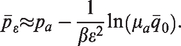
It can be noted that ${\overline{p}}_{\epsilon }=O({\epsilon }^{\text{-}2})$ for a fixed β.

The equation (34) can be expressed in terms of the physical distance between the surfaces, $h_{\epsilon }=\epsilon h$ . Indeed

$$\frac{\partial h_{\epsilon }}{\partial t}=-\text{div}\left(\frac{h_{\epsilon }^3}{12\overline{\alpha }(\epsilon )}\nabla {\overline{q}}_0+\frac{h_{\epsilon }}{2}V\right),$$

(37)

where $\overline{\alpha }(\epsilon )=\beta {\epsilon }^2$ . Moreover, from (35) we have the following approximation

$$\nabla {\overline{q}}_{\epsilon }=\frac{\text{-}\beta {\epsilon }^2}{{\mu }_a{e}^{\beta {\epsilon }^2({\overline{p}}_{\epsilon }-p_a)}}\nabla {\overline{p}}_{\epsilon }=\frac{\text{-}\overline{\alpha }(\epsilon )}{{\mu }_{\epsilon }({\overline{p}}_{\epsilon })}\nabla {\overline{p}}_{\epsilon }\approx \nabla q0,$$

for small values of ε. This inserted into (37) leads to an approximation of ${\overline{p}}_{\epsilon }$ by solving the equation

$$\frac{\partial h_{\epsilon }}{\partial t}=\text{div}\left(\frac{h_{\epsilon }^3}{12{\mu }_{\epsilon }({\overline{p}}_{\epsilon })}\nabla {\overline{p}}_{\epsilon }-\frac{h_{\epsilon }}{2}V\right).$$

In particular, we obtain an approximation for the pressure $p_{{\epsilon }^{\prime }}$ , corresponding to the film thickness $h_{{\epsilon }^{\prime }}$ , by solving

$$\frac{\partial h_{{\epsilon }^{\prime }}}{\partial t}=\text{div}\left(\frac{h_{{\epsilon }^{\prime }}^3}{12{\mu }_{{\epsilon }^{\prime }}(p_{{\epsilon }^{\prime }})}\nabla p_{{\epsilon }^{\prime }}-\frac{h_{{\epsilon }^{\prime }}}{2}V\right),$$

(38)

which is identical to (2). From now on we will refer to this equation as the piezo-viscous Reynolds equation. Hence, we have motivated that (2) may be used when the viscosity-pressure relation is given by (5) and α is sufficiently small.

We have just seen that we can find an approximation for the pressure corresponding to the film thickness $h_{{\epsilon }^{\prime }}$ by solving the equation (38). Since (38) is nonlinear it is however, from a computational point of view, beneficial to instead compute ${\overline{q}}_0$ by solving the equation (34) and thereafter use (36) to find the pressure $p_{{\epsilon }^{\prime }}.$ Indeed, the pressure $p_{\epsilon \prime }$ can be computed by the following lower-dimensional algorithm, based on the solution of the lower-dimensional equation (34) for q₀:

For a specific application when α and ${\epsilon }^{\prime }$ are known, use these values to determine β.

Compute ${\overline{q}}_0$ by solving (34).

Use (36) to compute $p_{{\epsilon }^{\prime }}$ .

In Section Numerical examples illustrating the convergence, where some numerical illustrations are presented we will use this lower-dimensional algorithm for the pressure.

Remark.

If one wants to solve many problems, then (34) in general has to be solved many times (one time for each value of β). However, if we do the change of variables $\tilde{q}:={\overline{q}}_0/\beta$ , then the transformed equation for $\tilde{q}$ is independent β. When $\tilde{q}$ is computed it can be used to compute ${\overline{q}}_0$ via ${\overline{q}}_0=\beta \tilde{q}$ .

A lower-dimensional equation for the pressure: First asymptotic analysis as $\mathit{\epsilon }\to \mathbf{0}$ and thereafter a change of variables

In the previous section, we derived a lower-dimensional equation for the flow by first carrying out a change of variables in the generalised Navier-Stokes equation and thereafter studying the asymptotic behavior as $\epsilon \to 0$ . All the calculations were carried out under the assumption that the viscosity-pressure relation is the one described by Barus’ law. In this section, we will proceed the other way around, i.e. we will first do the asymptotic analysis of the generalised Navier-Stokes equation and thereafter do a change of variables to obtain a linear Reynolds type of equation which can be used to calculate the pressure. To show that our results are not only valid for fluids which can be modeled by Barus’ law we will in this section extend the analysis so it includes all common viscosity-pressure relations, by adopting the expression given in (42). For convenience, but without loss of generality we assume in this section assume that p_a = 0 in (5).

As before we introduce the fast variable $Z=z/\epsilon$ and the generalised Navier-Stokes equation (3) in component form becomes

$$\begin{array}{l}{\epsilon }^2\rho \left(\frac{\partial u_{\epsilon }}{\partial t}+u_{\epsilon }\frac{\partial u_{\epsilon }}{\partial x}+v_{\epsilon }\frac{\partial u_{\epsilon }}{\partial y}+\frac{w_{\epsilon }}{\epsilon }\frac{\partial u_{\epsilon }}{\partial Z}\right)\\ ={\epsilon }^2\rho g_x-{\epsilon }^2\frac{\partial p_{\epsilon }}{\partial x}+{\epsilon }^{2}2\frac{\partial }{\partial x}\left(\mu (p_{\epsilon })\frac{\partial u_{\epsilon }}{\partial x}\right)\\ +{\epsilon }^2\frac{\partial }{\partial y}\left(\mu (p_{\epsilon })\left(\frac{\partial u_{\epsilon }}{\partial y}+\frac{\partial v_{\epsilon }}{\partial x}\right)\right)\\ +\frac{\partial }{\partial Z}\left(\mu (p_{\epsilon })\left(\frac{\partial u_{\epsilon }}{\partial Z}+\epsilon \frac{\partial w_{\epsilon }}{\partial x}\right)\right),\end{array}$$

(39)

$$\begin{array}{l}{\epsilon }^2\rho \left(\frac{\partial v_{\epsilon }}{\partial t}+u_{\epsilon }\frac{\partial v_{\epsilon }}{\partial x}+v_{\epsilon }\frac{\partial v_{\epsilon }}{\partial y}+\frac{w_{\epsilon }}{\epsilon }\frac{\partial v_{\epsilon }}{\partial Z}\right)\\ ={\epsilon }^2\rho g_y-{\epsilon }^2\frac{\partial p_{\epsilon }}{\partial y}+{\epsilon }^2\frac{\partial }{\partial x}\left(\mu (p_{\epsilon })\left(\frac{\partial u_{\epsilon }}{\partial y}+\frac{\partial v_{\epsilon }}{\partial x}\right)\right)\\ +{\epsilon }^{2}2\frac{\partial }{\partial y}\left(\mu (p_{\epsilon })\frac{\partial v_{\epsilon }}{\partial y}\right)\\ +\frac{\partial }{\partial Z}\left(\mu (p_{\epsilon })\left(\frac{\partial v_{\epsilon }}{\partial Z}+\epsilon \frac{\partial w_{\epsilon }}{\partial y}\right)\right),\end{array}$$

(40)

$$\begin{array}{l}{\epsilon }^2\rho \left(\frac{\partial w_{\epsilon }}{\partial t}+u_{\epsilon }\frac{\partial w_{\epsilon }}{\partial x}+v_{\epsilon }\frac{\partial w_{\epsilon }}{\partial y}+\frac{w_{\epsilon }}{\epsilon }\frac{\partial w_{\epsilon }}{\partial Z}\right)\\ ={\epsilon }^2\rho g_z-\epsilon \frac{\partial p_{\epsilon }}{\partial Z}+\frac{\partial }{\partial x}\left(\mu (p_{\epsilon })\left(\epsilon \frac{\partial u_{\epsilon }}{\partial Z}+{\epsilon }^2\frac{\partial w_{\epsilon }}{\partial x}\right)\right)\\ +\frac{\partial }{\partial y}\left(\mu (p_{\epsilon })\left(\epsilon \frac{\partial v_{\epsilon }}{\partial Z}+{\epsilon }^2\frac{\partial w_{\epsilon }}{\partial y}\right)\right)\\ +2\frac{\partial }{\partial Z}\left(\mu (p_{\epsilon })\frac{\partial w_{\epsilon }}{\partial Z}\right).\end{array}$$

(41)

In Section A lower-dimensional equation for the pressure: First a change of variables and thereafter asymptotic analysis as $\mathit{\epsilon }\to \mathbf{0}$ we used the Barus viscosity-pressure relation (5) to avoid some technicalities. However, the results hold for all common viscosity-pressure relations. To show this we will now only assume that the viscosity-pressure relation is on the form

$$\mu (p)={\mu }_{a}r(\alpha p),$$

(42)

where r is a strictly positive smooth increasing function such that $r(0)=1,\alpha \ge 0$ is a viscosity-pressure coefficient and μ_a is the viscosity corresponding to p = 0. The class (42) includes most commonly used viscosity-pressure relations, e.g. the Barus viscosity-pressure relation (5), Roelands viscosity-pressure relation ⁸ and the case with constant viscosity (α = 0).

Assume that we want to solve the system (39) to (41) for $\epsilon =\epsilon \prime \ll 1$ . A direct numerical computation is difficult with present day computing facilities and therefore we want to derive a simplified system. We will now do this by studying the asymptotic behavior as $\epsilon \to 0$ in order to find a limit problem which can be used to find an approximation of the solution $({\mathbf{v}}_{\epsilon \prime },p_{\epsilon \prime })$ . It is though not possible to obtain a useful limit problem by just letting $\epsilon \to 0$ . The reason for this is that $p_{\epsilon }$ goes to infinity as $\epsilon \to 0$ , see the discussion in Section A strategy for finding a lower-dimensional model for the flow, and hence the limit can not be used to find an approximation of $p_{\epsilon \prime }$ . This motivates that we introduce the scaled pressure ${\overline{p}}_{\epsilon }={\epsilon }^m{p}_{\epsilon }$ , m > 0, such that ${\overline{p}}_{\epsilon }\to {\overline{p}}_0$ for some nontrivial ${\overline{p}}_0$ . Moreover, from the viscosity-pressure relation (42) we see that

$$\mu (p_{\epsilon })={\mu }_{a}r(\alpha p_{\epsilon })={\mu }_{a}r(\alpha {\overline{p}}_{\epsilon }/{\epsilon }^m)\to \infty \text{as}\epsilon \to 0.$$

This creates a problem when we want to pass to the limit in the system (39)-(41) and motivates us to scale α to avoid this. Indeed, we define $\overline{\alpha }(\epsilon )=\beta {\epsilon }^k$ , where $k\ge m$ and β is chosen such that $\overline{\alpha }({\epsilon }^{\prime })=\alpha$ . We also define the auxiliary viscosity-pressure relations

$${\overline{\mu }}_{\epsilon }({\overline{p}}_{\epsilon })={\mu }_{a}r(\beta {\epsilon }^{k-m}{\overline{p}}_{\epsilon }).$$

(43)

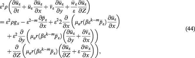
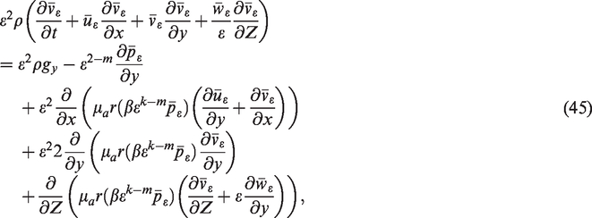
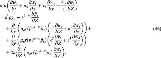
Note that ${\overline{\mu }}_{{\epsilon }^{\prime }}({\overline{p}}_{\epsilon \prime })=\mu (p_{\epsilon \prime })$ . By substituting $p_{\epsilon }$ with ${\epsilon }^{-m}{\overline{p}}_{\epsilon }$ and $\mu (p_{\epsilon })$ with ${\overline{\mu }}_{\epsilon }({\overline{p}}_{\epsilon })$ in (39) to (41) we obtain the system

$$\begin{array}{l}{\epsilon }^2\rho \left(\frac{\partial {\overline{u}}_{\epsilon }}{\partial t}+{\overline{u}}_{\epsilon }\frac{\partial {\overline{u}}_{\epsilon }}{\partial x}+{\overline{v}}_{\epsilon }\frac{\partial {\overline{u}}_{\epsilon }}{\partial y}+\frac{{\overline{w}}_{\epsilon }}{\epsilon }\frac{\partial {\overline{u}}_{\epsilon }}{\partial Z}\right)\\ ={\epsilon }^2\rho g_x-{\epsilon }^{2-m}\frac{\partial {\overline{p}}_{\epsilon }}{\partial x}+{\epsilon }^{2}2\frac{\partial }{\partial x}\left({\mu }_{a}r(\beta {\epsilon }^{k-m}{\overline{p}}_{\epsilon })\frac{\partial {\overline{u}}_{\epsilon }}{\partial x}\right)\\ +{\epsilon }^2\frac{\partial }{\partial y}\left({\mu }_{a}r(\beta {\epsilon }^{k-m}{\overline{p}}_{\epsilon })\left(\frac{\partial {\overline{u}}_{\epsilon }}{\partial y}+\frac{\partial {\overline{v}}_{\epsilon }}{\partial x}\right)\right)\\ +\frac{\partial }{\partial Z}\left({\mu }_{a}r(\beta {\epsilon }^{k-m}{\overline{p}}_{\epsilon })\left(\frac{\partial {\overline{u}}_{\epsilon }}{\partial Z}+\epsilon \frac{\partial {\overline{w}}_{\epsilon }}{\partial x}\right)\right),\end{array}$$

(44)

$$\begin{array}{l}{\epsilon }^2\rho \left(\frac{\partial {\overline{v}}_{\epsilon }}{\partial t}+{\overline{u}}_{\epsilon }\frac{\partial {\overline{v}}_{\epsilon }}{\partial x}+{\overline{v}}_{\epsilon }\frac{\partial {\overline{v}}_{\epsilon }}{\partial y}+\frac{{\overline{w}}_{\epsilon }}{\epsilon }\frac{\partial {\overline{v}}_{\epsilon }}{\partial Z}\right)\\ ={\epsilon }^2\rho g_y-{\epsilon }^{2-m}\frac{\partial {\overline{p}}_{\epsilon }}{\partial y}\\ +{\epsilon }^2\frac{\partial }{\partial x}\left({\mu }_{a}r(\beta {\epsilon }^{k-m}{\overline{p}}_{\epsilon })\left(\frac{\partial {\overline{u}}_{\epsilon }}{\partial y}+\frac{\partial {\overline{v}}_{\epsilon }}{\partial x}\right)\right)\\ +{\epsilon }^{2}2\frac{\partial }{\partial y}\left({\mu }_{a}r(\beta {\epsilon }^{k-m}{\overline{p}}_{\epsilon })\frac{\partial {\overline{v}}_{\epsilon }}{\partial y}\right)\\ +\frac{\partial }{\partial Z}\left({\mu }_{a}r(\beta {\epsilon }^{k-m}{\overline{p}}_{\epsilon })\left(\frac{\partial {\overline{v}}_{\epsilon }}{\partial Z}+\epsilon \frac{\partial {\overline{w}}_{\epsilon }}{\partial y}\right)\right),\end{array}$$

(45)

$$\begin{array}{l}{\epsilon }^3\rho \left(\frac{\partial {\overline{w}}_{\epsilon }}{\partial t}+{\overline{u}}_{\epsilon }\frac{\partial {\overline{w}}_{\epsilon }}{\partial x}+{\overline{v}}_{\epsilon }\frac{\partial {\overline{w}}_{\epsilon }}{\partial y}+\frac{{\overline{w}}_{\epsilon }}{\epsilon }\frac{\partial {\overline{w}}_{\epsilon }}{\partial Z}\right)\\ ={\epsilon }^3\rho g_z-{\epsilon }^{2-m}\frac{\partial {\overline{p}}_{\epsilon }}{\partial Z}\\ +\frac{\partial }{\partial x}\left({\mu }_{a}r(\beta {\epsilon }^{k-m}{\overline{p}}_{\epsilon })\left({\epsilon }^2\frac{\partial {\overline{u}}_{\epsilon }}{\partial Z}+{\epsilon }^3\frac{\partial {\overline{w}}_{\epsilon }}{\partial x}\right)\right)+\\ +\frac{\partial }{\partial y}\left({\mu }_{a}r(\beta {\epsilon }^{k-m}{\overline{p}}_{\epsilon })\left({\epsilon }^2\frac{\partial {\overline{v}}_{\epsilon }}{\partial Z}+{\epsilon }^3\frac{\partial {\overline{w}}_{\epsilon }}{\partial y}\right)\right)\\ +2\epsilon \frac{\partial }{\partial Z}\left({\mu }_{a}r(\beta {\epsilon }^{k-m}{\overline{p}}_{\epsilon })\frac{\partial {\overline{w}}_{\epsilon }}{\partial Z}\right).\end{array}$$

(46)

It is important to note that for $\epsilon =\epsilon \prime$ we have that $({\overline{\mathbf{v}}}_{\epsilon \prime },{\overline{p}}_{\epsilon \prime })=({\mathbf{v}}_{\epsilon \prime },{({\epsilon }^{\prime })}^2{p}_{\epsilon \prime })$ . The system (44)-(46) has been constructed from the system (39)-(41) by rescaling the pressure $p_{\epsilon }$ and the viscosity-pressure coefficient α. The main purpose of the scaling was to construct a system which is suitable for asymptotic analysis in the sense that there exist $({\overline{\mathbf{v}}}_0,{\overline{p}}_0)$ such that $({\overline{\mathbf{v}}}_{\epsilon },{\overline{p}}_{\epsilon })\to ({\overline{\mathbf{v}}}_0,{\overline{p}}_0)$ as $\epsilon \to 0$ and that $({\overline{\mathbf{v}}}_{\epsilon \prime },{\overline{p}}_{\epsilon \prime })=({\mathbf{v}}_{\epsilon \prime },{({\epsilon }^{\prime })}^2{p}_{\epsilon \prime })$ . However, it remains to determine m and k.

Assume that ${\overline{\mathbf{v}}}_{\epsilon }=({\overline{u}}_{\epsilon }$ , ${\overline{v}}_{\epsilon },{\overline{w}}_{\epsilon })$ can be expressed as a power series in the small variable ε, i.e.

$$\begin{array}{l}{\overline{u}}_{\epsilon }(x,y,Z,t)={\overline{u}}_0(x,y,Z,t)+\epsilon {\overline{u}}_1(x,y,Z,t)\\ +{\epsilon }^2{\overline{u}}_2(x,y,Z,t)+\cdots ,\end{array}$$

(47)

$$\begin{array}{l}{\overline{v}}_{\epsilon }(x,y,Z,t)={\overline{v}}_0(x,y,Z,t)+\epsilon {\overline{v}}_1(x,y,Z,t)\\ +{\epsilon }^2{\overline{v}}_2(x,y,Z,t)+\cdots ,\end{array}$$

(48)

$$\begin{array}{l}{\overline{w}}_{\epsilon }(x,y,Z,t)={\overline{w}}_0(x,y,Z,t)+\epsilon {\overline{w}}_1(x,y,Z,t)\\ +{\epsilon }^2{\overline{w}}_2(x,y,Z,t)+\cdots .\end{array}$$

(49)

In the same way as in Section A lower-dimensional equation for the pressure: First a change of variables and thereafter asymptotic analysis as $\mathit{\epsilon }\to \mathbf{0}$ , the associated incompressibility condition $\text{div}{\overline{\mathbf{v}}}_{\epsilon }=0$ and the no slip boundary condition at the lower surface imply that ${\overline{w}}_0=0$ .

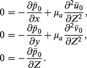
Any realistic lower-dimensional model for the flow should involve effects from both the viscosity and the pressure. We see from (44)-(46) that the limit problem will only satisfy this if m = 2. Indeed, passing to the limit in (44)-(46) with m = 2 yields

$$0=-\frac{\partial {\overline{p}}_0}{\partial x}+\underset{\epsilon \to 0}{\lim }\frac{\partial }{\partial Z}\left({\mu }_{a}r(\beta {\epsilon }^{k-2}{\overline{p}}_0)\frac{\partial {\overline{u}}_0}{\partial Z}\right),$$

(50)

$$0=-\frac{\partial {\overline{p}}_0}{\partial y}+\underset{\epsilon \to 0}{\lim }\frac{\partial }{\partial Z}\left({\mu }_{a}r(\beta {\epsilon }^{k-2}{\overline{p}}_0)\frac{\partial {\overline{v}}_0}{\partial Z}\right),$$

(51)

$$0=\frac{\partial {\overline{p}}_0}{\partial Z}.$$

(52)

We can now distinguish two different cases. If k > 2, then we obtain

$$\begin{array}{l}0=-\frac{\partial {\overline{p}}_0}{\partial x}+{\mu }_a\frac{{\partial }^2{\overline{u}}_0}{\partial Z^2},\\ 0=-\frac{\partial {\overline{p}}_0}{\partial y}+{\mu }_a\frac{{\partial }^2{\overline{v}}_0}{\partial Z^2},\\ 0=-\frac{\partial {\overline{p}}_0}{\partial Z}.\end{array}$$

This system corresponds to a fluid with constant viscosity μ_a and the Reynolds equation may be derived by the same technique that was used in Section A lower-dimensional equation for the pressure: First a change of variables and thereafter asymptotic analysis as $\mathit{\epsilon }\to \mathbf{0}$ , see also Part A of of this study. The conclusion is thus that if k > 2, then the viscosity-pressure coefficient decreases so fast that all piezo-viscous effects disappear in the limit problem. Let us now consider the case k = 2. Indeed, if k = 2, then the system (50)-(52) becomes

$$0=-\frac{\partial {\overline{p}}_0}{\partial x}+{\mu }_{a}r(\beta {\overline{p}}_0)\frac{{\partial }^2{\overline{u}}_0}{\partial Z^2},$$

(53)

$$0=-\frac{\partial {\overline{p}}_0}{\partial y}+{\mu }_{a}r(\beta {\overline{p}}_0)\frac{{\partial }^2{\overline{v}}_0}{\partial Z^2},$$

(54)

$$0=\frac{\partial {\overline{p}}_0}{\partial Z}.$$

(55)

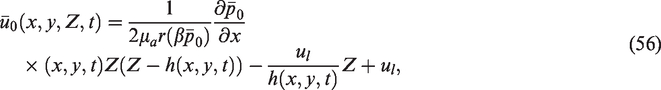
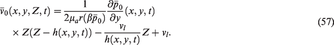
We note that by virtue of (55) it follows that ${\overline{p}}_0$ does not depend on Z. This fact can be used to integrate (53) and (54) twice with respect to Z from 0 to h and by taking the no slip boundary conditions into account we obtain

$$\begin{array}{l}{\overline{u}}_0(x,y,Z,t)=\frac{1}{2{\mu }_{a}r(\beta {\overline{p}}_0)}\frac{\partial {\overline{p}}_0}{\partial x}\\ \times (x,y,t)Z\left(Z-h(x,y,t)\right)-\frac{u_l}{h(x,y,t)}Z+u_l,\end{array}$$

(56)

$$\begin{array}{l}{\overline{v}}_0(x,y,Z,t)=\frac{1}{2{\mu }_{a}r(\beta {\overline{p}}_0)}\frac{\partial {\overline{p}}_0}{\partial y}(x,y,t)\\ \times Z\left(Z-h(x,y,t)\right)-\frac{v_l}{h(x,y,t)}Z+v_l.\end{array}$$

(57)

By inserting these expression for ${\overline{u}}_0$ and ${\overline{v}}_0$ into the associated equation for conservation of mass we can, in a similar way as in Section A lower-dimensional equation for the pressure: First a change of variables and thereafter asymptotic analysis as $\mathit{\epsilon }\to \mathbf{0}$ , derive a Reynolds type of equation for ${\overline{p}}_0$ . Indeed, we obtain

$$\frac{\partial h}{\partial t}=\text{div}\left(\frac{h^3}{12{\mu }_{a}r(\beta {\overline{p}}_0)}\nabla {\overline{p}}_0-\frac{h}{2}V\right),$$

(58)

where $V=u_l\mathbf{i}+v_l\mathbf{j}$ . Expressed in the physical distance between the surfaces $h_{\epsilon }$ , i.e. the film thickness (58) becomes

$$\frac{\partial h_{\epsilon }}{\partial t}=\text{div}\left(\frac{h_{\epsilon }^3}{12{\epsilon }^2{\mu }_{a}r(\beta {\overline{p}}_0)}\nabla {\overline{p}}_0-\frac{h_{\epsilon }}{2}V\right).$$

(59)

Finally, by inserting the approximation $p_{{\epsilon }^{\prime }}={({\epsilon }^{\prime })}^{-2}{\overline{p}}_{{\epsilon }^{\prime }}\approx {({\epsilon }^{\prime })}^{-2}{\overline{p}}_0$ into (59) and making use of the fact that $\alpha =\beta {(\epsilon \prime )}^2$ , we deduce the following lower-dimensional model for the pressure $p_{\epsilon \prime }$ :

$$\frac{\partial h_{\epsilon \prime }}{\partial t}=\text{div}\left(\frac{h_{\epsilon \prime }^3}{12\mu (p_{\epsilon \prime })}\nabla p_{\epsilon \prime }-\frac{h_{\epsilon \prime }}{2}V\right),$$

(60)

which is the piezo-viscous Reynolds equation (2).

For computational purposes it is interesting to note that the nonlinear equation (58) can be linearised carrying out a change of variables. Indeed, let $f({\overline{p}}_0)=1/\left({\mu }_{a}r(\beta {\overline{p}}_0)\right)$ and let F be a function such that $F^{\prime }=f$ . The function f is a strictly positive decreasing function, which implies that F is strictly increasing and hence bijective. We define the new variable

$$\psi (\mathbf{x})=F({\overline{p}}_0(\mathbf{x})),$$

(61)

where $\mathbf{x}=(x,y)$ , and observe that

$$\nabla \psi =F^{\prime }({\overline{p}}_0)\nabla {\overline{p}}_0=f({\overline{p}}_0)\nabla {\overline{p}}_0=\frac{1}{{\mu }_{a}r(\beta {\overline{p}}_0)}\nabla {\overline{p}}_0.$$

(62)

By using the relation (62) we can now express (58) in the new variable as

$$\frac{\partial h}{\partial t}=\text{div}\left(\frac{h^3}{12}\nabla \psi -\frac{h}{2}V\right),$$

(63)

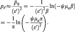
and we see that we now have a linear equation which can be solved easily. When (63) has been solved, then we can find the pressure ${\overline{p}}_0$ by using the relation ${\overline{p}}_0=F^{\text{-}1}(\psi )$ . For instance, if the fluid obey the Barus constitutive law, i.e. $r(s)=e^s$ , then we obtain that

$$\begin{array}{l}{p}_{\epsilon \prime }\approx \frac{{\overline{p}}_0}{{({\epsilon }^{\prime })}^2}=-\frac{1}{{({\epsilon }^{\prime })}^2\beta }\ln (\text{-}\psi {\mu }_a\beta )\\ =-\frac{1}{\alpha }\ln \left(\text{-}\frac{\psi {\mu }_a\alpha }{{({\epsilon }^{\prime })}^2}\right).\end{array}$$

Remark.

In this section we first passed to the limit in the generalised Navier-Stokes equation to obtain a lower-dimensional model for the pressure (the piezo-viscous Reynolds equation). Then we made a change of variables to get a linear lower-dimensional equation which can be used for computing the pressure. In Section A lower-dimensional equation for the pressure: First a change of variables and thereafter asymptotic analysis as $\mathit{\epsilon }\to \mathbf{0}$ , we proceeded the other way around, i.e. we started by doing a change of variables in the generalised Navier-Stokes equation which led to a linear lower-dimensional model when we passed to the limit in the transformed generalised Navier-Stokes equation.

The Reynolds equation: First $\mathit{\alpha }\to \mathbf{0}$ and then $\mathit{\epsilon }\to \mathbf{0}$

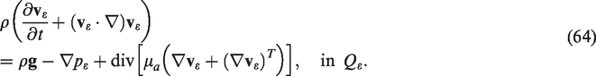
We have so far considered the asymptotic behavior of the solution to the generalised Navier-Stokes equation when the parameters α and ε go to zero simultaneously. In this section, we will consider what happens if we first let α go to zero while ε is fixed and thereafter letting ε go to zero. We will show that in the first step, $\alpha \to 0$ , we obtain the Navier-Stokes equation with constant viscosity. In the second step, $\epsilon \to 0$ , we obtain a limit problem from which the Reynolds equation can be deduced. This is expected, since the Reynolds equation is derived under the assumptions that the fluid is incompressible and that the viscosity is constant, see literature ¹ or Part A of this study. In the existing literature, it is often assumed that the effect of inertia and the body force may be neglected in the derivation of the Reynolds equation. However, as we showed in Part A and as we will see below, this should not be assumed in the derivation since, for incompressible fluids with constant viscosity, it is a consequence of the fluid film being very thin. To this end, we will consider the class of piezo-viscous fluids which may be modeled by the viscosity-pressure relation (42). If we let $\alpha \to 0$ in the equation (3), then we obtain the incompressible Navier-Stokes equation with the constant viscosity μ_a, i.e.

$$\begin{array}{l}\rho \left(\frac{\partial {\mathbf{v}}_{\epsilon }}{\partial t}+\left({\mathbf{v}}_{\epsilon }·\nabla \right){\mathbf{v}}_{\epsilon }\right)\\ =\rho \mathbf{g}-\nabla p_{\epsilon }+\text{div}\left[{\mu }_a\left(\nabla {\mathbf{v}}_{\epsilon }+{(\nabla {\mathbf{v}}_{\epsilon })}^T\right)\right],\text{in} Q_{\epsilon }.\end{array}$$

(64)

We will now study the asymptotic behavior of (64) as the film thickness goes to zero, i.e. as $\epsilon \to 0$ . First we note that since the viscosity is constant, it is possible to use the equation for conservation of mass (4) to rewrite the Navier-Stokes equation (64) as

$$\rho \left(\frac{\partial {\mathbf{v}}_{\mathbf{\epsilon }}}{\partial t}+\left({\mathbf{v}}_{\mathbf{\epsilon }}·\nabla \right){\mathbf{v}}_{\mathbf{\epsilon }}\right)=\rho \mathbf{g}-\nabla p_{\epsilon }+{\mu }_a\Delta {\mathbf{v}}_{\mathbf{\epsilon }}.$$

(65)

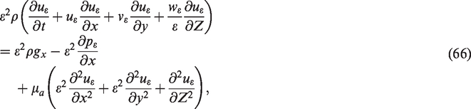
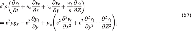
As before, we introduce the fast variable $Z=z/\epsilon ,0<Z<h(x,y,t)$ in order to get a fixed domain. The equation (65) expressed in the fast variable becomes in component form

$$\begin{array}{l}{\epsilon }^2\rho \left(\frac{\partial u_{\epsilon }}{\partial t}+u_{\epsilon }\frac{\partial u_{\epsilon }}{\partial x}+v_{\epsilon }\frac{\partial u_{\epsilon }}{\partial y}+\frac{w_{\epsilon }}{\epsilon }\frac{\partial u_{\epsilon }}{\partial Z}\right)\\ ={\epsilon }^2\rho g_x-{\epsilon }^2\frac{\partial p_{\epsilon }}{\partial x}\\ +{\mu }_a\left({\epsilon }^2\frac{{\partial }^2{u}_{\epsilon }}{\partial x^2}+{\epsilon }^2\frac{{\partial }^2{u}_{\epsilon }}{\partial y^2}+\frac{{\partial }^2{u}_{\epsilon }}{\partial Z^2}\right),\end{array}$$

(66)

$$\begin{array}{l}{\epsilon }^2\rho \left(\frac{\partial v_{\epsilon }}{\partial t}+u_{\epsilon }\frac{\partial v_{\epsilon }}{\partial x}+v_{\epsilon }\frac{\partial v_{\epsilon }}{\partial y}+\frac{w_{\epsilon }}{\epsilon }\frac{\partial v_{\epsilon }}{\partial Z}\right)\\ ={\epsilon }^2\rho g_y-{\epsilon }^2\frac{\partial p_{\epsilon }}{\partial y}+{\mu }_a\left({\epsilon }^2\frac{{\partial }^2{v}_{\epsilon }}{\partial x^2}+{\epsilon }^2\frac{{\partial }^2{v}_{\epsilon }}{\partial y^2}+\frac{{\partial }^2{v}_{\epsilon }}{\partial Z^2}\right),\end{array}$$

(67)

$$\begin{array}{l}{\epsilon }^3\rho \left(\frac{\partial w_{\epsilon }}{\partial t}+u_{\epsilon }\frac{\partial w_{\epsilon }}{\partial x}+v_{\epsilon }\frac{\partial w_{\epsilon }}{\partial y}+\frac{w_{\epsilon }}{\epsilon }\frac{\partial w_{\epsilon }}{\partial Z}\right)\\ ={\epsilon }^3\rho g_z-{\epsilon }^2\frac{\partial p_{\epsilon }}{\partial Z}+{\mu }_a\left({\epsilon }^3\frac{{\partial }^2{w}_{\epsilon }}{\partial x^2}+{\epsilon }^3\frac{{\partial }^2{w}_{\epsilon }}{\partial y^2}+\epsilon \frac{{\partial }^2{w}_{\epsilon }}{\partial Z^2}\right),\end{array}$$

(68)

and the scaled equation for conservation of mass (4) becomes

$$\epsilon \frac{\partial u_{\epsilon }}{\partial x}+\epsilon \frac{\partial v_{\epsilon }}{\partial y}+\frac{\partial w_{\epsilon }}{\partial Z}=0.$$

(69)

With the same motivation as in Section A lower-dimensional equation for the pressure: First a change of variables and thereafter asymptotic analysis as $\mathit{\epsilon }\to \mathbf{0}$ we assume that $u_{\epsilon },v_{\epsilon }$ , and $w_{\epsilon }$ can be written as power series of ε. That is

$$\begin{array}{l}{u}_{\epsilon }(x,y,Z,t)=u_0(x,y,Z,t)+\epsilon u_1(x,y,Z,t)\\ +{\epsilon }^2{u}_2(x,y,Z,t)+\cdots ,\\ v_{\epsilon }(x,y,Z)=v_0(x,y,Z,t)+\epsilon v_1(x,y,Z,t)\\ +{\epsilon }^2{v}_2(x,y,Z,t)+\cdots ,\\ w_{\epsilon }(x,y,Z,t)=w_0(x,y,Z,t)+\epsilon w_1(x,y,Z,t)\\ +{\epsilon }^2{w}_2(x,y,Z,t)+\cdots \end{array}$$

We saw in Subsection Expansion of the velocity field and consequences of the incompressibility condition that the scaled equation for conservation of mass together with the no slip boundary condition on the lower surface imply that $w_0=0.$ Moreover, the no slip boundary condition on the upper surface implies that at the upper surface

$$w_{\epsilon }=\epsilon w_1+{\epsilon }^2{w}_2+\cdots =\frac{\partial h_{\epsilon }}{\partial t}=\epsilon \frac{\partial h}{\partial t},$$

i.e. $w_1=w_1(x,y,h(x,y,t),t)=(\partial h/\partial t)(x,y,t)$ . For most realistic applications in lubrication theory there is a pressure build up in the fluid film because of the relative motion of the surfaces and that the surfaces are not parallel. To keep the influence of the pressure as a dominating effect and not only take plane Couette flow into account we see from (66)-(67) that the dominating term in an expansion of $p_{\epsilon }$ must be of order ${\epsilon }^{-2}.$ Hence, we assume that $p_{\epsilon }$ has an expansion of the form

$$p_{\epsilon }(x,y,Z,t)=\frac{1}{{\epsilon }^2}{\displaystyle \sum _{n=0}^{\infty }{\epsilon }^n}{p}_n(x,y,Z,t).$$

Inserting the expansions of ${\mathbf{v}}_{\epsilon }$ and $p_{\epsilon }$ into (66)-(67) and passing to the limit as $\epsilon \to 0$ yields

$$-\frac{\partial p_0}{\partial x}+{\mu }_a\frac{{\partial }^2{u}_0}{\partial Z^2}=0,$$

(70)

$$-\frac{\partial p_0}{\partial y}+{\mu }_a\frac{{\partial }^2{v}_0}{\partial Z^2}=0,$$

(71)

$$\frac{\partial p_0}{\partial Z}=0.$$

(72)

From (72) we see that p₀ does not depend on z, i.e. $p_0=p_0(x,y,t)$ . This implies that the first two equations in (71) may be integrated with respect to Z. An analysis similar to that in Section A lower-dimensional equation for the pressure: First a change of variables and thereafter asymptotic analysis as $\mathit{\epsilon }\to \mathbf{0}$ leads to the Reynolds type equation

$$\text{div}\left(\frac{h^3}{12{\mu }_a}\nabla p_0-\frac{h}{2}V\right)=\frac{\partial h}{\partial t},$$

(73)

where $V=u_l\mathbf{i}+v_l\mathbf{j}$ . The equation (73) expressed in the physical distance between the surfaces, i.e. $h_{\epsilon }=\epsilon h$ , becomes

$$\text{div}\left(\frac{h_{\epsilon }^3}{{\epsilon }^{2}12\mu }\nabla p_0-\frac{h_{\epsilon }}{2}V\right)=\frac{\partial h_{\epsilon }}{\partial t}.$$

(74)

For small values of ε we have that $p_{\epsilon }\approx {\epsilon }^{-2}{p}_0$ . This together with (74) gives that the classical Reynolds equation yields a good approximation of the physical pressure $p_{\epsilon }$ , i.e.

$$\text{div}\left(\frac{h_{\epsilon }^3}{12\mu }\nabla p_{\epsilon }-\frac{h_{\epsilon }}{2}V\right)=\frac{\partial h_{\epsilon }}{\partial t}.$$

(75)

Remark.

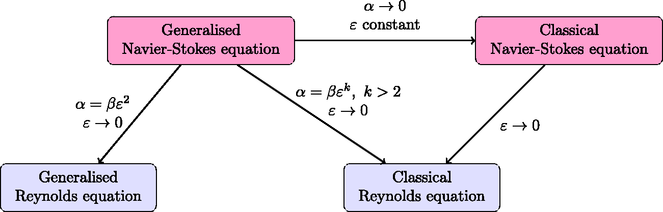
If we first let $\alpha \to 0$ and thereafter let $\epsilon \to 0$ , then we obtain the Reynolds equation (75). We saw in Section A lower-dimensional equation for the pressure: First asymptotic analysis as $\mathit{\epsilon }\to \mathbf{0}$ and thereafter a change of variables that the Reynolds equation is also obtained if we let α and ε go to zero simultaneously under the condition that α is related to ε as $\alpha =\beta {\epsilon }^k,k>2$ , see also Figure 4.

Load carrying capacity and friction force

Two important quantities in the mathematical modeling of lubrication are the friction force and the load carrying capacity. The friction force gives information about the force that has to be applied to keep the surfaces in relative motion and the load carrying capacity is the load carried by the surfaces. In this section, we, will show how our results can be used to find approximations for these fundamental quantities. We will present the ideas by referring to the asymptotic analysis that was carried out in Section A lower-dimensional equation for the pressure: First a change of variables and thereafter asymptotic analysis as $\mathit{\epsilon }\to \mathbf{0}$ .

In Part A we showed that it is only within the context of implicit constitutive relations^3,9,10 that one can rationally obtain a model, wherein the viscosity depends on the mechanical pressure in an incompressible fluid, thereby, giving a proper basis for a constitutive relation of the form

$${\mathit{\sigma }}^{\epsilon }=-p_{\epsilon }I+\mu (p_{\epsilon })\left(\nabla {\mathbf{v}}_{\epsilon }+{(\nabla {\mathbf{v}}_{\epsilon })}^T\right),$$

where μ belongs to the class (42) of viscosity-pressure relations. In particular, we have that

$${\sigma }_{zx}^{\epsilon }=\mu (p_{\epsilon })\left(\frac{\partial w_{\epsilon }}{\partial x}+\frac{\partial u_{\epsilon }}{\partial z}\right)=\mu (p_{\epsilon })\left(\frac{\partial w_{\epsilon }}{\partial x}+\frac{1}{\epsilon }\frac{\partial u_{\epsilon }}{\partial Z}\right),$$

(76)

$${\sigma }_{zy}^{\epsilon }=\mu (p_{\epsilon })\left(\frac{\partial w_{\epsilon }}{\partial y}+\frac{\partial v_{\epsilon }}{\partial z}\right)=\mu (p_{\epsilon })\left(\frac{\partial w_{\epsilon }}{\partial y}+\frac{1}{\epsilon }\frac{\partial u_{\epsilon }}{\partial Z}\right),$$

(77)

$${\sigma }_{zz}^{\epsilon }=-p_{\epsilon }+2\mu (p_{\epsilon })\frac{\partial w_{\epsilon }}{\partial z}=-p_{\epsilon }+\frac{2\mu (p_{\epsilon })}{\epsilon }\frac{\partial w_{\epsilon }}{\partial Z}.$$

(78)

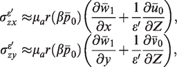
Let us now assume that we want to compute the tangential stresses when $\epsilon =\epsilon \prime$ , i.e. ${\sigma }_{zx}^{{\epsilon }^{\prime }}$ and ${\sigma }_{zy}^{{\epsilon }^{\prime }}$ . We recall the analysis in Section A lower-dimensional equation for the pressure: First asymptotic analysis as $\mathit{\epsilon }\to \mathbf{0}$ and thereafter a change of variables, which showed us that

$$\begin{array}{l}\frac{\partial u_{{\epsilon }^{\prime }}}{\partial Z}=\frac{\partial {\overline{u}}_{{\epsilon }^{\prime }}}{\partial Z}\approx \frac{\partial {\overline{u}}_0}{\partial Z},\frac{\partial v_{{\epsilon }^{\prime }}}{\partial Z}=\frac{\partial {\overline{v}}_{{\epsilon }^{\prime }}}{\partial Z}\approx \frac{\partial {\overline{v}}_0}{\partial Z},\\ \frac{\partial w_{{\epsilon }^{\prime }}}{\partial Z}=\frac{\partial {\overline{w}}_{{\epsilon }^{\prime }}}{\partial Z}\approx \epsilon \prime \frac{\partial {\overline{w}}_1}{\partial Z},\end{array}$$

(79)

$$\begin{array}{l}\mu (p_{{\epsilon }^{\prime }})={\mu }_{a}r(\alpha p_{{\epsilon }^{\prime }})={\mu }_{a}r(\beta \epsilon {\prime }^2{p}_{{\epsilon }^{\prime }})\\ ={\mu }_{a}r(\beta {\overline{p}}_{{\epsilon }^{\prime }})\approx {\mu }_{a}r(\beta {\overline{p}}_0).\end{array}$$

(80)

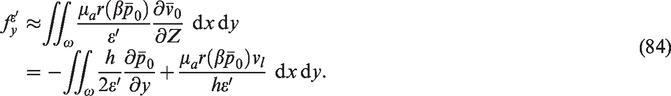
By inserting the approximations (79) and (80) into (76) and (77) we obtain the following approximations for the tangential stresses:

$$\begin{array}{l}{\sigma }_{zx}^{{\epsilon }^{\prime }}\approx {\mu }_{a}r(\beta {\overline{p}}_0)\left(\frac{\partial {\overline{w}}_1}{\partial x}+\frac{1}{{\epsilon }^{\prime }}\frac{\partial {\overline{u}}_0}{\partial Z}\right),\\ {\sigma }_{zy}^{{\epsilon }^{\prime }}\approx {\mu }_{a}r(\beta {\overline{p}}_0)\left(\frac{\partial {\overline{w}}_1}{\partial y}+\frac{1}{{\epsilon }^{\prime }}\frac{\partial {\overline{v}}_0}{\partial Z}\right),\end{array}$$

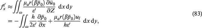
Hence, since ${\overline{w}}_1(x,y,0,t)=0$ , the friction ${\mathbf{F}}_{{\epsilon }^{\prime }}=(f_x^{{\epsilon }^{\prime }},f_y^{{\epsilon }^{\prime }})$ at the lower surface is

$$f_x^{{\epsilon }^{\prime }}={\displaystyle {\iint }_{\omega }{\sigma }_{zx}^{{\epsilon }^{\prime }}}\text{d}x\text{d}y\approx {\displaystyle {\iint }_{\omega }\frac{{\mu }_{a}r(\beta {\overline{p}}_0)}{{\epsilon }^{\prime }}}\frac{\partial {\overline{u}}_0}{\partial Z}\text{d}x\text{d}y,$$

(81)

$$f_y^{{\epsilon }^{\prime }}={\displaystyle {\iint }_{\omega }{\sigma }_{zy}^{{\epsilon }^{\prime }}}\text{d}x\text{d}y={\displaystyle {\iint }_{\omega }\frac{{\mu }_{a}r(\beta {\overline{p}}_0)}{{\epsilon }^{\prime }}}\frac{\partial {\overline{v}}_0}{\partial Z}\text{d}x\text{d}y,$$

(82)

where ω is the lower surface (Z = 0), see Section Notation, a change of variables and problem formulation. We can now use (56) and (57) to express ${\overline{u}}_0$ and ${\overline{v}}_0$ in ${\overline{p}}_0$ , which implies that (81) and (82) can be written as

$$\begin{array}{l}{f}_x^{{\epsilon }^{\prime }}\approx {\displaystyle {\iint }_{\omega }\frac{{\mu }_{a}r(\beta {\overline{p}}_0)}{{\epsilon }^{\prime }}}\frac{\partial {\overline{u}}_0}{\partial Z}\text{d}x\text{d}y\\ =-{\displaystyle {\iint }_{\omega }\frac{h}{2\epsilon \prime }}\frac{\partial {\overline{p}}_0}{\partial x}+\frac{{\mu }_{a}r(\beta {\overline{p}}_0)u_l}{h\epsilon \prime }\text{d}x\text{d}y,\end{array}$$

(83)

$$\begin{array}{l}{f}_y^{{\epsilon }^{\prime }}\approx {\displaystyle {\iint }_{\omega }\frac{{\mu }_{a}r(\beta {\overline{p}}_0)}{{\epsilon }^{\prime }}}\frac{\partial {\overline{v}}_0}{\partial Z}\text{d}x\text{d}y\\ =-{\displaystyle {\iint }_{\omega }\frac{h}{2\epsilon \prime }}\frac{\partial {\overline{p}}_0}{\partial y}+\frac{{\mu }_{a}r(\beta {\overline{p}}_0)v_l}{h\epsilon \prime }\text{d}x\text{d}y.\end{array}$$

(84)

Expressed in the physical distance $h_{{\epsilon }^{\prime }}$ and the pressure $p_{{\epsilon }^{\prime }}$ this becomes

$$f_x^{{\epsilon }^{\prime }}\approx -{\displaystyle {\iint }_{\omega }\frac{h_{{\epsilon }^{\prime }}}{2}}\frac{\partial p_{{\epsilon }^{\prime }}}{\partial x}+\frac{\mu (p_{{\epsilon }^{\prime }})u_l}{h_{{\epsilon }^{\prime }}}\text{d}x\text{d}y,$$

(85)

$$f_y^{{\epsilon }^{\prime }}\approx -{\displaystyle {\iint }_{\omega }\frac{h_{{\epsilon }^{\prime }}}{2}}\frac{\partial p_{{\epsilon }^{\prime }}}{\partial y}+\frac{\mu (p_{{\epsilon }^{\prime }})u_l}{h_{{\epsilon }^{\prime }}}\text{d}x\text{d}y.$$

(86)

To compute ${\mathbf{F}}_{{\epsilon }^{\prime }}$ via (83) and (84) we must know ${\overline{p}}_0$ . The equation (58) for ${\overline{p}}_0$ is nonlinear and from a computational point of view it is often beneficial to linearize the equation by using the change of variables (61).

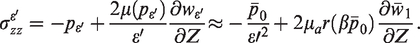
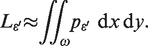
Let us now discuss how to obtain an approximation of the load carrying capacity $L_{\epsilon }$ . By combining (79) and (78) we obtain that for $\epsilon =\epsilon \prime$ the normal stress

$${\sigma }_{zz}^{{\epsilon }^{\prime }}=-p_{{\epsilon }^{\prime }}+\frac{2\mu (p_{{\epsilon }^{\prime }})}{{\epsilon }^{\prime }}\frac{\partial w_{{\epsilon }^{\prime }}}{\partial Z}\approx -\frac{{\overline{p}}_0}{\epsilon {\prime }^2}+2{\mu }_{a}r(\beta {\overline{p}}_0)\frac{\partial {\overline{w}}_1}{\partial Z}.$$

However, at the lower surface, the last term is zero. Indeed, by virtue of the no slip boundary conditions it follows that $\partial {\overline{u}}_0/\partial x=\partial {\overline{v}}_0/\partial y=0$ on ω, which together with the associated equation for conservation of mass implies that $\partial w_1/\partial Z=0$ on ω. We can now find an approximate expression for the load carrying capacity

$$L_{{\epsilon }^{\prime }}:=-{\displaystyle {\iint }_{\omega }{\sigma }_{zz}^{{\epsilon }^{\prime }}}\text{d}x\text{d}y\approx {\displaystyle {\iint }_{\omega }\frac{{\overline{p}}_0}{\epsilon {\prime }^2}}\text{d}x\text{d}y,$$

(87)

or expressed in terms of the physical pressure

$$L_{{\epsilon }^{\prime }}\approx {\displaystyle {\iint }_{\omega }{p}_{{\epsilon }^{\prime }}}\text{d}x\text{d}y.$$

Numerical examples illustrating the convergence

To be able to conduct a meaningful case study of a realistic EHL problem, one would have to (at least) include both cavitation and elastic deformation, which we are not yet able to include on the same rigorous level as we now are able to include that the viscosity depends on the pressure. Mixing our well-motivated mathematical results with available results for cavitation and elastic deformation, that are not at all as well-motivated, would therefore be misleading for the reader. With the numerical examples presented here we will, therefore, merely illustrate the efficiency of our theoretical results in accounting for a pressure dependency in the viscosity. This will be done in two examples that compare analytical pressure solutions, pressure solutions obtained by solving the lower-dimensional models which have been derived and pressure solutions obtained by solving the generalised Navier-Stokes together with the equation for the conservation of mass.

To present the numerical result, one must chose a viscosity-pressure relation and describe the distance between the surfaces. We chose the Barus constitutive law (5) and a tilted linear slider bearing. To illustrate our theoretical results it suffices to consider an infinitely wide bearing. Hence, $\omega =\left\{x\in ℝ:0<x<L_x\right\}$ , and the film thickness may be mathematically modelled as

$$h(x)=h_{\max }-\frac{h_{\max }-h_{\min }}{L_x}x.$$

(88)

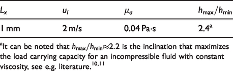
Table 1 lists input data common for both examples.

Table 1.

Input parameters common to both examples.

Lx	ul	μa	$h_{\max }/h_{\min }$
1 mm	2 m/s	0.04 Pa $·$ s	2.4a

a

It can be noted that $h_{\max }/h_{\min }\approx 2.2$ is the inclination that maximizes the load carrying capacity for an incompressible fluid with constant viscosity, see e.g. literature.^10,11

The pressure solutions to the generalised Navier-Stokes equation obtained with the Laminar Flow Interface in COMSOL multiphysics, ¹² were performed on a regular grid with 200 elements in the x-direction and 20 in the z-direction. Quadratic shape functions were used for the velocity and linear for the pressure, which may be employed in COMSOL multiphysics by selecting the $\text{P}2+\text{P}1$ option for the discretisation. The pressure solutions of the lower-dimensional model was implemented as a Coefficient Form Boundary PDE, with the lower boundary ω (of the fluid domain $Q_{\epsilon }$ ) defining the solution domain. It was discretised using quadradic lagrange elements and the mesh with 200 elements for ω, inherited from the Laminar Flow Interface.

Example 1

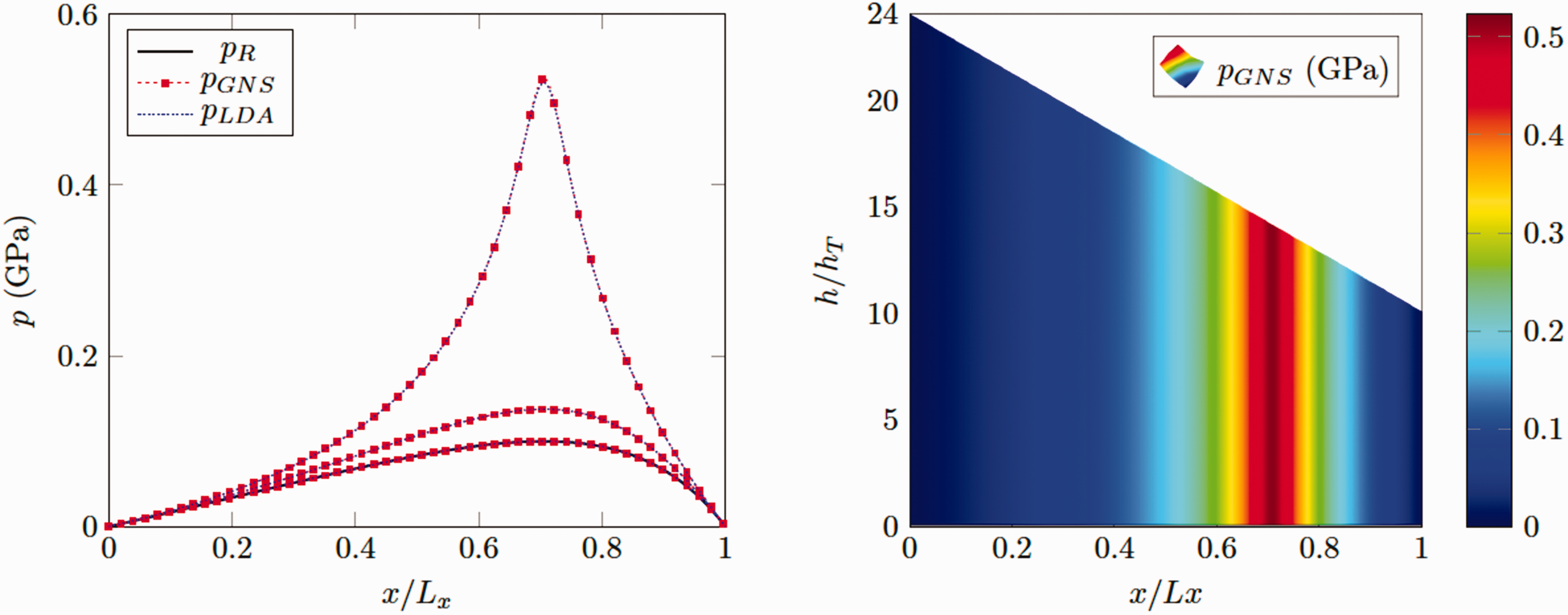
In the left part of Figure 2, pressure solutions for the four α-values given in Table 2 are depicted. For the three nonzero values of α, the pressure distribution p_LDA (continuous black line) obtained by the lower-dimensional algorithm, presented in Section Computing the pressure via inverse transformation, have been compared to the pressure solution p_GNS (dashed red line) to the generalised Navier-Stokes equation at z = 0. The special case α = 0, i.e. when the viscosity μ_a is constant, renders the classical incompressible solution to the Reynolds equation (1) and this solution, denoted p_R is also depicted (blue dashed line) in Figure 2. Firstly, it can be observed that as α decreases, the pressure distribution approaches the one corresponding to the case with constant viscosity, which agrees with our analysis. Secondly, it can be seen that each pressure distribution obtained by the lower-dimensional algorithm (p_LDA) (for this particular example problem) is in principle identical with the one given by the generalised Navier-Stokes equation at z = 0 (p_GNS). Moreover, for α = 0 all three pressure solutions are visually indistinguishable. In Section A lower-dimensional equation for the pressure: First a change of variables and thereafter asymptotic analysis as $\mathit{\epsilon }\to \mathbf{0}$ , we saw that q₀ does not depend on Z, see (30), which implies that the pressure does not vary across the film. This is illustrated in the Figure 2 (right), where p_GNS is depicted for α = 10 GPa^{– 1} .

Figure 2.

Left: Comparison of pressure solutions p_LDA obtained by the lower-dimensional algorithm (dashed blue line) with pressure solutions p_GNS to the generalised Navier-Stokes equation, obtained using the Laminar Flow Interface in COMSOL multiphysics ¹² (dotted red line). The pressure solution p_R to Reynolds’ equation (1) (continuous black line) can also be seen in the figure. Right: Illustration of that the pressure is constant across the fluid film.

Table 2.

The values of α used in Example 2.

α (GPa– 1)

10

5

0.1

0

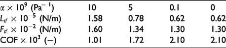
We computed the load carrying capacity $L_{{\epsilon }^{\prime }}$ for the nonzero values of α by using (87). The results are presented in Table 3. We also computed the friction force $F_{{\epsilon }^{\prime }}$ using (83) and the numerical results are collected in Table 3. The numerical values of the coefficient of friction $\text{COF}$ ( $F_{{\epsilon }^{\prime }}/L_{{\epsilon }^{\prime }}$ ) are also included in Table 3.

Table 3

Load carrying capacity $L_{\epsilon }$ , friction force $F_{\epsilon }$ and Coefficient of Friction (COF) for different values of α.

$\alpha \times {10}^9$ (Pa– 1)	10	5	0.1	0
$L_{\epsilon \prime }\times {10}^{-5}$ (N/m)	1.58	0.78	0.62	0.62
$F_{\epsilon \prime }\times {10}^{-2}$ (N/m)	1.60	1.34	1.30	1.30
$\text{COF}\times {10}^3$ (−)	1.01	1.72	2.10	2.10

Example 2

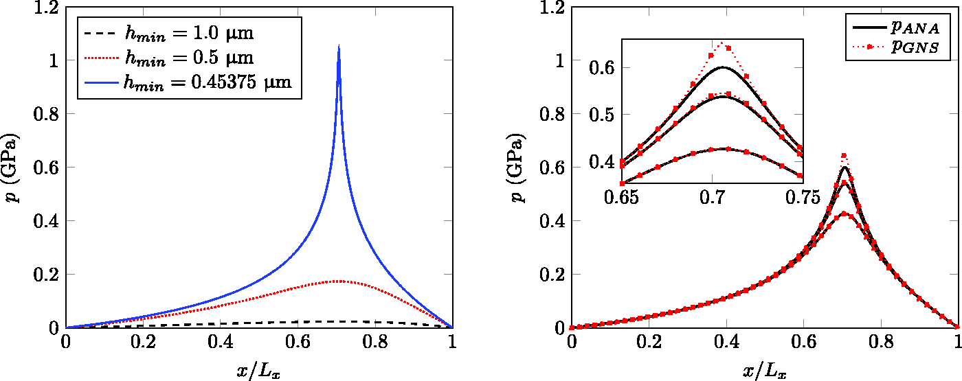
For the set of input parameters listed in Table 1 and α = 10 GPa^{– 1} the analytical pressure solution, derived in The Appendix, approaches its maximum value $p_{\max }\approx 1.03$ GPa as $h_{\min }\to 0.45374$ µm. Three pressure distributions corresponding to the parameters in Table 1 and h_min = 1, 0.5 and 0.45375 µm, are depicted in the left side of Fig. 3.

Figure 3.

Left: The analytical pressure solution corresponding to the input parameters given in Table 1 and α = 10 GPa^{– 1} for h_min = 1, 0.5 and 0.45375 µm. Right: The analytical solution (p_ANA) (continuous black line) and the numerical solution to the generalised Navier-Stokes equation (p_GNS) (dashed red line), corresponding to the input parameters given in Table 1 and h_min = 0.45375 µm for $\alpha =9.8500$ , 9.95281 and 9.97516 GPa^{– 1} (right). The insert shows a magnification of the maximum pressure region.

The right side of Fig. 3 depicts the analytical solution and the numerical solution of the generalised Navier-Stokes equation (3), solved together with the equation for the conservation of mass (4), for three different values of $\alpha =9.85000$ , 9.95281 and 9.97516 GPa^{– 1} . It can be seen that the solutions are more or less identical for the smallest of the α-values, but that a discrepancy develops as α increase. Indeed, the solutions to the lower-dimensional model (p_ANA) and the generalised Navier-Stokes equations (p_GNS) will differ in the limit, if the film thickness and α are not coupled, as explained by the asymptotic analysis in Section A lower-dimensional equation for the pressure: First a change of variables and thereafter asymptotic analysis as $\mathit{\epsilon }\to \mathbf{0}$ .

We remark that the reason for varying α instead of the film thickness, is due to that the film thickness is related to the geometry. The solution for $\alpha =9.97516$ GPa^{– 1} is the last converged solution in the range $[9.85000,9.99900]$ GPa^{– 1} of 101 uniformly separated values. These were obtained with the Auxiliary Sweep Study Extension available in COMSOL multiphysics. An attempt To get closer to an α-value of 10 GPa^{– 1} a mesh densification around $x/L_x=12/17\approx 0.705$ (where the maximum pressure occurs in this case) was also implemented. It did, however, not facilitate the auxiliary sweep to come any closer to $\alpha =9.99900$ GPa^{– 1} , than 9.97516 GPa^{– 1} , which was already obtained with the regular mesh consisting of 200 × 20 elements. This supports that the discrepancies betwen the solutions are not dominated by numerical errors, but comes from that the models are different.

Concluding remarks

In lubrication theory it is common to assume, often in a quite heuristic way, that it is possible to just replace the constant viscosity in the Reynolds equation with a viscosity-pressure relationship. In particular, this is the case in elastohydrodynamic lubrication and its correctness has been the subject matter of discussion, see e.g. literature. ² In this paper, we have shown that it is correct, if the coefficient α in the viscosity-pressure relation (42) is small, which it is in many realistic applications. We have done this by studying the asymptotic behavior of the generalised Navier-Stokes equation as the film thickness goes to zero, i.e. as $\epsilon \to 0$ , in two different ways. In Section A lower-dimensional equation for the pressure: First a change of variables and thereafter asymptotic analysis as $\mathit{\epsilon }\to \mathbf{0}$ , we made a change of variables before the asymptotic analysis, whereas we in Section A lower-dimensional equation for the pressure: First asymptotic analysis as $\mathit{\epsilon }\to \mathbf{0}$ and thereafter a change of variables first carried out the asymptotic analysis and thereafter made a change of variables in the limit problem.

In order to get a limit problem which makes sense, it was conluded that α must decrease with ε. We found that a correct scaling is $\alpha =\beta {\epsilon }^k$ , where $\beta >0$ and $k\ge 2$ . In the case k = 2 the effects of the piezo-viscosity is captured as $\epsilon \to 0$ and we obtain the generalised Reynolds equation (2). If k > 2, then α goes towards zero so fast, as $\epsilon \to 0$ , so that the piezo-viscous effect disappears and we obtain the classical Reynolds equation with constant viscosity μ_a. We have also shown that, if we keep ε fixed and let $\alpha \to 0$ in the generalised Navier-Stokes equation, then we get the classical Navier-Stokes equation. Moreover, we have seen that we obtain the classical Reynolds equation by letting $\epsilon \to 0$ in the classical Navier-Stokes equation. The convergence results are illustrated in Figure 4. In connection to this, we have illustrated by means of some numerical examples that the pressure solutions obtained by our lower-dimensional algorithms are in very good agreement with the pressure solutions obtained by solving the generalised Navier-Stokes equation.

Figure 4.

Illustration of the convergence results.