Sage Journals: Discover world-class research

Abstract

This study aimed to develop an effective forecasting model for daily average PM_2.5 concentration using a multilayer perceptron (MLP) neural network. The model was applied to 3 air quality monitoring stations in Mashhad, Iran—Sajjad, Torogh, and Vila—representing different urban land use types. A separate network was trained for each station. The optimal network architecture was determined by tuning the number of neurons in the hidden layer, using input variables such as the previous day’s meteorological parameters (wind speed, temperature, precipitation, solar radiation, and relative humidity), PM_2.5 concentration, and temporal indicators (day of the week and month). Data standardization and early stopping were used to enhance generalization. The model performed best at Sajjad station, with an R² of .79 and MAE of 5.54 µg/m³. Performance at Torogh was acceptable, while Vila showed weaker results. The model detected PM_2.5 exceedance events with a true positive rate of 66% to 74% and a false alarm rate as low as 0.18 at Sajjad. Differences in topography, pollution sources, and microclimate conditions influenced spatial variability in accuracy. These findings suggest that MLP neural networks are effective tools for daily air pollution prediction and can support localized early warning systems.

Plain Language Summary

Air pollution, especially tiny particles known as PM_2.5, poses serious risks to human health. This study evaluated the ability of a machine-learning model to predict next-day PM_2.5 concentrations at three monitoring sites in Mashhad, Iran. A multilayer perceptron (MLP) neural network was trained using previous-day observations of PM_2.5 and meteorological variables (temperature, humidity, wind speed, and precipitation), together with temporal categorical features (day-of-week and month). Model performance was compared across sites with different local conditions. Forecast accuracy was higher at locations with more stable emission patterns and lower at sites affected by complex topography and mixed sources. The results indicate that site-specific, properly preprocessed MLP models can provide useful next-day PM_2.5 forecasts to support local early-warning and exposure-mitigation measures.

Keywords

artificial neural networks air pollution urban monitoring station meteorological data

Introduction

One of the critical factors affecting public health is air quality, which is largely influenced by the concentration of particulate matter. Among these, fine particulate matter with a diameter of less than 2.5 micrometers (PM_2.5) has been widely recognized for its direct association with adverse health effects.^1,2 Elevated levels of PM_2.5 have been linked to changes in lifestyle, reduced life expectancy, and increased mortality rates. Numerous studies have demonstrated a statistically significant correlation between atmospheric PM_2.5 concentrations and negative health outcomes.³ Consequently, various air quality standards for PM_2.5 have been established based on hourly, daily, and annual exposure limits. According to the latest guidelines of the World Health Organization, the recommended annual and 24-hour average limits for PM_2.5 are 5 and 15 µg/m³, respectively.⁴ In Iran, based on the national air quality standard approved in 2016, these thresholds are set at 12 and 35 µg/m³, respectively.⁵

Meteorological factors such as wind speed and direction, temperature, precipitation, and planetary boundary layer height significantly influence the variability of PM_2.5 concentrations in the atmosphere.⁶ Severe air pollution episodes typically occur in regions where geographical features and atmospheric stability inhibit natural ventilation, leading to the accumulation of pollutants like PM_2.5.⁷ These particles, primarily emitted from combustion sources such as urban traffic and industrial activities, remain suspended in the atmosphere for extended periods due to their ultrafine size and can rapidly reach critical concentration levels.⁸ Under such conditions, immediate interventions—such as traffic restrictions, school closures, or the suspension of polluting activities—are often required. Accordingly, both national and international air pollution control regulations mandate the implementation of automated operational procedures to prevent pollutant concentrations from exceeding predefined alert thresholds. Here, automated operational procedures denote pre-programed, rule-based response protocols that are activated automatically by real-time monitoring data or short-term forecasts when predefined conditions are met.^4,5 These protocols implement explicit decision rules (eg, if forecasted daily PM_2.5 reaches or exceeds the action level, then trigger the predefined mitigation measure) and commonly include automated public and institutional alerts (SMS, mobile apps, variable-message signs), traffic-management measures (temporary restrictions, adaptive signal control), notifications to industrial operators to curtail emissions, and rapid deployment of dust-suppression and street-cleaning operations to reduce resuspension of road and construction dust, which contribute to ambient PM concentrations. Automation ensures a rapid, coordinated, and consistent response that reduces delays and human-decision variability.

Mashhad, one of Iran’s major and densely populated metropolitan cities, exhibits both urban and semi-industrial characteristics due to its religious, touristic, and industrial significance. A substantial portion of PM_2.5 emissions in Mashhad originates from mobile sources, including older vehicles, diesel buses, and motorcycles. While household heating in most areas of the city is primarily supplied through natural gas systems, in suburban districts such as Toos, Torogh, and surrounding villages, the use of liquid fuels—such as kerosene and diesel—remains prevalent. This reliance on liquid fuels, particularly during colder months, can lead to localized increases in PM_2.5 concentrations. In addition to anthropogenic sources, natural contributors such as windblown dust from nearby desert regions also play a role in elevating ambient PM_2.5 levels.⁹

Given the health impacts associated with PM_2.5, this pollutant has become a major public concern in the city of Mashhad. Forecasting PM_2.5 concentrations prior to pollution episodes can facilitate more effective interventions to protect public health. A wide range of operational early warning systems—based on statistical and hybrid modeling approaches—have been developed to enable proactive and real-time responses to air pollution events. In this context, predictive models have been increasingly utilized as supportive tools for air quality management in various regions around the world.

Artificial neural networks (ANNs) have been widely applied to forecast the concentrations of various pollutants over different time scales, yielding promising results.^10,11 In air quality prediction studies, methods such as ANNs, multiple linear regression (MLR), and stepwise regression (SWR) are among the most commonly used approaches.¹² Due to the complex and nonlinear relationships between meteorological parameters and pollution levels, ANNs have demonstrated superior performance compared to traditional statistical models.¹³ Since their initial application in modeling atmospheric pollutant concentrations,¹⁴ ANNs have been regarded as a reliable method in this field.

Although forecasting particulate matter concentrations is more complex than modeling gaseous pollutants—due to the intricate processes involved in aerosol formation, transport, and removal¹⁵—neural networks have demonstrated high accuracy owing to their ability to identify and model nonlinear relationships.¹⁶ Feedforward neural networks with error backpropagation (FFNNs) are among the most commonly used neural network architectures for predicting pollutants such as PM_2.5, PM₁₀, O₃, SO₂, and CO, due to their capacity to model complex nonlinear interactions.¹⁷ In one study, several machine learning methods were used to predict PM_2.5 exceedance events, and FFNNs exhibited superior performance.¹⁸ In other studies, various machine learning approaches—including FFNNs, pruned neural networks (PNNs), and lazy learning (LL) techniques—have been applied for PM_2.5 concentration prediction, with FFNNs consistently outperforming the alternatives.¹⁹ Another study analyzed multiple methods for forecasting daily average PM_2.5 concentrations. The results of 2 types of multilayer perceptron (MLP) networks—an important subclass of FFNNs—and a radial basis function (RBF) network were compared with 2 classical models, and the MLP model demonstrated superior predictive performance.²⁰

In the present study, a model was developed to predict daily PM_2.5 concentrations based on air pollution data collected from 3 monitoring stations—Sajjad, Vila, and Torogh—in the city of Mashhad. These stations represent diverse urban conditions: the Sajjad station is located in a densely populated, high-traffic area; the Vila station is situated in a region with moderate population density; and the Torogh station is positioned on the southeastern outskirts of the city, where air quality is influenced by industrial activities and heavy-duty vehicle traffic.

An MLP neural network was employed to predict the daily average PM_2.5 concentrations at the selected monitoring stations. Model inputs included the previous day’s average PM_2.5 concentration as well as the previous day’s meteorological parameters, such as mean wind speed and direction, precipitation, solar radiation, temperature, and relative humidity. Additionally, to account for variations in traffic patterns across different days of the week and throughout the year—due to Mashhad’s religious and touristic nature—variables such as the day of the week (1 -7) and the month of the year (1 -12) were incorporated into the model as input features. The primary objective of this study is to protect at-risk populations by providing accurate and timely information on air quality.

The novelty of this study lies in the development and application of ANN models to predict daily PM_2.5 concentrations in Mashhad, one of Iran’s most polluted metropolitan areas. Unlike previous studies that have mainly focused on descriptive assessments of air quality or conventional statistical approaches, our work integrates meteorological variables with traffic-related temporal factors (day of the week and month of the year) to build robust predictive models tailored to the local conditions of Mashhad. By evaluating the performance of multiple ANN training algorithms and comparing prediction accuracy across different urban monitoring stations with diverse land uses, this study provides new insights into the spatial and temporal variability of PM_2.5 in the city. The outcomes not only advance the methodological framework for air pollution forecasting in developing countries but also offer practical implications for automated early-warning systems and evidence-based air quality management.

Materials and Methods

Design and Training of MLP Neural Networks

In this study, 3 MLP neural networks were developed to predict the daily average concentration of PM_2.5 at 3 air quality monitoring stations in Mashhad: Sajjad, Torogh, and Vila. Each network was independently designed and trained for a specific station—ANN1 for Sajjad, ANN2 for Torogh, and ANN3 for Vila.

The initial dataset comprised several years of hourly pollutant concentrations and meteorological parameters. These data were preprocessed using the Python programing language, with the aid of the pandas library for structured data manipulation and NumPy for numerical computations. During preprocessing, the data were time-indexed by date and aggregated into daily values (24-hour averages) to enable the prediction of next-day PM_2.5 concentrations. In instances where one or more input variables were missing for a given day, the corresponding row was removed from the dataset to avoid errors associated with imputation of missing values. Ultimately, approximately 80% of the daily data for each station remained complete and was deemed suitable for model development.

The general architecture of each network consisted of 3 main layers: an input layer, a hidden layer, and an output layer. The input layer incorporated the modeling variables, including meteorological and air quality parameters. The hidden layer comprised several neurons that computed the weighted sum of the inputs and passed the results through a nonlinear tangent sigmoid activation function. The final output was produced in the output layer by combining the weighted outputs of the hidden layer neurons using a linear activation function.

The use of the tangent sigmoid function in the hidden layer enables the network to capture nonlinear mappings and model complex relationships, while the linear activation function in the output layer ensures the generation of continuous outputs without additional nonlinear transformation. This combination of activation functions provides an efficient modeling framework for predicting PM_2.5 concentrations.²¹

To identify the most appropriate training algorithm for each station, initial neural networks with 10 neurons in the hidden layer were designed and trained using several algorithms. The performance of each algorithm was evaluated on the training, validation, and testing datasets using statistical performance metrics. The algorithm yielding the best overall performance was selected for further modeling.

Once the optimal training algorithm was identified, the process of determining the optimal number of neurons in the hidden layer for each network began. Networks were initially trained with 10 neurons, and the number of neurons was then gradually increased to assess different network configurations. For each configuration, statistical performance indicators were recorded and analyzed for the training, validation, and testing sets. This process continued until the most efficient network structure—based on performance metrics—was identified for each monitoring station.

To prevent overfitting, network structures that exhibited decreased training error but increased validation or testing error were excluded. Network training was performed using the backpropagation algorithm, aiming to minimize the discrepancy between predicted and actual outputs. This process involved a forward pass for signal propagation and a backward pass for updating the connection weights through error backpropagation.

The modeling process was conducted using MATLAB software. The dataset for each station was randomly shuffled and split into training (70%), validation (15%) and test (15%) subsets to mitigate overfitting. The total number of daily data points was 1771 for Sajjad, 1706 for Torogh, and 1641 for Vila; accordingly, the independent test sets comprised 266 (Sajjad), 256 (Torogh), and 246 (Vila) daily samples. The early stopping method was employed to further reduce the risk of overfitting. Additionally, to enhance the stability and reliability of the results, each network was independently trained 3 times.

Study Area

This study was conducted in the metropolitan city of Mashhad, located in northeastern Iran. With a population exceeding 3.5 million, Mashhad is the second most populous city in the country after Tehran. Due to its religious and touristic significance, the city attracts over 20 million domestic and international pilgrims and tourists annually. These characteristics have led to high urban traffic density, increased fossil fuel consumption, and the expansion of commercial and service activities—major sources of PM_2.5 emissions.

Topographically, Mashhad is situated on a plain at an average elevation of approximately 980 m above sea level. It is surrounded by the Hezar-Masjed Mountains to the north (with elevations exceeding 2800 m) and the Binalood Range to the southwest (reaching approximately 3211 m). This complex terrain gives rise to specific climatic phenomena such as mountain-to-plain breezes, nocturnal temperature inversions during cold nights, and convective airflows in warmer seasons. These conditions can contribute to elevated pollutant concentrations or the persistence of pollutants near the surface, particularly during winter when thermal inversion events are more intense.

The average annual temperature in Mashhad is approximately 12.4 °C, and the mean annual precipitation is reported to be around 248.6 mm. The prevailing winds in this region typically blow from the west and northwest, with an average speed of about 3 m/s.²² On average, approximately 86 days per year in Mashhad are classified as having unhealthy air quality for sensitive groups—including children, the elderly, and individuals with respiratory illnesses. This condition is primarily attributed to combustion-related sources such as heavy traffic congestion, domestic heating, industrial activities, and regional climatic factors.²³

In this study, data from 3 air quality monitoring stations were used, each located in areas with distinct environmental characteristics and pollution sources. The Sajjad station was selected to represent urban background pollution associated with PM_2.5. This station is situated in the city center at an elevation of approximately 1000 m above sea level, near Falasteen Square, and within less than 100 m of major roads such as Sajjad and Ahmadabad Boulevards. This area is among the busiest traffic zones in Mashhad and is significantly influenced by emissions from both light and heavy vehicles.

The Torogh station, located in the southeastern part of Mashhad at an elevation of approximately 1020 m above sea level, lies about 15 km from the city center and near the Torogh Industrial Zone. This station reflects the combined impact of pollution from high diesel vehicle traffic, industrial activities, and emissions from heavy-duty transportation sources.

The Vila station is situated in a mixed residential-commercial area with moderate traffic density in the southwestern part of the city, at an elevation of approximately 970 m. It is located about 5 km from the city center and is relatively distant from direct sources of industrial emissions. Therefore, this station is considered representative of areas with lower background pollution levels.

The geographic coordinates of the monitoring stations used in this study are as follows: Vila Station (36.31681°N, 59.48475°E), Sajjad Station (36.31854°N, 59.55464°E), and Torogh Station (36.21007°N, 59.66678°E). Additionally, the meteorological station is located at 36.25452° N, 59.61774°E. These coordinates were used to accurately plot the spatial distribution of the monitoring sites on the topographic map of Mashhad, enabling a clearer understanding of their positions in relation to surrounding emission sources and land use patterns.

Figure 1 presents the topographic map of Mashhad, illustrating the locations of the 3 PM_2.5 monitoring stations (Sajjad, Vila, and Torogh) as well as the meteorological station. To enhance spatial interpretation, the map also indicates major potential sources of PM_2.5 emissions, including 2 large industrial zones on the city’s outskirts, Mashhad International Airport, adjacent desert regions, densely populated residential neighborhoods, and central business districts (CBDs). These features are schematically represented based on their approximate locations relative to the monitoring stations.

Figure 1.

Topographic map of Mashhad showing the locations of PM_2.5 monitoring stations (Sajjad, Torogh, Vila) and the meteorological station, along with major sources of PM_2.5 emissions (industrial zones, airport, desert areas, central business districts, and residential zones).

Data Preparation

Daily datasets for the 3 monitoring stations in Mashhad (Sajjad, Vila, and Torogh) were compiled for 2018 to 2023, including meteorological parameters—air temperature (°C), relative humidity (%), average wind speed (m/s), wind direction (degrees), and precipitation (mm)—and PM_2.5 concentrations. Meteorological data were obtained from the Khorasan Razavi Meteorological Organization, while PM_2.5 data were provided by the Khorasan Razavi Department of Environment.

PM_2.5 concentrations were recorded hourly using online beta attenuation monitors. In this method, an airstream passes over a filter, and the resulting decrease in beta radiation intensity is used to calculate PM_2.5 mass concentration. Although beta attenuation monitors are semi-reference methods,²⁴ data were corrected using adjustment coefficients derived from comparisons with gravimetric reference methods when necessary. Data coverage over the study period was approximately 80% for each station. To maintain analytical integrity, no extrapolation or interpolation was performed to replace missing data.

Annual average PM_2.5 concentrations ranged from 35-38 μg/m³ at Sajjad, 26-32 μg/m³ at Torogh, and 20-28 μg/m³ at Vila, reflecting variations in local emission sources such as traffic, industrial activity, and domestic heating.

To provide an overview of the statistical characteristics of the dataset used in this study, descriptive indicators—including range, mean, and standard deviation—were calculated for the main parameters (PM_2.5 concentration, temperature, humidity, wind speed, and precipitation). The results of this statistical analysis are presented in Table 1. These indicators help identify data variability and offer insights into the distribution of variables over the study period.

Table 1.

Descriptive Statistics of Meteorological Variables and PM_2.5 Concentrations Over the 6-Year Period (2018-2023).

Variable	Range	Mean	Standard deviation
PM_2.5 concentration at Sajjad Station (µg/m³)	112.08	36.54	18.81
PM_2.5 concentration at Torogh Station (µg/m³)	151.23	29.97	26.43
PM_2.5 concentration at Vila Station (µg/m³)	140.00	22.30	23.03
Average precipitation (mm)	49.80	0.56	2.55
Maximum temperature (°C)	52.90	23.35	10.29
Average temperature (°C)	48.70	16.81	9.18
Maximum wind speed (m/s)	18.00	6.99	2.59
Average wind speed (m/s)	9.50	3.04	1.07
Average relative humidity (%)	88.25	49.04	21.68

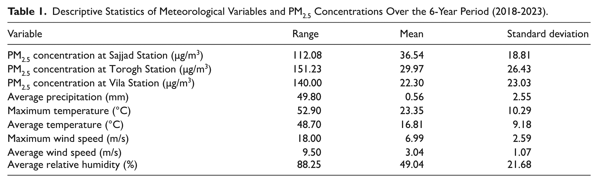
These values indicate considerable variability in both pollutant concentrations and meteorological conditions, which is crucial for understanding the dynamics of PM_2.5 behavior and its interaction with environmental parameters in the urban context of Mashhad.

As shown in Table 1, the variables under investigation exhibit different numerical ranges. For example, PM_2.5 concentrations at the Sajjad station have a range of 112.08 µg/m³, while the average wind speed varies over a range of 9.50 m/s. These wide disparities in variable ranges highlight the necessity of standardization. Without it, variables with larger numerical ranges—such as PM_2.5—may lead to unbalanced learning, reduced convergence speed during model training, and numerical instability.

To address this issue, this study employed a standardization approach in which the input data were transformed to have a mean of zero and a standard deviation of 1 (equation (1)). This process promotes a more stable and uniform gradient flow, reduces numerical instabilities caused by large input values, and accelerates convergence in gradient-based optimization algorithms. It also enhances the effectiveness of activation functions. Additionally, centering the features around the mean and bringing them onto a comparable scale improves model interpretability and contributes to more efficient learning and better generalization to unseen data.²⁵

Furthermore, to incorporate temporal categorical features such as the day of the week and the month of the year, one-hot encoding was applied. In this method, each category (ie, each weekday or month) is represented as a distinct binary vector, thereby preventing the erroneous imposition of ordinal or numerical relationships between categories. The use of one-hot encoding eliminates numerical bias and enables the model to capture temporal patterns more accurately, ultimately improving its predictive performance.

X_{s c a l e d} = \frac{X - μ}{σ}

(1)

where $X_{s c a l e d}$ is the standardized value, X is the original value, μ is the mean of the values, and σ is the standard deviation.

Input Variables

The selection of variables examined in this study was based on a review of relevant literature and the availability of existing data. To assess the appropriateness of the selected variables and evaluate the relationships among them, Pearson correlation analysis was employed. This widely used statistical technique measures the strength and direction of a linear relationship between 2 continuous variables.²⁵ The correlation coefficient ranges from –1 to +1, where +1 indicates a strong positive relationship, –1 signifies a strong negative relationship, and 0 denotes the absence of a significant linear association. The aim of this process was to identify the most influential variables affecting the dependent variable and to eliminate irrelevant or redundant features.

In this study, a Pearson correlation matrix was constructed—a symmetric structure in which each cell represents the correlation coefficient between a pair of variables. Analyzing this matrix enables the identification of highly correlated variables—those with an absolute correlation coefficient greater than 0.8. Such high correlations indicate multicollinearity and redundancy of information; in these cases, the associated variables are excluded to prevent adverse effects on model stability and accuracy. Additionally, variables showing a weak correlation with the output variable (absolute value less than 0.1) are removed, as they have minimal explanatory power for the dependent variable and do not significantly contribute to model performance.²⁶ A careful application of Pearson correlation analysis enhances the precision of variable selection, improves model generalizability, and reduces unnecessary complexity.

Results

Correlation Analysis Between Input Variables and PM_2.5 Concentration

Prior to designing the neural network model, the Pearson correlation matrix was calculated to assess the relationships between PM_2.5 concentration and other measured parameters at each station. As shown in Figure 2, some variables exhibit significant correlations with PM_2.5 concentrations, while others show negligible influence on this pollutant. Among the examined parameters, relative humidity demonstrated a moderately strong negative correlation with PM_2.5 (correlation coefficients ranging from −.38 to −.45 across different stations), indicating a decrease in particle concentration with increasing humidity. This inverse relationship can be attributed to enhanced wet deposition and reduced atmospheric residence time of particles.²⁷

Figure 2.

Combined Spearman correlation matrix between PM_2.5 and meteorological variables at Sajjad (S), Torogh (T), and Vila (V). Cell color shows the mean Spearman correlation across the 3 stations.

Air temperature showed a moderate positive correlation with PM_2.5 (correlation coefficients between .30 and .36 across stations). This association most likely reflects several interrelated and partly indirect processes rather than a single direct thermodynamic effect. Warmer, drier conditions are typically associated with lower relative humidity and reduced wet scavenging efficiency,²⁷ while dry surfaces enhance the resuspension of dust and mechanically generated particles. In general, higher temperatures and increased solar radiation can also enhance photochemical activity and gas-to-particle conversion, thereby promoting secondary aerosol formation; however, in Mashhad’s dry and semi-industrial climate, our results indicate that this mechanism plays only a minor role compared with primary emissions and dust resuspension. Moreover, changes in human activity and energy use (eg, greater electricity consumption for cooling) may further modify emission patterns. Conversely, during winter, the dominant meteorological conditions—such as high relative humidity, stratiform cloud cover, and light precipitation—contribute to lower temperatures and enhanced wet deposition, thereby reducing PM_2.5 levels.²⁷

The role of temperature in PM_2.5 dynamics is also mediated through its control of atmospheric stability and boundary-layer structure. Under low-level temperature inversions or a shallow mixing layer, vertical dispersion is strongly suppressed, leading to pollutant accumulation near the surface.²⁸ Climatic assessments for Mashhad indicate inversion-base heights of approximately 500 to 1000 m from June to September and 100 to 500 m from October to May, with mean minimum inversion heights around 120 m in March.^29,30 Persistent, low-altitude inversions, particularly during transition seasons, are associated with the most severe pollution episodes in our records. Thus, temperature influences PM_2.5 concentrations through multiple, seasonally dependent pathways—including modifications to atmospheric stratification, secondary aerosol formation, emission/resuspension behavior, and removal processes—that cannot be disentangled by simple bivariate correlations and require multivariate or process-based modeling for quantification.

The analysis of the Pearson correlation matrix revealed a weak negative correlation between precipitation and PM_2.5 concentration across the monitored stations, with coefficients ranging from −.12 to −.18. Although this correlation is statistically weak, its influence should not be entirely disregarded. Precipitation contributes to the temporary reduction of airborne particulate matter through the wet deposition process, which removes particles from the atmosphere and transports them to the ground. In the semi-arid climate of Mashhad, where the average annual precipitation is reported to be approximately 220 to 260 mm,²² not only is the number of rainy days limited, but the intensity and persistence of rainfall are also generally insufficient to cause a significant and sustained reduction in particle concentrations.³¹ Therefore, on short-term timescales (daily or weekly), precipitation cannot be considered a major determinant in explaining PM_2.5 concentration variability, and its impact is mainly confined to intense or exceptional rainfall events. These findings are consistent with previous studies, which have demonstrated that the effect of precipitation in arid and semi-arid regions is significantly weaker than in humid climates due to lower rainfall frequency and intensity.³²

Based on the correlation matrix results, the mean wind speed showed a moderate negative correlation with PM_2.5 concentration, with correlation coefficients ranging from −.28 to −.36 across different stations. This suggests that higher wind speeds are generally associated with lower PM_2.5 concentrations. Wind plays an essential role in ventilating polluted air through processes such as dilution, horizontal and vertical dispersion, and the transport of pollutants across the lower atmospheric layers, particularly under conditions with strong regional airflow.³³ However, in this study, the most frequent mean wind speed was observed in the range of 2.0 to 3.88 m/s, indicating that for most days of the year, Mashhad experiences relatively low wind speeds, and strong wind events are rare. Consequently, the moderate level of observed correlation can be attributed to these typically low wind speeds. If stronger winds were more common, the impact of wind on reducing PM_2.5 concentrations would likely be more pronounced.

The analysis revealed that although westerly winds are predominant in the region, their low speeds, along with local obstructions such as terrain irregularities and dense urban structures, significantly limit their effect on the dispersion of PM_2.5 particles. As a result, wind direction showed no statistically significant correlation with PM_2.5 concentrations. Therefore, to avoid incorporating low-impact variables, reduce statistical noise, and enhance model accuracy, wind direction was excluded from the ANN input parameters.

Although solar radiation can contribute to the formation of secondary PM_2.5 through photochemical reactions under certain conditions, in Mashhad’s dry and semi-industrial climate, PM_2.5 concentrations are predominantly influenced by primary sources, including vehicular traffic and wind-induced resuspension of surface dust. Moreover, due to the strong correlation between solar radiation and air temperature, and the absence of a meaningful relationship between solar radiation and the model output, this variable was also excluded from the model inputs to reduce multicollinearity and simplify the model structure.

The analysis of temporal variables revealed a weak but positive correlation between PM_2.5 concentrations and both the day of the week and month of the year. Spearman’s rank correlation coefficients for the relationship between day of the week and PM_2.5 ranged from .18 to .25, and for month of the year, from .21 to .28 across the 3 studied stations. Although these correlations are statistically weak, they reflect the influence of temporal patterns in human activity, such as traffic volume and commercial operations, on particulate matter distribution. Additionally, time-related variables may indirectly affect pollutant behavior by influencing meteorological conditions like temperature and atmospheric stability.^34,35

Further examination of individual stations showed that this correlation was strongest at the Sajjad station, compared to the Vila and Torogh stations. This variation is primarily attributed to differences in the type and intensity of human activities surrounding each monitoring site. The Sajjad district, as a major administrative-commercial hub in Mashhad, frequently experiences non-local traffic flows. Traffic patterns in this area fluctuate significantly during weekends, public holidays, and religious or social events, which in turn influence pollutant concentrations. These temporal fluctuations lead to greater sensitivity of PM_2.5 levels to time-related variables at the Sajjad station.

In contrast, the Vila station is more influenced by local activities and relatively stable traffic conditions, while the Torogh station is situated near industrial zones and heavy transportation corridors, which are less affected by temporal variations such as holidays or special events. Consequently, temporal variability in air pollution patterns is less pronounced at these 2 stations compared to Sajjad.

These findings are consistent with previous studies in other metropolitan areas, which have shown that administrative-commercial zones and urban attraction centers are more susceptible to fluctuations in PM_2.5 concentrations due to unstable traffic volumes.³⁴

Neural Network Structure

To identify the optimal training algorithm for neural network modeling, an MLP was independently designed for each station using a fixed architecture comprising a single hidden layer with 10 neurons. The hyperbolic tangent sigmoid function was applied as the activation function in the hidden layer, while a linear activation function was used in the output layer. Five commonly used training algorithms available in MATLAB—Levenberg–Marquardt (LM), Bayesian Regularization (BR), Scaled Conjugate Gradient (SCG), Resilient Backpropagation (RP), and Gradient Descent (GD)—were evaluated. Among these, the LM algorithm consistently outperformed the others across all 3 stations and was consequently selected as the optimal training algorithm. This algorithm was employed in subsequent stages to refine the network architecture and enhance prediction accuracy.

In this study, an independent neural network was developed for each monitoring station. The selected LM algorithm was used to train an MLP with a single hidden layer of variable size. Starting from 10 neurons, the number of neurons in the hidden layer was gradually increased to assess changes in the model’s performance metrics, including the coefficient of determination (R²) and root mean square error (RMSE), across the training, testing, and validation datasets. The performance results for near-optimal configurations are summarized in Table 2.

Table 2.

Optimization of the Hidden Layer Neuron Count for the 3 Monitoring Stations.

Station	Neuron count	R² (Train)	RMSE (Train)	R² (Test)	RMSE (Test)
Sajjad	15	.802	6.12	.784	7.12
	16 (Optimal)	.813	5.88	.793	6.77
	17	.817	5.71	.786	6.93
Torogh	10	.786	6.91	.769	7.89
	11 (Optimal)	.800	6.76	.780	7.65
	12	.808	6.59	.774	7.82
Vila	18	.706	8.81	.635	9.81
	19 (Optimal)	.721	8.66	.647	9.56
	20	.729	8.53	.639	9.73

The results presented in Table 2 indicate that increasing the number of neurons in the hidden layer consistently enhances model accuracy on the training dataset. However, this trend does not uniformly extend to the test and validation datasets. For instance, at the Sajjad station, increasing the number of neurons from 15 to 16 improved the correlation coefficient (R²) on the test data from .784 to .793, while the RMSE decreased from 7.12 to 6.77 µg/m³. Nevertheless, further increasing the neuron count to 17 yielded only a marginal improvement in training performance, accompanied by a decline in test set accuracy, indicating the onset of overfitting. This behavior was also observed at the Torogh and Vila stations, suggesting a consistent pattern regarding the impact of increasing network complexity. These results underscore the importance of avoiding unnecessary increases in model parameters, which may elevate the risk of overfitting.

It is worth noting that, during the model training process, the early stopping technique was employed to prevent overfitting. In this study, early stopping was implemented by halting training when the validation error failed to improve over 6 consecutive epochs. This approach effectively mitigates the risk of the model becoming overly fitted to the training data. However, despite the use of early stopping, an excessive increase in the number of neurons in the hidden layer can still lead to overfitting due to the model’s elevated capacity. In such cases, the network becomes excessively complex, and its generalization ability diminishes. As a result, instead of learning generalizable patterns, the model begins to memorize specific fluctuations in the training dataset, leading to reduced performance on the test and validation sets.

Based on the results presented in Table 2, the optimal neural network architectures for each monitoring station were identified as follows: ANN1 for the Sajjad station with 16 neurons, ANN2 for the Torogh station with 11 neurons, and ANN3 for the Vila station with 19 neurons in a single hidden layer. All models utilized the hyperbolic tangent sigmoid activation function in the hidden layer and a linear activation function in the output layer. The final model architectures and training settings are summarized in Table 3.

Table 3.

Compact Summary of MLP Model Features and Training Settings.

Station	Model	Inputs	Architecture	Hidden neurons	Activation (hidden/output)	Training algorithm	Preprocessing (scaling/ categorical)	Early stopping (patience)	Max epochs
Sajjad	ANN1	PM_2.5 (lag-1), Relative humidity (lag-1), Air temperature (lag-1), Wind speed (lag-1), Precipitation (lag-1); Day-of-week (one-hot), Month (one-hot)	1 hidden layer MLP	16	tansig / linear	LM	Z-score standardization (continuous features); one-hot encoding (day-of-week, month)	6 epochs	1000
Torogh	ANN2			11
Vila	ANN3			19

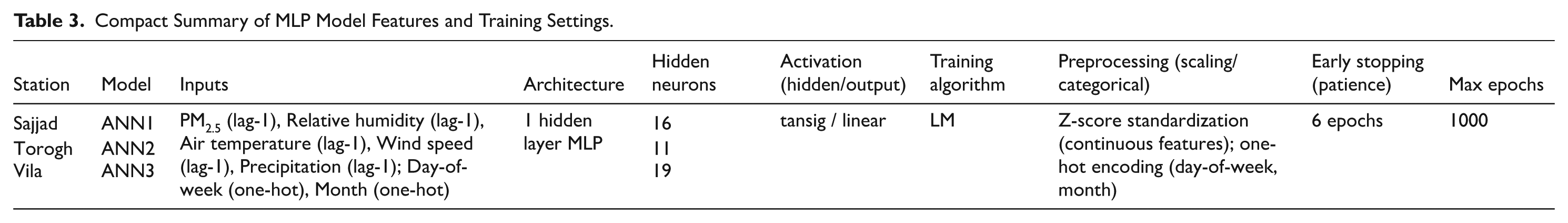
The variation in the optimal number of neurons across the stations can be attributed to the distinct statistical characteristics of each dataset. Factors such as data variance and coefficient of variation, the presence of nonlinear patterns of varying complexity, and the signal-to-noise ratio at each station significantly influence the model capacity required for effective learning. Specifically, stations like Vila, which exhibit more severe fluctuations or more complex temporal patterns in PM_2.5 concentrations, require a larger number of neurons in the hidden layer to adequately capture the intrinsic structure of the data. This finding underscores that the optimal neural network architecture cannot be uniform or universally applied across all datasets; rather, it must be individually determined based on the statistical properties and inherent complexity of the data at each location. In this context, the trade-off between bias and variance is particularly important. Increasing the number of neurons enhances model capacity, which may reduce bias but increase variance, potentially leading to overfitting. Conversely, too few neurons may result in high bias and underfitting. Therefore, determining the optimal number of neurons should strike a balance between these 2 factors, ensuring that the model maintains sufficient generalization capability while accurately capturing complex data patterns.³⁶

Neural Network Performance

The performance of the neural network at the 3 air quality monitoring stations in Mashhad—Sajjad, Torogh, and Vila—is illustrated in Figure 3. This figure presents the statistical performance indicators for the training, validation, and testing phases. Based on these results, the model exhibited strong learning capability during the training phase and maintained satisfactory performance in both the validation and testing stages. These findings demonstrate the model’s adequate generalization ability in predicting PM_2.5 concentrations for unseen data.

Figure 3.

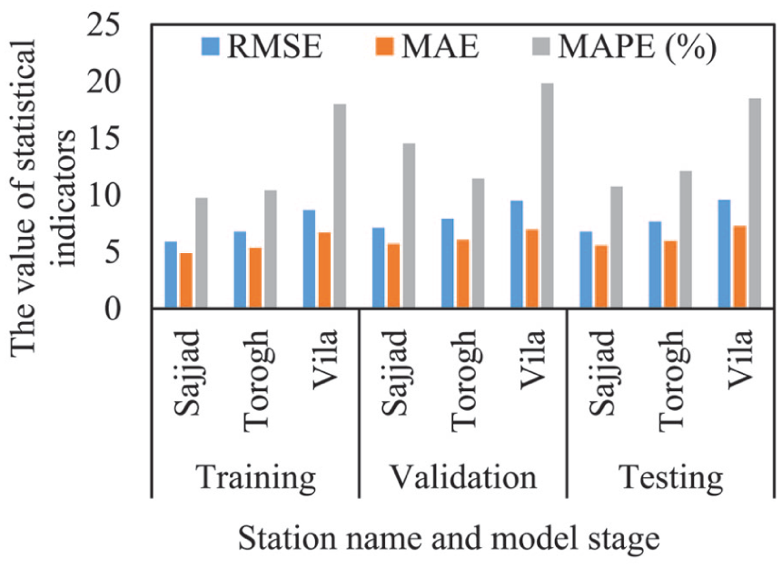
Comparison of MLP model performance indicators during the training, validation, and testing phases at the 3 monitoring stations.

The Sajjad station, located in 1 of the most traffic-congested urban areas of Mashhad, demonstrated the highest predictive performance. This outcome can be attributed to the relatively stable pattern of traffic-related pollution, spatial and temporal consistency in pollutant dispersion, and the absence of diverse or complex emission sources. The model’s statistical performance during the testing phase at this station included an R² of .79, an RMSE of 6.77 µg/m³, a Mean Absolute Error (MAE) of 5.54 µg/m³, and a Mean Absolute Percentage Error (MAPE) of approximately 10.73%, indicating good agreement between observed and predicted concentrations.

At the Torogh station, despite its peripheral location, high pollution levels were recorded—primarily due to industrial activities, the movement of heavy-duty diesel vehicles, soil erosion, and transboundary pollutant transport from neighboring regions. In this case, the model achieved a testing-phase R² of .78, an RMSE of 7.65 µg/m³, an MAE of 5.94 µg/m³, and a MAPE of approximately 12.09%. Although the predictive accuracy at Torogh was slightly lower than at Sajjad, the model’s performance remains within an acceptable range.³⁷

The Vila station, located in a moderately urbanized area near the Binalood mountain range, exhibited the weakest performance in predicting daily PM_2.5 concentrations. Nevertheless, even at this station, the model demonstrated an acceptable ability to capture the general data patterns. During the testing phase, the statistical indicators included an R² of .65, an RMSE of 9.56 µg/m³, an MAE of 7.24 µg/m³, and a MAPE of approximately 18.49%.

The reduced accuracy at this station can be attributed to the high spatiotemporal variability of multiple pollution sources—such as dispersed residential, commercial, and traffic-related activities—which, unlike the Sajjad and Torogh stations, lack spatial and temporal coherence. Furthermore, the station’s geographical location near mountainous terrain influences the formation of meteorological phenomena such as temperature inversions, regional airflows, and specific wind patterns. These factors lead to reduced atmospheric stability and nonlinear pollutant transport, thereby complicating accurate prediction. The interplay of these conditions has diminished the model’s capacity to precisely simulate pollutant concentration behavior in this area.

Figure 4 illustrates the regression results between observed and predicted daily PM_2.5 concentrations for the training, validation and test phases. Each subplot (a-i) is annotated with R², RMSE (µg/m³), MAE (µg/m³) and the number of samples (n). As shown, a strong correlation between observed and predicted values is evident at all 3 monitoring stations.

Figure 4.

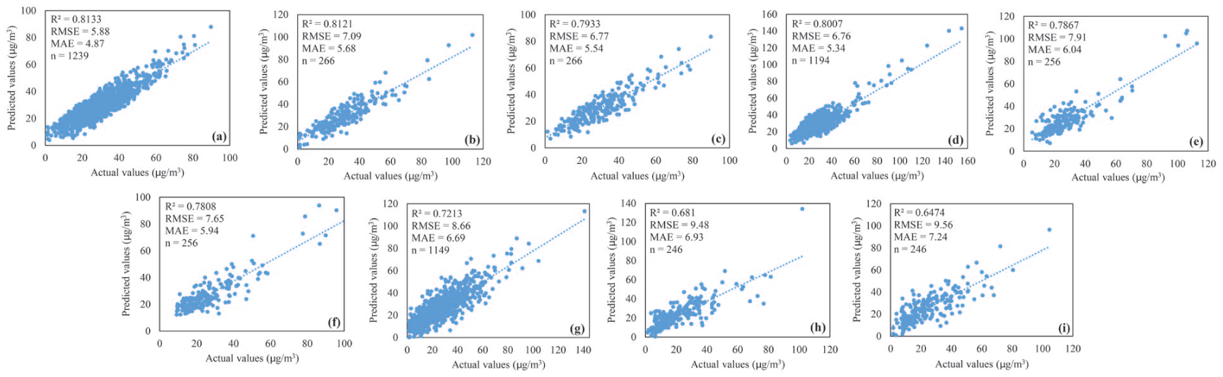
Regression plots comparing the actual and predicted daily PM_2.5 concentrations using the MLP neural network model at the 3 monitoring stations. Sajjad Station—(a) training data, (b) validation data, (c) testing data; Torogh Station—(d) training data, (e) validation data, (f) testing data; Vila Station—(g) training data, (h) validation data, (i) testing data. Each subplot reports R², RMSE, MAE, and the number of data points (n).

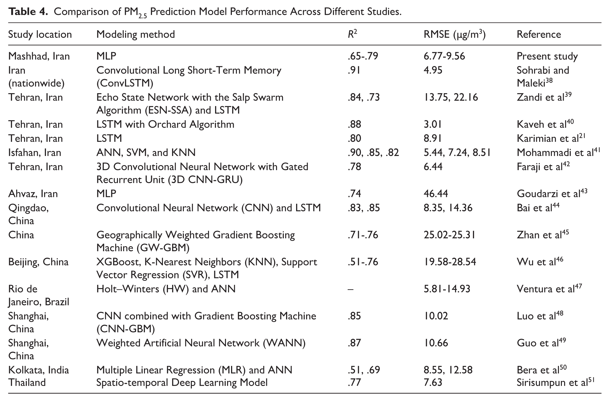
Based on the results presented in Figures 3 and 4, the neural network model demonstrated higher accuracy in areas with more consistent pollution patterns, such as the Sajjad station, while its performance declined in regions characterized by diverse pollution sources or distinct climatic conditions. For further validation, the findings of this study were compared with those of previous research, as summarized in Table 4, which corroborates the accuracy and effectiveness of the modeling approach employed in the present study.

Table 4.

Comparison of PM_2.5 Prediction Model Performance Across Different Studies.

Study location	Modeling method	R ²	RMSE (µg/m³)	Reference
Mashhad, Iran	MLP	.65-.79	6.77-9.56	Present study
Iran (nationwide)	Convolutional Long Short-Term Memory (ConvLSTM)	.91	4.95	Sohrabi and Maleki³⁸
Tehran, Iran	Echo State Network with the Salp Swarm Algorithm (ESN-SSA) and LSTM	.84, .73	13.75, 22.16	Zandi et al³⁹
Tehran, Iran	LSTM with Orchard Algorithm	.88	3.01	Kaveh et al⁴⁰
Tehran, Iran	LSTM	.80	8.91	Karimian et al²¹
Isfahan, Iran	ANN, SVM, and KNN	.90, .85, .82	5.44, 7.24, 8.51	Mohammadi et al⁴¹
Tehran, Iran	3D Convolutional Neural Network with Gated Recurrent Unit (3D CNN-GRU)	.78	6.44	Faraji et al⁴²
Ahvaz, Iran	MLP	.74	46.44	Goudarzi et al⁴³
Qingdao, China	Convolutional Neural Network (CNN) and LSTM	.83, .85	8.35, 14.36	Bai et al⁴⁴
China	Geographically Weighted Gradient Boosting Machine (GW-GBM)	.71-.76	25.02-25.31	Zhan et al⁴⁵
Beijing, China	XGBoost, K-Nearest Neighbors (KNN), Support Vector Regression (SVR), LSTM	.51-.76	19.58-28.54	Wu et al⁴⁶
Rio de Janeiro, Brazil	Holt–Winters (HW) and ANN	–	5.81-14.93	Ventura et al⁴⁷
Shanghai, China	CNN combined with Gradient Boosting Machine (CNN-GBM)	.85	10.02	Luo et al⁴⁸
Shanghai, China	Weighted Artificial Neural Network (WANN)	.87	10.66	Guo et al⁴⁹
Kolkata, India	Multiple Linear Regression (MLR) and ANN	.51, .69	8.55, 12.58	Bera et al⁵⁰
Thailand	Spatio-temporal Deep Learning Model	.77	7.63	Sirisumpun et al⁵¹

Model Performance Evaluation in Predicting Daily PM_2.5 Exceedances

To assess the performance of a prediction system, various evaluation metrics can be employed. One of the most critical indicators is the system’s ability to accurately predict exceedances of the daily air quality standard. According to the Iranian National Ambient Air Quality Standard, the permissible daily limit for PM_2.5 is set at 35 µg/m³.⁵

To analyze the model’s effectiveness in forecasting exceedance events, 3 key statistical indicators were used: True Positive Rate (TPR), False Alarm Rate (FAR), and F1-score. These metrics were calculated by comparing the predicted values against observed data for instances where daily PM_2.5 concentrations exceeded the threshold of 35 µg/m³.

The parameters used to compute these performance indicators include: A, the number of correctly predicted exceedance events; F, the total number of predicted exceedances (both true and false); M, the total number of actual exceedance events; and N, the total number of days analyzed (ie, total data points). In this context, the ratio of true positive predictions to all predicted exceedances (A/F) represents the precision of the model in identifying exceedance cases.

The TPR, as defined in equation (2), reflects the model’s ability to correctly identify days with actual exceedances and is considered a measure of the model’s sensitivity.

T P R = \frac{A}{M}

(2)

The FAR, as defined in equation (3), indicates the proportion of predicted exceedance events that did not actually exceed the threshold.

F A R = \frac{F - A}{F}

(3)

The F1-score (equation (4)) represents the harmonic mean of precision and sensitivity (TPR). This metric is particularly useful in imbalanced classification problems, where the number of exceedance and non-exceedance cases are unevenly distributed. The F1-score effectively balances the model’s ability to correctly detect exceedances while minimizing false alarms. A value closer to 1 indicates superior model performance. In environmental applications, F1-scores greater than 0.70 are typically considered acceptable.

F 1 - S c o r e = \frac{2 \cdot P r e c i s i o n \cdot T P R}{P r e c i s i o n + T P R}

(4)

Table 5 presents the performance metrics of the ANN model in predicting exceedance events of the daily PM_2.5 threshold (35 µg/m³) at 3 air quality monitoring stations in Mashhad during the period 2018 to 2023. The results indicate notable spatial differences in model performance. Specifically, the ANN model demonstrated superior predictive accuracy at the Sajjad station, while a marked decline in performance was observed at the Vila station.

Table 5.

Performance Metrics of the ANN Model for Predicting Daily PM_2.5 Exceedance Events (>35 µg/m³) at Air Quality Monitoring Stations in Mashhad.

Station	N (total days)	M (observed exceedances)	F (predicted exceedances)	A (true positives)	TPR	FAR	F1-score
Sajjad	1771	463	421	343	0.74	0.18	0.78
Torogh	1706	225	198	159	0.71	0.19	0.75
Vila	1641	323	295	211	0.66	0.28	0.68

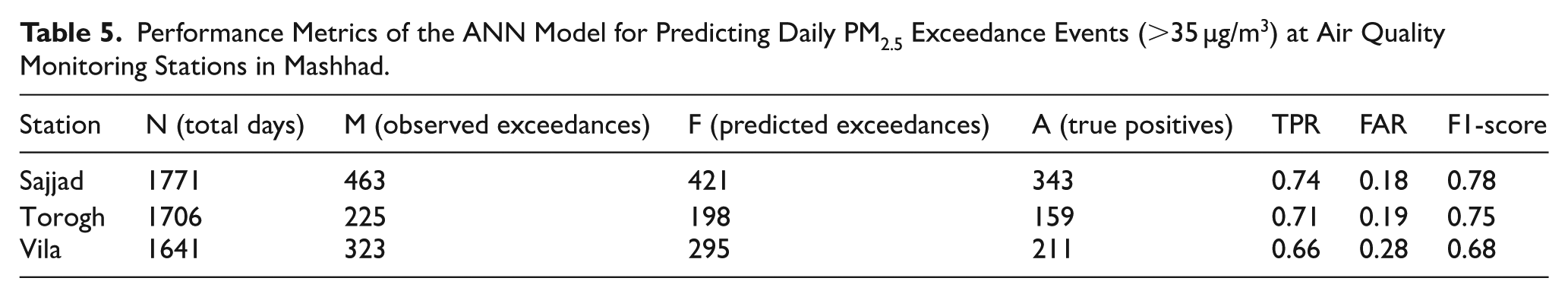
At the Sajjad monitoring station, the model’s performance indicators demonstrate considerable success in identifying pollution events characterized by daily PM_2.5 concentrations exceeding the regulatory threshold. A TPR of 0.74 indicates that 74% of actual exceedance events were correctly identified. Moreover, a FAR of 0.18 reflects the model’s ability to minimize false positive predictions. The F1-score, a composite metric balancing precision and recall, was calculated as 0.78, indicating a favorable balance between sensitivity and precision in detecting critical pollution events. The model’s superior performance at the Sajjad station can be attributed to the relatively lower density of unpredictable pollution sources—such as construction activities and episodic public events—which often reduce forecasting accuracy. Additionally, the relative consistency of pollution patterns in this area likely enhances the model’s generalizability.

The ANN model’s performance in predicting PM_2.5 exceedance events aligns well with findings from similar studies conducted in regions characterized by stable pollution patterns. For instance, F1-scores ranging from 0.77 to 0.88 have been reported in Isfahan⁴¹; an F1-score of 0.62 was observed in Jakarta⁵²; and TPR values between 60% and 75% were documented in the western United States.⁵³ Furthermore, in Athens, the TPR and FAR were reported as approximately 0.78 and 17.9%, respectively.⁵⁴

The Torogh monitoring station, located on the southeastern outskirts of Mashhad and adjacent to industrial zones, exhibited relatively stable performance comparable to that of the Sajjad station. The F1-score and FAR at this station were calculated as 0.75 and 0.19, respectively, indicating acceptable accuracy in predicting pollution events and a low rate of false alarms. The presence of relatively consistent pollution patterns stemming from industrial activities, along with the spatial distance from the city center—which reduces the diversity of pollution sources—are key factors contributing to reduced data noise and improved model performance. The findings of this study are consistent with results reported in other industrial regions. For instance, ANN models achieved F1-scores of approximately 0.76 in the Shah Alam Industrial Area, Malaysia,⁵⁵ and F1-scores ranging from 0.74 to 0.80 in the Puli Industrial Zone in Taiwan.⁵⁶

In contrast, at the Vila station, the F1-score dropped to 0.68, indicating a decline in model performance. This station is situated in the southwestern part of Mashhad, in an area characterized by specific topographic features, including proximity to southern highlands and urban green spaces. Such conditions cause significant variability in wind flow and pollution dispersion patterns. Furthermore, temperature inversion phenomena—especially during early morning hours or colder seasons—can lead to the accumulation of pollutants in the lower atmospheric layers, complicating their dispersion patterns. These dynamics are often overlooked in models that lack vertical atmospheric data. Additionally, the meteorological data used in the modeling process were derived from synoptic stations, which mainly provide generalized representations of regional atmospheric conditions and are insufficient for capturing fine-scale local variations. This mismatch between input data and real-world conditions has likely reduced the model’s predictive accuracy at this station.

Therefore, the integration of high-resolution mesoscale meteorological models, such as the Weather Research and Forecasting (WRF) model, can enhance the accuracy of local input data—particularly in regions with complex terrain and heterogeneous climatic conditions—thereby improving prediction performance. Similar studies have also highlighted the adverse effects of topographical complexity and climatic variability on the performance of air pollution forecasting models. For example, research conducted in Thailand⁵⁰ and India⁵¹ reported that in mountainous or valley regions, ANN models experienced significant performance declines, with mean F1-scores ranging between 0.58 and 0.65. These findings are consistent with the performance observed at the Vila station.

Overall, the analysis of Table 5 reveals that the ANN model performs significantly better at stations located in areas with well-defined emission sources, stable dispersion patterns, and relatively simple topographic conditions. This underscores the importance of spatial adaptability in model design, the necessity of high-resolution meteorological data, and the inclusion of local geographic characteristics in the development of air quality forecasting and early warning systems. Given the model’s satisfactory performance at selected stations, it can serve as a foundational component for the implementation of localized air pollution alert systems.

Conclusions

The results of this study indicate that MLP neural network models, when individually designed and optimized for each monitoring site, can provide reliable next-day PM_2.5 forecasts across different urban and semi-industrial environments. Quantitatively, the final models achieved test-phase performance as follows: Sajjad—R² = .79, RMSE = 6.77 µg/m³, MAE = 5.54 µg/m³ (n = 266); Torogh—R² = .78, RMSE = 7.65 µg/m³, MAE = 5.94 µg/m³ (n = 256); Vila—R² = .65, RMSE = 9.56 µg/m³, MAE = 7.24 µg/m³ (n = 246). These results reflect higher predictive accuracy at sites with more homogeneous emission sources and stable dispersion patterns (Sajjad), and lower accuracy at locations with complex topography and more variable source contributions (Vila).

The applied preprocessing and training choices substantially contributed to model performance: input features were standardized (z-score), temporal categorical variables were one-hot encoded, early stopping (patience = 6 epochs) was used, and network architectures were optimized per site (16 hidden neurons for Sajjad, 11 for Torogh, and 19 for Vila). Feature selection based on correlation analysis supported the inclusion of air temperature, relative humidity, and average wind speed as the most influential predictors, whereas wind direction and solar radiation showed negligible predictive value and were excluded to reduce multicollinearity and simplify the models.

Taken together, these findings demonstrate that properly configured MLPs can serve as effective components of localized air-quality forecasting and early-warning systems. For operational deployment and further improvement, recommended next steps include increasing the spatial resolution of meteorological inputs, testing alternative deep-learning architectures at sites with strong temporal variability, and maintaining ongoing model validation with updated observational datasets.

Footnotes

Acknowledgements

The authors would like to thank the Khorasan Razavi Meteorological Organization (Iran) for providing access to meteorological data used in this study. We also gratefully acknowledge the Khorasan Razavi Department of Environment (Iran) for supplying the PM2.5 concentration data. This research was conducted during a sabbatical leave as part of the Faculty–Industry and Society Collaboration Program, and the authors appreciate the support of the University of Birjand (Iran) in this regard.

ORCID iD

Mohamad Javad Zoqi

Author Contributions

Conceptualization, MJZ; methodology, MJZ and ADA; software, MJZ; validation, MJZ and SJR; formal analysis, MJZ; investigation, MJZ; data curation, MJZ and ADA; writing—original draft preparation, MJZ; writing—review and editing, MJZ, ADA, SJR and MRMD; visualization, MJZ; supervision, MRMD; project administration, MJZ; resources, ADA and SJR. All authors have read and approved the final manuscript.

Funding

The authors received no financial support for the research, authorship, and/or publication of this article.

Declaration of Conflicting Interests

The authors declared no potential conflicts of interest with respect to the research, authorship, and/or publication of this article.

Data Availability Statement

The dataset and MATLAB code used in this study are available in the Zenodo repository at: . This includes MATLAB scripts for data preprocessing, neural network training, and performance evaluation.

References

Biswal

Bolan

Zhu

Y-G

Balasubramanian

Nature-based systems (NbS) for mitigation of stormwater and air pollution in urban areas: a review. Resour Conserv Recycl. 2022;186:106578.

Guo

Wang

Prediction of monthly PM2.5 concentration in Liaocheng in China employing artificial neural network. Atmos. 2022;13(8):1221.

Yang

Wang

Huang

Kelly

Long-term exposure to multiple ambient air pollutants and association with incident depression and anxiety. JAMA Psychiatr. 2023;80(4):305-313.

WHO. WHO Global Air Quality Guidelines: Particulate Matter (PM2. 5 and PM10), Ozone, Nitrogen Dioxide, Sulfur Dioxide and Carbon Monoxide. World Health Organization; 2021.

Ambient Air Quality Standards (Approval No. 19322 of the Supreme Council for Environmental Protection . Monitoring and Assessment Office, Deputy for Human Environment; 2016.

Guo

Wang

, et al Changes in air quality from the COVID to the post-COVID era in the Beijing-Tianjin-Tangshan region in China. Aerosol Air Qual Res. 2021;21(12):210270.

Guo

Wang

A hybrid wavelet-based deep learning model for accurate prediction of daily surface PM(2.5) concentrations in Guangzhou City. Toxics. 2025;13(4):254.

Karimian

, et al Daily estimation of fine particulate matter mass concentration through satellite based aerosol optical depth. ISPRS Ann Photogramm Remote Sens Spat Inf Sci. 2017;4:175-181.

Shahsavani

Tobías

Querol

, et al Short-term effects of particulate matter during desert and non-desert dust days on mortality in Iran. Environ Int. 2020;134:105299.

10.

Etemad-Shahidi

Zoghi

Saeedi

An alternative data driven approach for prediction of thermal discharge initial dilution using tee diffusers. Int J Environ Sci Technol. 2010;7:29-36.

11.

Guo

, et al Air pollution forecasting using artificial and wavelet neural networks with meteorological conditions. Aerosol Air Qual Res. 2020;20(6):1429-1439.

12.

Shams

Kalantary

Jahani

, et al Assessing the effectiveness of artificial neural networks (ANN) and multiple linear regressions (MLR) in forcasting AQI and PM10 and evaluating health impacts through AirQ+ (case study: Tehran). Environ Pollut. 2023;338:122623.

13.

Cakir

Sita

Evaluating the performance of ANN in predicting the concentrations of ambient air pollutants in Nicosia. Atmos Pollut Res. 2020;11(12):2327-2334.

14.

Boznar

Lesjak

Mlakar

A neural network-based method for short-term predictions of ambient SO2 concentrations in highly polluted industrial areas of complex terrain. Atmos Environ B Urban Atmos. 1993;27(2):221-230.

15.

Guo

Comparative analysis of multiple deep learning models for forecasting monthly ambient PM2.5 concentrations: a case study in Dezhou City, China. Atmos. 2024;15(12):1432.

16.

Guo

Wang

Assessing the effectiveness of long short-term memory and artificial neural network in predicting daily ozone concentrations in Liaocheng City. Sci Rep. 2025;15(1):6798.

17.

Elbayoumi

Ramli

Fitri

Yusof

NF.

Development and comparison of regression models and feedforward backpropagation neural network models to predict seasonal indoor PM2.5–10 and PM2.5 concentrations in naturally ventilated schools. Atmos Pollut Res. 2015;6(6):1013-1023.

18.

Suri

Jain

Kapoor

, et al Air quality prediction-a study using neural network based approach. J Soft Comput Civil Eng. 2023;7(1):93-113.

19.

Yang

M-C

Chen

MC.

Composite neural network: theory and application to PM2.5 prediction. IEEE Trans Knowl Data Eng. 2021;35(2):1-1323.

20.

Ganesh

Arulmozhivarman

Tatavarti

VSNR

. Prediction of PM2.5 using an ensemble of artificial neural networks and regression models. J Ambient Intell Humaniz Comput. Published online April 30, 2018;1-11. doi:10.1007/s12652-018-0801-8

21.

Karimian

, et al Evaluation of different machine learning approaches to forecasting PM2.5 mass concentrations. Aerosol Air Qual Res. 2019;19(6):1400-1410.

22.

Daneshvar

MRM

Rahmati

Rasouli

Aliaqa

. An analysis of the spatial and temporal correlations between rainfall events and earth surface characteristics, Mashhad district in northeastern Iran. Theor Appl Climatol. 2025;156(2):1-18.

23.

Mohammadi

Hatami

Esmaeli

Gohari

Mohammadi

Khayami

Relationships between ambient air pollution, meteorological parameters and respiratory mortality in Mashhad, Iran: a time series analysis. Pollution. 2022;8(4):1250-1265.

24.

Shukla

Aggarwal

SG.

A technical overview on beta-attenuation method for the monitoring of particulate matter in ambient air. Aerosol Air Qual Res. 2022;22(12):220195.

25.

Zoqi

MJ.

Generalization of artificial neural network for predicting methane production in laboratory-scale anaerobic bioreactor landfills. Global J Environ Sci Manag. 2024;10(1):225-244.

26.

Cheng

Sun

Yao

Cao

A variable selection method based on mutual information and variance inflation factor. Spectrochim Acta Part A Molec Biomol Spectr. 2022;268:120652.

27.

Emekwuru

Ejohwomu

Temperature, humidity and air pollution relationships during a period of rainy and dry seasons in Lagos, West Africa. Climate. 2023;11(5):113.

28.

Nyayapathi

Namuduri

Kolli

SK.

A comprehensive review of vertical profiling of ambient air quality-particulate matter and its impacts on climatic & environmental health. Air Qual Atmos Health. 2025;18:1569-1595.

29.

Liu

, et al The relationship between atmospheric boundary layer and temperature inversion layer and their aerosol capture capabilities. Atmos Res. 2022;271:106121.

30.

Mansouri Daneshvar

Khatami

Ebrahimi

An analysis of urban heat island based on the temperature inversion across the atmospheric boundary layer in Mashhad, Iran (2018–2022). Spat Inf Res. 2024;32(5):607-622.

31.

Guo

Wang

The characteristics of air quality changes in Hohhot City in China and their relationship with meteorological and socio-economic factors. Aerosol Air Qual Res. 2024;24(5):230274.

32.

Marzouni

Alizadeh

Banafsheh

, et al A comparison of health impacts assessment for PM10 during two successive years in the ambient air of Kermanshah, Iran. Atmos Pollut Res. 2016;7(5):768-774.

33.

Karimian

, et al Spatio-temporal variation of wind influence on distribution of fine particulate matter and its precursor gases. Atmos Pollut Res. 2019;10(1):53-64.

34.

Zhao

Liu

Vanos

Cao

Day-of-week and seasonal patterns of PM2.5 concentrations over the United States: time-series analyses using the Prophet procedure. Atmos Environ. 2018;192:116-127.

35.

Guo

Wang

Monthly climate prediction using deep convolutional neural network and long short-term memory. Sci Rep. 2024;14(1):17748.

36.

Guo

Wang

Prediction of hourly PM2.5 and PM10 concentrations in Chongqing City in China based on artificial neural network. Aerosol Air Qual Res. 2023;23(6):220448.

37.

Gulati

Bansal

Pal

Mittal

Sharma

Gared

Estimating PM(2.5) utilizing multiple linear regression and ANN techniques. Sci Rep. 2023;13(1):22578.

38.

Sohrabi

Maleki

Fusing satellite imagery and ground-based observations for PM(2.5) air pollution modeling in Iran using a deep learning approach. Sci Rep. 2025;15(1):21449.

39.

Zandi

Jafari

Lotfata

Enhancing PM2.5 air pollution prediction performance by optimizing the Echo State Network (ESN) deep learning model using new metaheuristic algorithms. Urban Sci. 2025;9(5):138.

40.

Kaveh

Mesgari

Kaveh

A novel evolutionary deep learning approach for PM2.5 prediction using remote sensing and spatial–temporal data: a case study of Tehran. ISPRS Int J Geo Inf. 2025;14(2):42.

41.

Mohammadi

Teiri

Hajizadeh

Abdolahnejad

Ebrahimi

Prediction of atmospheric PM(2.5) level by machine learning techniques in Isfahan, Iran. Sci Rep. 2024;14(1):2109.

42.

Faraji

Nadi

Ghaffarpasand

Homayoni

Downey

An integrated 3D CNN-GRU deep learning method for short-term prediction of PM2.5 concentration in urban environment. Sci Total Environ. 2022;834:155324.

43.

Goudarzi

Hopke

Yazdani

Forecasting PM(2.5) concentration using artificial neural network and its health effects in Ahvaz, Iran. Chemosphere. 2021;283:131285.

44.

Bai

Zhang

Cao

Chen

Prediction of PM(2.5) concentration based on a CNN-LSTM neural network algorithm. PeerJ. 2024;12:e17811.

45.

Zhan

Luo

Deng

, et al Spatiotemporal prediction of continuous daily PM2.5 concentrations across China using a spatially explicit machine learning algorithm. Atmos Environ. 2017;155:129-139.

46.

Lin

Shi

Fang

Seasonal prediction of daily PM2.5 concentrations with interpretable machine learning: a case study of Beijing, China. Environ Sci Pollut Res. 2022;29(30):45821-45836.

47.

Ventura

LMB

de Oliveira Pinto

Soares

Luna

Gioda

. Forecast of daily PM2.5 concentrations applying artificial neural networks and Holt–Winters models. Air Qual Atmos Health. 2019;12:317-325.

48.

Luo

Huang

Liu

PM2.5 concentration estimation using convolutional neural network and gradient boosting machine. J Environ Sci. 2020;98:85-93.

49.

Guo

Wang

Predicting of daily PM(2.5) concentration employing wavelet artificial neural networks based on meteorological elements in Shanghai, China. Toxics. 2023;11(1):51.

50.

Bera

Bhattacharjee

Sengupta

Saha

PM(2.5) concentration prediction during COVID-19 lockdown over Kolkata metropolitan city, India using MLR and ANN models. Environ Chall. 2021;4:100155.

51.

Sirisumpun

Wongwailikhit

Painmanakul

Vateekul

Spatio-temporal PM2.5 forecasting in Thailand using encoder-decoder networks. IEEE Access. 2023;11:69601-69613.

52.

Marsha

Larkin

NK.

A statistical model for predicting PM_2.5 for the western United States. J Air Waste Manag Assoc. 2019;69(10):1215-1229.

53.

Moustris

Ziomas

Paliatsos

AG.

3-Day-ahead forecasting of regional pollution index for the pollutants NO2, CO, SO2, and O3 using artificial neural networks in Athens, Greece. Water Air Soil Pollut. 2010;209:29-43.

54.

Toharudin

Caraka

Pratiwi

, et al Boosting algorithm to handle unbalanced classification of PM_2.5 concentration levels by observing meteorological parameters in Jakarta-Indonesia using AdaBoost, XGBoost, CatBoost, and LightGBM. IEEE Access. 2023;11:35680-35696.

55.

Arafin

Ul-Saufie

Md Ghani

Ibrahim

A two-stage feature selection method to enhance prediction of daily PM2.5 concentration air pollution. Environ Nat Resour J. 2024;22(6):1-10.

56.

Yin

P-Y

Chang

R-I

Day

R-F

Lin

Y-C

CY.

Improving PM2.5 concentration forecast with the identification of temperature inversion. Appl Sci. 2021;12(1):71.

Prediction of Daily PM 2.5 Concentrations Using Neural Networks at 3 Urban Monitoring Stations With Diverse Land Uses

Abstract

Plain Language Summary

Keywords

Introduction

Materials and Methods

Design and Training of MLP Neural Networks

Study Area

Data Preparation

Input Variables

Results

Correlation Analysis Between Input Variables and PM2.5 Concentration

Neural Network Structure

Neural Network Performance

Model Performance Evaluation in Predicting Daily PM2.5 Exceedances

Conclusions

Footnotes

Acknowledgements

ORCID iD

Author Contributions

Funding

Declaration of Conflicting Interests

Data Availability Statement

References

Correlation Analysis Between Input Variables and PM_2.5 Concentration

Model Performance Evaluation in Predicting Daily PM_2.5 Exceedances