Sage Journals: Discover world-class research

Abstract

The Loess Plateau of China is facing increasingly serious challenges related to water shortage issues despite the successful vegetation restoration. Surface soil water (0–40 cm) is crucial to water transfer and discharge in the soil-plant-atmosphere continuum, which is controlled by precipitation (P), air temperature (T_a), and plant components. This study selected one typical grass species and set different treatments of natural condition (NC), removing litter (CR), and only roots (OR), to analyze the responses of soil water storage (W) and its change (∆W) to P and T_a at different time scales (including daily, weekly and monthly scales). The results showed that P had significantly positive effects on W and ∆W, while T_a negatively influenced W and ∆W. Meanwhile, T_a also controlled the significance of P affecting W. P contributed more (53–63%) to ∆W variation at the daily scale, but T_a showed more effect (73–80%) at the weekly scale, and both of them contributed more than 77% at the monthly scale. P and T_a existed a threshold phenomenon for increasing soil water, where P thresholds were higher than 0.93, 4.98, and 28.17 mm and Ta threshold were lower than 28.69, 28.89, and 29.96°C at the daily, weekly and monthly scales, respectively. Moreover, grass components also affected the responses of ∆W to P and T_a, and the OR treatment displayed the lowest sensitivity and had the lowest loss rate of soil water. The total infiltration, total loss amount, and rainwater retention rate exhibited: NC > CR > OR. Overall, grass canopy and litter improved soil water condition, and the roots most strongly protected soil water after infiltration. This study can provide a better understanding of surface soil water responding to climate change under drought stress with water shortage implications, and may strength the management of grassland in semi-arid region.

Keywords

Rainfall threshold soil moisture soil hydrological processes grassland restoration temporal scales

Introduction

The Loess Plateau of China is well-known for the successful implementation of Grain-for-Green Project in 1999, which aimed to restore vegetation but also led to severe water shortage challenges currently (Fu et al., 2017; Yu et al., 2020). The extensive vegetation restoration has significantly depleted soil water, resulting in the formation and strengthening of the soil dried layer in the Loess Plateau (Han et al., 2022; Wang et al., 2011). Soil water storage (W) is a crucial factor used to evaluate soil water conservation after vegetation restoration. The change in soil water storage (∆W) at a shallow soil depth (0–40 cm) is primarily affected the input processes (such as rainfall infiltration) and output processes (such as evapotranspiration (ET), including plant transpiration, canopy interception and soil water evaporation) (Fang et al., 2019; Wang et al., 2013). These processes are influenced by factors such as the climate change (including precipitation and air temperature) as well as surface coverage (Jin et al., 2018; Ramos et al., 2008).

Soil water is only replenished by precipitation (P) due to the thickness soil layers and fragmented topographic landscapes. Many studies have investigated the relationships between P and soil water, most focusing on the effect of rainfall intensity, duration, amount and different patterns at the event scale (Du et al., 2019; Ge et al., 2022; He et al., 2020; Jin et al., 2018; Yu et al., 2022; Zhang et al., 2016; Zhao et al., 2022). However, the temporal response of soil water to P at different time scales remained unclear. In most cases, the maximum infiltration depth of soil during a rainfall event was 40 cm (Chen et al., 2020; Du et al., 2019; Jin et al., 2018; Wang et al., 2013), emphasizing the importance of the surface W to respond to P. Generally, when P dropped, the W would increase due to the replenishment effects. However, soil water may not increase or even the ∆W could be negative, when the P amounts were lower than 2 to 7 mm (Dai & Wang, 2021; Ge et al., 2022; Liu et al., 2023), due to the interception from vegetation and consumption of ET. Moreover, the delayed effect of rainfall infiltration on soil water was difficult to determine at shorter time scales (Dai & Wang, 2021), which could be considered by the cumulative effects of infiltration processes at the longer time scale.

Air temperature (T_a) is an essential meteorological factor that mainly affects evapotranspiration (ET) processes, ultimately controlling soil water consumption (Ramos et al., 2008). ET is the process that drives the upward movement of soil water (Longobardi & Khaertdinova, 2015), resulting in the depletion of soil water. Soil water demands increased 6–14% if T_a increased by 1°C due to the shorter-term change of ET in the growing season (Ramos et al., 2008). The long-term heat accumulation controlled by T_a had a continuous effect on ET as well as soil water (Jiao et al., 2016; Liu & Zhang, 2013; Longobardi & Khaertdinova, 2015; Ramos et al., 2008). However, the direct contribution of T_a to soil water is still unclear, and combining the effect of P and T_a could help improve our understanding of soil water response to climate change, which is the objective of this study.

Plant components (including canopy, litter, and roots) have been proven to play an important role in hydrologic cycle processes, such as rainfall redistribution, runoff, infiltration, evaporation, and transpiration (Allen et al., 2014; Liu et al., 2018; Qiu et al., 2023; Tanaka & Hashimoto, 2006; Wang et al., 2022b; Wu et al., 2017), and then to influence soil water conservation. Good et al. (2015) studied the strong effects of vegetation on soil hydrological processes at the global scale, and found that transpiration might account for approximate 64% of the total ET, and soil water originally provided about 65% of evaporation. The canopy firstly intercepts precipitation to start the hydrological process, and consumes soil water through the transpiration process at the same time (Allen et al., 2014; Qiu et al., 2023; Tanaka & Hashimoto, 2006). The litter also had some function in the interception process, and more function in preventing soil evaporation and disturbing runoff and infiltration processes (Liu et al., 2018; Xiong et al., 2008; Zhao et al., 2022). The roots are well recognized to have a function of promoting soil water infiltration (Liu et al., 2018; Wang et al., 2022b; Wu et al., 2017). The grass components could change the response of runoff to rainfall regimes, and grass canopy cover had the lowest runoff coefficient but higher subsurface flow rate in the red soil region, with the highest subsurface flow rate occurring in litter cover (Liu et al., 2016).

The function of soil water in the soil-plant-atmosphere continuum is significantly affected by climate change (e.g., P and T_a), and the change mechanism needs more study at different time scales. So, we would display the synergic relationship between P and T_a, to reflect the degree of meteorological change during the whole observation period in 2015. On this basic, our purposes of this study were to analyze the temporal dynamics of W with the change of P and T_a at different time scales, quantify the contribution and relative influences of P and T_a on W and ∆W, and evaluate the roles of grass components in soil water retention/loss rates.

Materials and Methods

Study area

Yangjuangou catchment (36°42′N, 109°31′E) is a typical hilly and gully catchment in the Loess Plateau of China (Figure 1). The elevation of the studied catchment ranges from 1,050 to 1,298 m with a total area of 2.02 km². The average annual P is 536 mm ranging from 330 to 959 mm during 1951 to 2016, which is mainly concentrated between June and September, accounting for more than 70% of total annual P, with large inter-annual variations. The average annual T_a is 9.4°C (Liu et al., 2022). The soil is a Calcaric Cambisol with a maximum depth of approximately 200 m. The Grain-for-Green project has been applied in this catchment since 1999, and the effect of vegetation restoration is very significant. Grass land becomes the main land use type since the application of this project, where Andropogon yunnanensis is one of the predominant herb species.

Figure 1.

Location of the study area and the plots with different treatments. NC showed the natural condition including canopy, litter and roots of grass. CR showed canopy + roots with removing litter.

Field experiments

The typical grass species (Andropogon yunnanensis) was selected to monitor the dynamic of soil water. Three types of treatments were set in the grassland slope, including (1) NC treatment: the natural condition without any artificial disturbance; (2) CR treatment: the canopy+roots, namely removing the litter; (3) OR treatment: only roots with removing both of canopy and litter. The microplots were established for each treatment with three repeats, in order to avoid effects of surrounding surface runoff and subsurface flow. Each plot had a boundary consisting of PVC and plastic material sheets (50 cm depth), with a size of 0.8 m × 0.8 m. The slope gradient was approximately 21° and the slope aspect was northeast.

We installed EC-5 sensors to measure the volumetric soil water content (SWC, m³/m³) at 5, 10, 20, and 40 cm depths in three plots for each treatment type. Soil water was recorded at 5 min intervals by the data logger (U30, Onset Computer Corp., Bourne, MA, USA). Precipitation (P, mm) was measured by a tipping bucket rain gauge (RG3-M, Onset Computer Corp., Bourne, MA, USA) with the resolution of 0.2 mm. The rain gauge was placed in an open area near microplots. Air temperature (T_a, °C) was monitored by an automatic weather station (Dynamax Inc., Houston, TX, USA). The observation period was from June 9 to September 19 in 2015 for soil water and P, but only to September 10 for T_a, which missed the data after September 10. The P amount on 11 September was replaced by the manual observation data due to the inaccurate value by rain gauge, which was congested by litter and dust.

Data analysis

The soil water storage (W, mm) was calculated as:

W = \sum S W C_{i} \times h_{i} \times 10

(1)

where W was the total soil water storage at 0–40 cm depth (mm), SWC_i was the soil water content at the ith depth (m³/m³), and h_i was the ith soil layer thickness (cm), h_i = 5, 5, 10, and 20 cm, respectively (He et al., 2020). The W at daily, weekly, and monthly scales were the average values of W in 1 day, in a week and in a month, respectively.

The change of soil water storage (∆W, mm) was calculated as:

Δ W = W_{j} - W_{j - 1}

(2)

where W_j was the jth day, week and month, respectively.

Results

The characteristics of P and T_a per day during the study period

The distribution and dynamics of P during the study period (June to September) are shown in Figure 2. Five levels (P1–5) of P amount were defined, which represented P = 0, 0 < P ⩽ 1, 1 < P ⩽ 5, 5 < P ⩽ 10, and P > 10 mm, respectively. The no-rain days accounted 59.8% of the total observation time (P = 0 mm). In addition, P2 level had the highest frequency ratio of 21.6% on rainy days, but only accounting for 6.5% of total P amount. P3 and P4 levels happened in 8.8 and 6.9% of the total observation time, respectively, which accounted for 21.3 and 39.6% of the total P amount, respectively. Moreover, days of the P5 level were only 2.9% of the total observation time, yet accounting for 32.6% of total P amount. The mean values from P1 to P5 had a perfectly binomial fitting relationship (R² = 0.99), increasing from 0, 0.40, 3.22, 7.69 to 14.80 mm, respectively.

Figure 2.

Temporal dynamics of daily P and its distribution at different levels. P1 to P5 represented different rainfall levels with the amount of P = 0, 0 < P ⩽ 1, 1 < P ⩽ 5, 5 < P ⩽ 10, and P > 10, respectively.

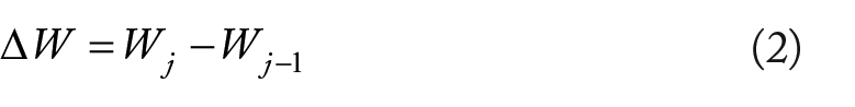
Figure 3 displays the temporal dynamics of daily T_a and its distribution at different P levels. The T_a values per day ranged from 17.15 to 35.28°C, with the average value of 28.04°C, which showed a trend of first rising and then falling. The box diagrams of daily T_a at different P levels had a decrease trend from P1 to P5, with a perfectly (R² = 0.99) and significantly (p < .01) binomial fitting for the average T_a. So daily T_a was negatively correlated with daily P, with the average values of 29.23, 27.70, 25.86, 24.13, and 21.25°C from P1 to P5 levels, respectively. Meanwhile, the daily T_a showed a normal distribution. 27.6 ± 1.5°C appeared most frequently (32 days), accounting for 34.41% of the total time. The highest T_a only occurred in 1 day, and the lowest T_a was found in 4 days.

Figure 3.

Temporal dynamics of daily T_a and its distribution at different P levels.

Temporal dynamics of W at the daily, weekly, and monthly scales

The temporal dynamics of soil water storage (W) response to P and T_a at different scales are shown in Figure 4. At the daily scale, the W in different treatments always had a positively and similarly change trend with daily P but negative trend with daily T_a, and the W peaks delayed 0–2 days after each daily P peak (Figure 4A). The NC treatment showed the lowest values of daily W in most time, with a rapid declination after ending rainfall processes, which ranged from 15.1 to 50.0 mm with the average value of 22.5 mm. The CR treatment tended to have the medium daily W, but owned the highest W peaks after rainfall peaks, exhibiting a similarly and more slightly downward trend with NC treatment. The daily W in the CR treatment ranged from 21.6 to 57.2 mm with the average value of 29.0 mm. The OR treatment showed the highest values of daily W in most time. However, in the last rainfall processes (September 8–11), both of daily W peaks in NC and CR treatments were higher than that in OR treatment. The daily W of OR showed a relatively stable trend over time, with an average value of 31.4 mm, ranging from 26.3 to 51.1 mm.

Figure 4.

Dynamics of W with P and T_a at the daily (A), weekly (B), and monthly (C) scales.

At the weekly scale, the W in the NC, CR, and OR treatments ranged 16.8–42.8 mm, 23.3–49.7 mm, and 28.1–47.3 mm, respectively (Figure 4B). The change trends of weekly W in different treatments were similar to those at the daily scale, which also had a delay effect, and CR treatment had the highest weekly W only in the 3th, 14th, and 15th weeks. In the 3th week, the weekly W in the three treatments were all higher than the 2th and 4th weeks, with the lowest weekly P and Ta among the three weeks. In the 14th week, it showed the highest weekly P and lowest weekly Ta among all weeks. However, in the 15th week, the weekly P was very little, and the weekly W in the OR treatment was found to instead increase. Besides, in the 5th and 7th weeks, the weekly P was zero with the highest weekly Ta of over 31°C, but the weekly W was not the lowest.

At the monthly scale, the W in the NC, CR, and OR treatments ranged 19.2–34.2 mm, 25.7–40.9 mm and 28.9–40.6 mm, respectively (Figure 4C). The change trends of monthly W in different treatments were also OR > CR > NC, except for September with CR > OR. However, the W of August was lower than that of June, whose monthly P (38.8 mm) was far higher than the latter (22.8 mm). It indicated that the trends of monthly W over time were not fully synchronized with monthly P, but remained a completely negative synergistic relationship with monthly T_a.

Relationships of W and ∆W with P and T_a at different time scales

The linear fitting relationships between soil water (W and ∆W) and climatic factors (P and T_a) are shown in Figures 5 to 7. At the daily scale (Figure 5), P was positively and T_a was negatively correlated with W and ∆W, respectively. Daily P had little correlation with daily W (R² = 0.01–0.04) due to the huge disturbance of no-rain days (P1 level in Figure 2), while daily T_a could explain about 23 to 25% of the variation in daily W. However, daily P played an important role in the daily ∆W variation, accounting for 53 to 63% of the contribution, and the contribution of daily T_a still remained lower level of about 17 to 21%. When daily P increased 1.0 mm or daily T_a increased 1.0°C, daily ∆W would increase 0.30 to 0.58 mm or decrease 0.12 to 0.25 mm, respectively. Thus, P had more contribution and influence than T_a in controlling ∆W at the daily scale. Besides, the responses of daily ∆W to the change of P and T_a were the lowest in the OR treatment, and were near to the same in NC and CR treatments.

Figure 5.

Relationships of W and ∆W versus P and T_a at the daily scale.

Figure 6.

Relationships of W and ∆W versus P and T_a at the weekly scale.

Figure 7.

Relationships of W and ∆W vs. P and T_a at the monthly scale.

At the weekly scale (Figure 6), the explanatory power of P to W and ∆W increased to 7 to 12% and decreased to 34 to 37%, respectively. However, the contribution of weekly T_a to the variation in weekly W and ∆W had a huge boost, which were 72 to 77% and 73 to 80%, respectively. When weekly P increased 1.0 mm or weekly T_a increased 1.0°C, the weekly ∆W had a lower increase of 0.24 to 0.38 mm or had a larger decrease of 1.0 to 1.5 mm, respectively. As a result, T_a became more effective than P in controlling ∆W at the weekly scale. Besides, the changes of weekly ∆W relative to P and T_a were still the lowest in the OR treatment, and the fitting lines of NC and CR were also close to coincide.

At the monthly scale (Figure 7), P and T_a had the similar explanatory power of 70 ± 4% to the W variation. The contribution of monthly P and T_a to monthly ∆W variation both increased, which reached 77 to 81% and 93 to 95%, respectively. Monthly P and T_a showed more importance to monthly ∆W than that at the weekly scale. The monthly ∆W would increase 0.36 to 0.48 mm when monthly P increased 1.0 mm, or decrease 2.0 to 2.6 mm when monthly T_a increased 1.0°C. The differences between fitting lines of NC and CR treatments became larger. The lowest responses of monthly ∆W to P and T_a were still shown in the OR treatment, but the largest occurred in the CR treatment.

Correlation between W, P, and T_a

Partial correlation analysis is used to study the effect of T_a on the correlation between P and W (Table 1). Without the effect of T_a, P was found a significantly correlation with W at daily, weekly and monthly scales, and the correlation coefficients (r-values) were 0.20, 0.50 and 0.74, respectively. However, the correlation became insignificant (p > .05) with the controlling variable of T_a, demonstrating the important role of T_a in the P–W relationship. Moreover, the significant levels (p-values) showed a trend of weekly (0.71) > daily (0.21) > monthly (0.21), indicating that T_a might have the largest effect on the relationship of P and W at the weekly scale.

Table 1.

Partial Correlation Analysis Between P and W Controlled by T_a at Different Time Scales.

Controlling variable	Statistics	P
Controlling variable	Statistics	Daily	Weekly	Monthly
None	r-Value	.199	.500	.736
None	p-Value	.001	.001	.024
T_a	r-Value	.075	−.063	–.500
T_a	p-Value	.214	.708	.207

Note. r-Value was the correlation coefficient, and p-value was the value of significant level.

Thresholds of P and T_a to increase soil water

Table 2 displays the thresholds of the lowest P and the highest T_a to increase soil water based on the fitting curves in Figures 5 to 7. Only when the P values were higher and the T_a values were lower than the corresponding thresholds at different time scales, the ∆W could exceed zero value, resulting of the increase of W. The P thresholds had the mean values of 0.93, 4.98, and 28.17 mm at the daily, weekly and monthly scales, respectively. The OR treatment had the lowest P thresholds of 0.80 and 4.13 mm at daily and weekly scales, respectively, but the highest threshold of 28.56 mm at the monthly scale. The NC treatment showed the opposite trend to OR treatment, where CR always owned the medium thresholds with the time scale change. The T_a thresholds also increased with the expanded scale, with the mean values of 28.69, 28.89, and 29.36°C at the daily, weekly and monthly scales, respectively. The OR treatment showed the lowest T_a thresholds at daily and monthly scales, but the highest at the weekly scale. The NC treatment showed the opposite trend of T_a thresholds at daily and monthly scale, but showed the medium value at the weekly scale.

Table 2.

The Thresholds of the Lowest P and The Highest T_a to Increase Soil Water (∆W > 0).

	The lowest P threshold			The highest T_a threshold
	Daily	Weekly	Monthly	Daily	Weekly	Monthly
NC	1.00	5.42	27.61	29.50	28.86	29.50
CR	1.00	5.39	28.35	28.56	28.83	29.29
OR	0.80	4.13	28.56	28.00	28.99	29.29
Mean value	0.93	4.98	28.17	28.69	28.89	29.36

Effects of different treatments on rainwater retention and loss rates

Figure 8 shows the cumulative total amount of P, ∆W, infiltration, and loss during the study period, and calculates the rainwater retention rate and loss rate. The total P amount of the three treatments was the same of 136 mm. The NC treatment had the largest ∆W amount (20.8 mm) and rainwater retention rate (15.29%), followed by the CR treatment with ∆W amount of 19.5 mm and retention rate of 14.34%, and the OR treatment owned the lowest ∆W amount (15.7 mm) and retention rate (11.54%) (Figure 8A). The total infiltration also had a trend of NC (74.75 mm) > CR (72.00 mm) > OR (41.25 mm), and the total loss amount was also ordered by NC (53.95 mm) >CR (52.50 mm) > OR (25.55 mm). However, the trend of soil water loss rate changed to CR (72.92%) > NC (72.17%) > OR (61.94%) (Figure 8B). The results indicated that the OR treatment was difficult to conduct both processes of rainfall-infiltration and infiltration-loss, which had the highest capacity to conserve existing soil water.

Figure 8.

Cumulative ∆W amount and the rainwater retention rate (A), and cumulative infiltration, loss and loss rate of soil water (B). Rainwater retention rate was the ratio of cumulative ∆W amount to total P amount. Total infiltration was the cumulative amount of positive ∆W per day. Total loss was the cumulative amount of negative ∆W per day. Loss rate was the ratio of total loss to total infiltration.

Discussion

Synergic relationship between P and T_a

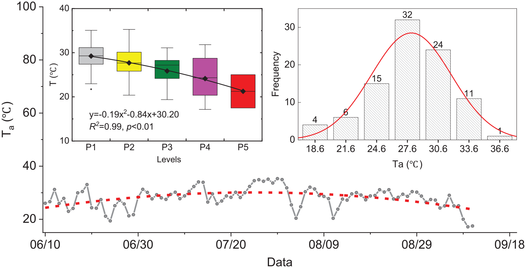
Precipitation (P) and air temperature (T_a) were the main factors to reflect climate change (Hurrell, 1995), which were important to soil hydrological processes. More P amount brought higher replenishment of soil water, and higher T_a would produce more evapotranspiration resulting in more loss of soil water. We found that most frequency (more than 90%) of rainy days had a little of daily P amount ⩽ 5 mm, accounting for less than 30% of total P amount, while more than 70% of total P amount occurred only in less than 10% of rainy days (Figure 2). The average T_a of different P levels gradually decreased from P1 to P5, which verified the negatively synergic relationship between P and T_a (Figure 9). It indicated that each increase of 1.0 mm of P would cause a decrease of about 0.5°C of T_a. Daily P only explained 16% of variation in daily T_a, but the explanatory power increased to 95% for P1 to P5 levels. So, the synergic relationship between P and T_a might produce large effects on soil water. The results of partial correlation (Table 1) also verified this assumption that the effect of P on W was controlled by T_a during the observation period. The effectiveness of P on soil water supplementation depended on the amount of loss affected by T_a. Studying the change of soil water should consider both the role of P and T_a.

Figure 9.

The relationships between P and T_a for P1 to P5 levels (A) and every day (B).

Dynamics of soil water response to P and T_a

The W represented the status of soil water conservation, controlled by P and T_a (Agboma and Itenfisu, 2020). In this study, we found soil water positively responded to P and negatively responded to T_a (Figures 4 to 7). Daily P showed little contribution (1–4%) to the variation of daily W, while daily T_a showed approximate 23 to 25% of contribution to daily W variation. As for the ∆W of every day, it was strongly controlled by daily P (53–63% of contribution) but weakly affected by daily T_a (17–21% of contribution). Thus, at the daily scale, P was the main factor to affect the ∆W, and T_a was more responsible for the status of W during the observation period. The reasons might be that the W of a certain day was often largely influenced by its early status before rainfall events (Dai and Wang, 2021). For example, a low amount of daily P possibly happened in the days with the high W, and a high amount of daily P happened in the days with the low W. Besides, the high proportion of no-rain days (Figure 2) and the delayed effect of P on W (Figure 4) also disturbed the P-W relationship at the daily scale. Moreover, P always could replenish soil water through rainfall infiltration processes, which would bring rapid responses and differences of ∆W at daily scale (Liu et al., 2023).

On the other hand, the loss of soil water induced by soil water evaporation from high T_a was a slow process, more ET happened after rainfall events over time, resulting in a continued long-term effect of T_a on W through the ET processes on each day (Fang et al., 2019; Longobardi and Khaertdinova, 2015). So, the contribution of T_a to soil water at short time scale was lower, and the weak and sustained long-term cumulative effect greatly enhanced the function of T_a in soil water at longer time scale. The high contributions of T_a to soil water at the weekly scale (72–80%) and at the monthly scale (66–95%) (Figures 6–7) also confirmed the above opinion and the cumulative effect on soil water loss. Previous studies also proved the importance of T_a in soil water with negative effects (Fang et al., 2019; Shih, 2022; Xiang et al., 2013), and the explanatory contribution could reach 60 to 80% as well (Shih et al., 1991).

According to the results of Figures 5 to 7, we found that the contribution of P and T_a to soil water was varied from daily, weekly to monthly time scales. P had more influence to ∆W than T_a at the daily scale, while the contribution of P to ∆W decreased to 34 to 37% at the weekly scale but increased to 67 to 81% at the monthly scale, which were both lower than those of T_a. Therefore, P played a key role in the daily ∆W, determining the amount of soil water replenishment, but the retention amount of soil water depended on the ET loss controlled by T_a (Ramos and Martinez-Casasnovas, 2010). The soil water conservation was the combined effect of P and T_a (Jin et al., 2018; Longobardi and Khaertdinova, 2015; Ni et al., 2019), with different mechanisms at different time scales.

Threshold analysis on soil water conservation

For some days with low daily P and high daily T_a, the water storage instead decreased (∆W < 0) on rainy days. The threshold effect of P and T_a on soil water has been proven by previous studies (Dai and Wang, 2021; Ge et al., 2022; Jin et al., 2018; Liu et al., 2023). 5 to 14 mm of rainfall events was required to trigger soil water increase at 10 cm soil depth in grassland and forestland (Ge et al., 2022; Jin et al., 2018). Rainfall amount >7.0 mm could effectively offset the water consumption from processes of ET, vegetation interception and other losses (Dai and Wang, 2021; Liu et al., 2018; Ni et al., 2019). Furthermore, rainfall amount more than 30 mm promoted rainfall water infiltrate more than 60 cm soil depth in planted forest (Chen et al., 2020). In this study, we also revealed the threshold phenomena of P and T_a at different time scales. At the daily scale, P should be larger than 0.93 mm and T_a should be lower than 28.69°C to increase soil water for grassland. At the weekly scale, the thresholds of P and T_a were 4.98 mm and 28.89°C, respectively. At the monthly scale, the thresholds of P and T_a were 28.17 mm and 29.6°C, respectively (Table 2). The increase order of thresholds over time verified the tolerance of soil water changes to climatic conditions over time. Base on the fitting equations in Figures 5 to 7, we could simulate the super-extreme drought scenario that soil dried without any soil water in grassland, which required daily T_a over 64.46°C, or weekly T_a over 41.4°C, or monthly T_a over 39.22°C. This simulated scenario also proved the cumulative effects and tolerance of soil water loss over time, and provided a reference for dealing with future extreme conditions and climate change.

Effects of grass components on soil water retention and loss

Different plant components have been proven to significantly affect soil water (Liu et al., 2023). In this study, we found that soil water storage had a trend of OR > CR > NC. This result is agreed with the knowledge that the roots promote rainwater infiltration and the canopy consume soil water (Fang et al., 2019; Wang et al., 2022b). There is a common understanding that the canopy intercepted rainfall and increased transpiration, leading to a negative effect on soil water replenishment (Fang et al., 2019; Liu et al., 2018; Wang et al., 2022a). The roots could form horizontal and vertical underground networks to promote water transport, and also improve soil physical and chemical properties to enhance infiltration capacity (Cui et al., 2019; Luo et al., 2022; Wu et al., 2017). However, the lowest soil water storage in the NC treatment indicated the negative effect of the litter cover on conserving soil water, which was opposite to previous opinions that the litter could prevent evaporation, delay the generation of runoff, and decompose organic matter to improve soil properties, leading to increase the infiltration capacity (Cui et al., 2021; Xiong et al., 2008; Zhao et al., 2022). This could be explained that the interception of rainfall by the litter decreased the input of soil water for small rainfall events (Zhao et al., 2022), and the promotion of runoff due to the cover path from litter by litter (Liu et al., 2018).

In addition, soil hydrological processes differed from the three treatment types with different grass components. The replenishment of soil water mainly occurred in September during the growing season (Figure 4C), leading to a positively cumulative ∆W for all treatments (Figure 8A). We found the cumulative ∆W and the rainwater retention rate had the same trend of NC > CR > OR, as well as the trends of total infiltration and total loss (Figure 8). The results indicated that the grass canopy promoted the total input and output of soil water, the grass litter played a role in preventing soil water loss, and the grass roots had more effects on holding soil water due to the lowest loss rate of soil water. It could be explained that the grass canopy was close to soil, and coupling with the interception function of the litter, the aboveground and surface cover of grass stored more rainfall and runoff, which became the source of water infiltration. In general, the grassland if only roots had the lowest total infiltration, but the lowest loss rate also supported that the roots had significant effects on conserving soil water after infiltration processes.

The effects of P and T_a on soil water were significantly influenced by grass components. The fitting lines of ∆W with P and T_a were similar and close to coincide between the NC and CR treatments across the time scales, indicating that the grass litter had few effects on triggering the increase or decrease of soil water by P and T_a. The slope values of fitting lines in the OR treatment were always lower than other treatments, leading to the lowest relative increase of soil water to increase P or decrease T_a, which illustrated that the response of soil water to climate change was strengthened by the grass canopy and weakened by the roots, which had different performances in shrubland (Liu et al., 2023). The last stage of the growing season was the most effective time to increase soil water reserves, which reduced water consumption due to the weak transpiration and water evaporation activity, especially with large rainfall events. So, canopy and litter cover in grassland is crucial to conserve soil water. The change of vegetation structure and function and its response to climate change (e.g. P and T_a) under the drought stress need more attention (Yu et al., 2023).

Conclusions

Precipitation (P) and air temperature (T_a) both affected surface soil water significantly. However, these effects were influenced by grass components and time scales. In this study, we found a negatively synergistic relationship between P and T_a, especially to analyze the change under different levels of P amount. The surface soil water changed positively with P and negatively with T_a at different time scales, and had a trend of OR > CR > NC for most time. However, the responses of ∆W to P and T_a varied with different time scales and grass component treatments. At the daily scale, P had more contribution (53–63%) to ∆W than that of T_a (17–21%). At the weekly scale, T_a became the main explanatory factor (73–80%) to ∆W variation. At the monthly scale, both P and T_a showed high contributions (77–81% and 93–95%, respectively). In most cases, the OR treatment displayed the lowest sensitivity to the change of P and T_a, while the NC and CR treatments had the similar response, indicating that the response of soil water to climate change was strengthened by the grass canopy and weakened by the roots. Besides, the effects of P on surface soil water were largely controlled by the T_a factor. The effect of P and T_a on increasing soil water existed thresholds, which ranged 0.93 to 28.17 mm and 28.69 to 29.36°C from the daily to weekly and to monthly scale. During the whole study period, all of the total infiltration, total loss and rainwater retention rate had the same trend of NC > CR > OR, indicating that grass canopy and litter promote to conserve soil water, and the increasing amount could offset the consumption of soil water. The roots showed a positive function in infiltration and had the lowest soil water loss rate. This study is beneficial to soil water conservation in grassland to face the challenge of climate change in the Loess Plateau.

Footnotes

Declaration of Conflicting Interests

The author(s) declared no potential conflicts of interest with respect to the research, authorship, and/or publication of this article.

Funding

The author(s) disclosed receipt of the following financial support for the research, authorship, and/or publication of this article: This research was supported by the National Natural Science Foundation of China (nos. 42201126, U2243231, 41971037, 42201103, and 42001020), and the Open Foundation of the State Key Laboratory of Urban and Regional Ecology of China (no. SKLURE2020-2-3), and the Scientific Research Plan Project of Tianjin Municipal Education Commission (no. 2019KJ091).

Data Availability

Data will be made available on request.

ORCID iD

Jianbo Liu

References

Agboma

Itenfisu

(2020). Investigating the spatio-temporal dynamics in the soil water storage in alberta’s agricultural region. Journal of Hydrology, 588, 125104. https://doi.org/10.1016/j.jhydrol.2020.125104

Allen

S. T.

Brooks

J. R.

Keim

R. F.

Bond

B. J.

McDonnell

J. J.

(2014). The role of pre- event canopy storage in throughfall and stemflow by using isotopic tracers. Ecohydrology, 7(2), 858–868. https://doi.org/10.1002/Eco.1408

Chen

W. L.

Z. S.

Jiao

Wang

Gao

G. Y.

B. J.

(2020). Response of soil moisture to rainfall event in black locust plantations at different stages of restoration in hilly-gully area of the Loess Plateau, China. Chinese Geographical Science, 30(3), 427–445. https://doi.org/10.1007/s11769-020-1121-4

Cui

Huang

Luo

Qiu

K. Y.

Lopez-Vicente

G. L.

(2021). Litter cover breaks soil water repellency of biocrusts, enhancing initial soil water infiltration and content in a semi-arid sandy land. Agricultural Water Management, 255, 107009. https://doi.org/10.1016/j.agwat.2021.107009

Cui

G. L.

Huang

Liu

(2019). Fine roots determine soil infiltration potential than soil water content in semi-arid grassland soils. Journal of Hydrology, 578, 124023. https://doi.org/10.1016/j.jhydrol.2019.124023

Dai

Wang

(2021). Influence of rainfall events on soil moisture in a typical steppe of Xilingol. Physics and Chemistry of the Earth, 121, 102964. https://doi.org/10.1016/j.pce.2020.102964

Jiao

Yao

Fang

(2019). Effects of precipitation changes on soil moisture characteristics of returning farmland in loess hilly region. Research of Soil and Water Conservation, 26(5), 81–88.

Fang

W. W.

Liu

J. B.

Jiao

Zhang

Wang

M. Y.

B. J.

(2019). Canopy transpiration and stand water balance between two contrasting hydrological years in three typical shrub communities on the semiarid Loess Plateau of China. Ecohydrology, 12(2), e2064. https://doi.org/10.1002/eco.2064

B. J.

Wang

Liu

J. B.

Liang

Miao

C. Y.

(2017). Hydrogeomorphic ecosystem responses to natural and anthropogenic changes in the loess plateau of China. Annual Review of Earth and Planetary Sciences, 45, 223–243. https://doi.org/10.1146/annurev-earth-063016-020552

10.

F. C.

M. X.

Gong

Zhang

Z. Y.

Tan

Q. Y.

Pan

X. H.

(2022). Land cover changes the soil moisture response to rainfall on the Loess Plateau. Hydrol Process, 36(11), 14714. https://doi.org/10.1002/hyp.14714

11.

Good

S. P.

Noone

Bowen

(2015). Hydrologic connectivity constrains partitioning of global terrestrial water fluxes. Science, 349(6244), 175–177. https://doi.org/10.1126/science.aaa5931

12.

Han

Y. P.

Xia

Huang

H. P.

W. B.

Jia

D. D.

(2022). Impact of the grain for green project on water resources and ecological water stress in the Yanhe River Basin. Plos One, 17(6), e0259611. https://doi.org/10.1371/journal.pone.0259611

13.

Z. M.

Jia

G. D.

Liu

Z. Q.

Zhang

Z. Y.

X. X.

Hao

P. Q.

(2020). Field studies on the influence of rainfall intensity, vegetation cover and slope length on soil moisture infiltration on typical watersheds of the Loess Plateau, China. Hydrological Processes, 34(25), 4904–4919. https://doi.org/10.1002/hyp.13892

14.

Hurrell

J. W.

(1995). Decadal trends in the North-Atlantic oscillation–regional temperatures and precipitation. Science, 269(5224), 676–679. https://doi.org/10.1126/science.269.5224.676

15.

Jiao

B. J.

Gao

G. Y.

Wang

Jin

T. T.

Zhang

L. W.

Liu

J. B.

Zhang

(2016). Comparison of transpiration between different aged black locust (Robinia pseudoacacia) trees on the semi-arid Loess Plateau, China. Journal of Arid Land, 8(4), 604–617. https://doi.org/10.1007/s40333-016-0047-2

16.

Jin

Guo

Lin

Wang

Y. Q.

Y. L.

Chu

G. C.

Zhang

(2018). Soil moisture response to rainfall on the Chinese Loess Plateau after a long-term vegetation rehabilitation. Hydrological Processes, 32(12), 1738–1754. https://doi.org/10.1002/hyp.13143

17.

Liu

J. B.

Gao

G. Y.

Wang

Jiao

B. J.

(2018). The effects of vegetation on runoff and soil loss: Multidimensional structure analysis and scale characteristics. Journal of Geographical Sciences, 28(1), 59–78. https://doi.org/10.1007/s11442-018-1459-z

18.

Liu

J. B.

Liang

Gao

G. Y.

Dunkerley

B. J.

(2022). Quantifying the effects of rainfall intensity fluctuation on runoff and soil loss: From indicators to models. Journal of Hydrology, 607, 127494. https://doi.org/10.1016/j.jhydrol.2022.127494

19.

Liu

Gao

Zhang

(2023). Effect of shrub components on soil water and its response to precipitation at different time scales in the loess plateau. International Journal of Environmental Research and Public Health, 20(6), 4722. https://doi.org/10.3390/ijerph20064722

20.

Liu

X. M.

Zhang

(2013). Trend analysis of reference evapotranspiration in Northwest China: The roles of changing wind speed and surface air temperature. Hydrological Processes, 27(26), 3941–3948. https://doi.org/10.1002/hyp.9527

21.

Liu

Y. J.

Yang

J. M.

Tang

C. J.

Zheng

H. J.

(2016). Characteristics of the surface-subsurface flow generation and sediment yield to the rainfall regime and land-cover by long-term in-situ observation in the red soil region, Southern China. Journal of Hydrology, 539, 457–467. https://doi.org/10.1016/j.jhydrol.2016.05.058

22.

Longobardi

Khaertdinova

(2015). Relating soil moisture and air temperature to evapotranspiration fluxes during inter-storm periods at a Mediterranean experimental site. Journal of Arid Land, 7(1), 27–36. https://doi.org/10.1007/s40333-014-0075-8

23.

Luo

Z. T.

Niu

J. Z.

S. Q.

Zhang

Chen

X. W.

Tan

Wang

Berndtsson

(2022). Linking roots, preferential flow, and soil moisture redistribution in deciduous and coniferous forest soils. Journal of Soils and Sediments, 23, 1524–1538. https://doi.org/10.1007/s11368-022-03375-w

24.

J. J.

Cheng

Y. F.

Wang

Q. H.

C. W. W.

Garg

(2019). Effects of vegetation on soil temperature and water content: Field monitoring and numerical modelling. Journal of Hydrology, 571, 494–502. https://doi.org/10.1016/j.jhydrol.2019.02.009

25.

Qiu

D. X.

R. R.

C. X.

X. M.

Zhao

G. J.

Gao

(2023). Effects of vegetation restoration on soil infiltrability and preferential flow in hilly gully areas of the Loess Plateau, China. Catena, 221, 106770. https://doi.org/10.1016/j.catena.2022.106770

26.

Ramos

M. C.

Jones

G. V.

Martinez-Casasnovas

J. A.

(2008). Structure and trends in climate parameters affecting winegrape production in northeast Spain. Climate Research, 38(1), 1–15. https://doi.org/10.3354/cr00759

27.

Ramos

M. C.

Martinez-Casasnovas

J. A.

(2010). Effects of precipitation patterns and temperature trends on soil water available for vineyards in a Mediterranean climate area. Agricultural Water Management, 97(10), 1495–1505. https://doi.org/10.1016/j.agwat.2010.05.003

28.

Shih

D. C. F.

(2022). Coherence between sunlight quantum and soil water content in the shallow quaternary gravel layer: Evidence of the spectral analysis. Journal of Hydrology, 608, 127578. https://doi.org/10.1016/j.jhydrol.2022.127578

29.

Shih

S. F.

Harrison

D. S.

Smajstrla

A. G.

Zazueta

F. S.

(1991). Infrared thermometry to estimate soil-water content in pasture areas. Soil and Crop Science Society of Florida, 50, 158–162.

30.

Tanaka

Hashimoto

(2006). Plant canopy effects on soil thermal and hydrological properties and soil respiration. Ecological Modelling, 196(1–2), 32–44. https://doi.org/10.1016/j.ecolmodel.2006.01.004

31.

Wang

Zhang

(2022a). Measurement and modeling of canopy interception losses by two differently aged apple orchards in a subhumid region of the Yellow River Basin. Agricultural Water Management, 269, 107667. https://doi.org/10.1016/j.agwat.2022.107667

32.

Wang

H. F.

Zhu

X. A.

Zakari

Chen

C. F.

Liu

W. J.

Jiang

X. J.

(2022b). Assessing the effects of plant roots on soil water infiltration using dyes and hydrus-1D. Forests, 13(7), 1095. https://doi.org/10.3390/f13071095

33.

Wang

Gao

Liu

Zhou

(2013). Responses of soil moisture in different land cover types to rainfall events in a re-vegetation catchment area of the Loess Plateau, China. Catena, 101, 122–128. https://doi.org/10.1016/j.catena.2012.10.006

34.

Wang

Y. Q.

Shao

M. A.

Zhu

Y. J.

Liu

Z. P.

(2011). Impacts of land use and plant characteristics on dried soil layers in different climatic regions on the Loess Plateau of China. Agricultural and Forest Meteorology, 151(4), 437–448. https://doi.org/10.1016/j.agrformet.2010.11.016

35.

G. L.

Liu

Yang

Cui

Deng

Chang

X. F.

Shi

Z. H.

(2017). Root channels to indicate the increase in soil matrix water infiltration capacity of arid reclaimed mine soils. Journal of Hydrology, 546, 133–139. https://doi.org/10.1016/j.jhydrol.2016.12.047

36.

Xiang

X. H.

X. L.

Wang

C. H.

Chen

Shao

Q. Q.

(2013). Influences of climate variation on thawing-freezing processes in the northeast of three-river source region China. Cold Regions Science and Technology, 86, 86–97. https://doi.org/10.1016/j.coldregions.2012.10.006

37.

Xiong

Y. M.

Xia

H. X.

Z. A.

Cai

X. A.

S. L.

(2008). Impacts of litter and understory removal on soil properties in a subtropical Acacia mangium plantation in China. Plant Soil, 304(1–2), 179–188. https://doi.org/10.1007/s11104-007-9536-6

38.

Hua

Chen

Zhang

Pereira

(2023). Divergent changes in vegetation greenness, productivity, and rainfall use efficiency are characteristic of ecological restoration towards high-quality development in the Yellow River Basin, China. Engineering. Advance online publication. https://doi.org/10.1016/j.eng.2023.07.012

39.

Zhao

W. W.

Martinez-Murillo

J. F.

Pereira

(2020). Loess plateau: From degradation to restoration. Science of the Total Environment, 738, 140206. https://doi.org/10.1016/j.scitotenv.2020.140206

40.

Zhu

R. P.

D. M.

Liu

D. J.

Liu

Gao

Z. Q.

Yin

M. Q.

Bandala

E. R.

Rodrigo-Comino

(2022). Multiple surface runoff and soil loss responses by sandstone morphologies to land-use and precipitation regimes changes in the Loess Plateau, China. Catena, 217, 106477. https://doi.org/10.1016/j.catena.2022.106477

41.

Zhang

D. H.

X. R.

Zhang

Z. S.

Chen

Y. L.

(2016). Effects of rainfall intensity and intermittency on woody vegetation cover and deep soil moisture in dryland ecosystems. Journal of Hydrology, 543, 270–282. https://doi.org/10.1016/j.jhydrol.2016.10.003

42.

Zhao

L. S.

Meng

Zhang

J. S.

Zhang

J. X.

Sun

S. J.

C. X.

(2022). Effect of slopes on rainfall interception by leaf litter under simulated rainfall conditions. Hydrological Processes, 36(8), e14659. https://doi.org/10.1002/hyp.14659

Effect of Grass Components on the Temporal Response of Surface Soil Water to Precipitation and Air Temperature in the Loess Plateau

Abstract

Keywords

Introduction

Materials and Methods

Study area

Field experiments

Data analysis

Results

The characteristics of P and Ta per day during the study period

Temporal dynamics of W at the daily, weekly, and monthly scales

Relationships of W and ∆W with P and Ta at different time scales

Correlation between W, P, and Ta

Thresholds of P and Ta to increase soil water

Effects of different treatments on rainwater retention and loss rates

Discussion

Synergic relationship between P and Ta

Dynamics of soil water response to P and Ta

Threshold analysis on soil water conservation

Effects of grass components on soil water retention and loss

Conclusions

Footnotes

Declaration of Conflicting Interests

Funding

Data Availability

ORCID iD

References

The characteristics of P and T_a per day during the study period

Relationships of W and ∆W with P and T_a at different time scales

Correlation between W, P, and T_a

Thresholds of P and T_a to increase soil water

Synergic relationship between P and T_a

Dynamics of soil water response to P and T_a