Sage Journals: Discover world-class research

Abstract

Noncoding RNAs (ncRNAs) play significant roles in multiple fundamental biological processes, in particular, ncRNAs interactions provide valuable insights into protein synthesis, controlling gene expression, RNA processing, regulation of localization, etc. The dysregulation of ncRNA interaction may cause severe diseases including cancer. Therefore, developing computational methods for investigating ncRNA-protein interaction has become a problem of interest for researchers. In this study, we proposed a novel deep learning (DL) model named RPI-SDA-XGBoost for predicting the interaction between ncRNA and proteins. We utilized the 3-mer conjoint triad feature (CTF) to encode the protein sequence, and the 4-mer frequency to encode the RNA sequence, resulting in the extraction of a total of 599-dimensional vector features. The DL approach is developed based on stack denoising autoencoder (SDA) to discover high-level hidden characteristics from 2 separate networks representing proteins and ncRNAs. Composition of features were fed into XGBoost based meta-learner for the final prediction. Proposed model, RPI-SDA-XGBoost, outperformed most of the individual baseline models and significantly improved the performance on multiple benchmark data sets. We validate the generalization power of the proposed model on five benchmark data sets, namely, RPI_ 369, RP_I488, RPI_1807, RPI_ 2241, and NPInterv2.0. RPI-SDA-XGBoost achieved similar levels of state-of-the-art accuracy on data sets RPI_488, RPI_1807, and RPI_NPInter v2.0. Proposed model achieved the best precision of 87.9% and 94.6% in the largest two data sets RPI_ 2241, and RPI_NPInter v2.0, respectively. We believe the proposed model provides useful direction for upcoming biological research and suggesting more sophisticated computational approaches are warranted in near future for ncRNA protein interaction predictions.

Keywords

Noncoding RNAs (ncRNAs)stacked auto-encoders (SAE)stacked denoising autoencoder (SDA)extreme gradient boosting (XGBoost)conjoint triad feature (CTF)

Introduction

Noncoding RNAs (ncRNAs) are a sub-family of RNAs, constituting approximately 98% of all RNA transcribed from the human genome that is not converted into proteins.¹ Since it was shown that only around 2 % of the human genome is composed of sequences that encode proteins, with the balance being noncoding regions, we have come to see the transcriptional landscape in eukaryotic creatures like humans as being significantly more complex than previously believed. The majority of the human genome is ubiquitously transcribed into noncoding RNAs (ncRNAs), regardless of whether it encodes a protein.² Researchers have discovered thousands of new ncRNAs, including miRNAs, siRNAs, snoRNAs, piRNAs, and lncRNAs, and many of their functions remain still unclear. According to GENCODE v23, which came out in 2015, the human genome has about 60 000 genes. Only 20 000 of them are protein-coding genes, whereas over 40 000 are ncRNA genes.³ The number of ncRNAs is growing every year.⁴ In addition, many researchers find it quite confounding that each ncRNA plays a unique function in the processes of protein translation. Recent studies indicate that the imbalance of noncoding RNAs is associated with the development of various serious diseases.^5,6

Furthermore, an increasing body of evidence from recent studies confirms that the disequilibrium of ncRNAs, which are essential for several biological processes, such as the control of posttranscriptional genes, is linked to the occurrence of a series of major diseases.⁷ In the meanwhile, various cutting-edge technologies have found more and more ncRNAs with unknown roles.^1,8,9 Thus, it is critical to clearly characterize the biological roles of these ncRNAs, including RNA translation and stability.

For example, as a case study, interactions between the oncogenic lncRNA MALAT1 and RNA-binding proteins (RBPs) can be discussed through multiple non-AI methodologies, such as each (a) Yeast Two-Hybrid (Y2H), (b) Cross-linking immunoprecipitation sequencing (CLIP-seq), (c) Molecular Docking Simulation (MDS), (d) Motif analysis. Y2H systems remain the gold standard for validating direct protein-RNA interactions due to their high specificity and low false positive rate in detecting binary molecular interactions. But, this method is severely limited by its low-throughput nature and inability to capture indirect or weak interactions that may be biologically significant. For more comprehensive in vivo analysis, CLIP-seq techniques (such as HITS-CLIP, PAR-CLIP, or iCLIP) provide nucleotide-resolution mapping of protein-RNA binding sites across the entire transcriptome. But CLIP-based methods require expensive instrumentation, specific antibodies for each RBP of interest, and complex bioinformatics pipelines for data analysis.

Molecular docking simulations (MDS) offer valuable structural insights by computationally predicting 3-dimensional binding conformations and interaction between RNA and proteins. But it requires high-performance computing resources and accurate structural models of both the RNA (often lacking for lncRNAs like MALAT1) and protein/ligand counterpart. At the most accessible end of the computational spectrum, motif-based analyses can rapidly scan sequences for known RBP binding motifs (ie, tools like MEME or HOMER), but these methods frequently miss novel or context-dependent interactions and suffer from high false positive rates due to the degenerate nature of RNA-protein recognition sequences.

Considering the above backdrop of MALAT as a case study, many researchers have proposed several ML techniques to predict ncRNA-binding residues in proteins, including Support Vector Machine (SVM), Random Forest (RF) for RPI-Seq¹⁰ and RPIPred¹¹ and DL techniques such as RPITER, IPMiner, BGFT, and RPI-SAN.^1,3,7,12 Table 1 and Table 2 summarize the tools using ML and DL-based models, respectively.

Table 1.

High-level overview of ML-based ncRNA-protein interaction prediction tools (RPI-Seq, RPI-Pred).

Method used	RPISeq¹⁰	RPI-Pred¹¹
Publication Year	2011	2015
Authors	Muppirala et al	Suresh et al
Benchmark Datasets used and Reference	RPI_369, RPI_2241¹¹	RPI_369, RPI_2241,¹¹ RPI_1807¹³
Type of ncRNA and Protein used	Primary sequence information	High-order 3D structural sequence information and primary sequence
Feature extraction used	Protein: k-mer = 3 (CTFS), RNA: k-mer = 4	Protein (seq., struct.): 7-letter reduced × 16-letter structural fragments = 112 possible combination RNA (seq., struct.): 4(for nucleotide) × 5 (for 3D structures) = 20
Total number of features	343 + 256 = 599 feature vectors	112 + 20 = 132 feature vectors
Model Used	SVM, RF	SVM
Source of Datasets	PRIDB or PDB https://github.com/Pengeace/RPITER	PRIDB or PDB and NPInterv2.0 https://github.com/Pengeace/RPITER
Python code/Implementation)	N/A	http://ctsb.is.wfubmc.edu/projects/rpi-pred

Table 2.

High-level overview of DL-based ncRNA-protein interaction prediction tools (IPMiner, BGFE, RPI-SAN, RPITER).

Method used	IPMiner³	BGFE¹
Publication Year	2016	2019
Authors	Pan et al	Zhan et al
Benchmark Datasets used and Reference	RPI_369, RPI_2241,¹¹ RPI_488,³ RPI_1807,¹³ RPI_NPInterv2.0,¹⁴ RPI_13254	RPI_488,³ RPI_1807,¹³ RPI_2241¹¹
Type of ncRNA and Protein used	Primary sequence information	Primary sequence information
Feature extraction used	Protein: k-mer = 3(CTFS) RNA: k-mer = 4	Protein: PSSM (bi-gram algorithm). RNA: k-mers sparse matrix (SVD).
Total number of features	343 + 256 = 599 feature vectors	N/A
Model Used	Stacked Denoising Autoencoder (SDA)	Stacked Auto-Encoders (SAE)
Source of Datasets	PRIDB or PDB https://github.com/Pengeace/RPITER	PRIDB or PDB https://github.com/Pengeace/RPITER
Python code/Implementation)	http://www.csbio.sjtu.edu.cn/bioinf/IPMiner or https://github.com/xypan1232/IPMiner.	N/A
Method used	RPI-SAN ¹²	RPITER ⁷
Publication Year	2018	2019
Authors	Yi et al	Penf et al
Benchmark Datasets used and Reference	RPI_2241,¹¹ RPI_488,³ RPI_1807,¹³ RPI_NPInterv2.0¹⁴	RPI_488,³ RPI_1807,¹³ RPI_369, RPI_2241,¹¹ RPI_NPInterv2.0¹⁴
Type of ncRNA and Protein used	Primary sequence information	Information about the Primary sequence and structural sequence
Feature extraction used	Protein: PSSM (PZM) RNA: k-mers sparse matrix (SVD).	Protein: (seq., struct.): Improved k-mer = 1-3(CTFS) RNA (seq., struct.): Improved k-mer = 1-4
Total number of features	240 + 256 = 486 feature vectors	837 + 710 = 1547 feature vectors
Model Used	SDA	SAE and CNN
Source of Datasets	PRIDB or PDB https://github.com/Pengeace/RPITER	PRIDB or PDB https://github.com/Pengeace/RPITER
Python code/Implementation)	N/A	https://github.com/Pengeace/RPITER

In addition, according to Diao et al¹³ a comprehensive review of recent literature studies related to long-noncoding RNA interaction (LPI) with exemplary predictive performance over the past 5 years in conjunction with diverse prediction functions was provided. Peng et al⁷ created a DL model called RPITER that made use of 2 fundamental neural network architectures stacked auto-encoders (SAE) and convolutional neural network (CNN). The authors of this work used the enhanced CTF approach to encode the main sequence and sequence structure information to extract features. The range of k was extended to 1-3 mer frequency instead of the 3-mer frequency for the protein CTF technique and 1-4 mer frequency instead of the 4-mer frequency for RNA when the authors applied the enhanced CTF method for sequence information. Compared with the 599 feature vectors that were previously derived from protein and RNA sequences, this led to the production of 739 feature vectors. In addition, they employed the enhanced CTF technique to encode the RNA and protein’s sequence structural information, extracting 370 feature vectors from the RNA and 438 from the protein, for a total of 808 feature vectors from the RNA and protein structure sequences. They showed that their algorithm improves prediction performance based on 5 benchmark data sets. In addition, in 2021, Huang et al¹⁵ proposed the LGFC-CNN model for predicting LPI utilizing a deep learning approach and several feature types. The authors acknowledged that their approach, which mixes handmade characteristics, structural features, and raw sequence composition information, was regarded as a revolutionary deep learning method. They mined 2 kinds of features using CNN modules and 2 sequence preprocessing techniques. In addition, they compared the predictive power of various combinations of lncRNA and protein characteristics to derive hand-designed features. In addition, they used the structural features that were collected and used the Fourier transform to unify the dimensions. To fully forecast the LPIs, the 4 feature kinds are finally combined. LGFC-CNN outperforms other state-of-the-art techniques on 3 benchmark data sets, achieving 94.14% accuracy on RPI21850, 92.94 % accuracy on RPI7317, and 98.19 % accuracy on RPI1847. The results demonstrate that by integrating structural characteristics, hand-designed features, and raw sequence composition data, our LGFC-CNN can reliably predict the interactions between lncRNA and proteins. The EDLMFC approach was also developed by Wang et al,¹⁶ which predicted ncRPI by combining characteristics from an ensemble deep learning framework on many scales. To get properties of proteins and ncRNA from information of the primary sequence, secondary structure, and tertiary structure, they employed the Conjoint k-mer encoding approach. They then used a multilayer deep learning model to include these different characteristics. This model used a bi-directional long short-term memory network (BLSTM) to identify long-term relationships between the CNN-identified features and a convolutional neural network (CNN) to learn the most significant biological information. With 93.8% accuracy on the RPI1807 data set, 89.7% accuracy on the NPInter v2.0 data set, and 86.1% accuracy on the RPI488 data set, EDLMFC outperforms other state-of-the-art techniques in 5-fold cross-validation. Peng et al¹⁷ developed a dual-net neural architecture DL model to identify potential LPIs. PyFeat and BioTriangle were used by the authors to extract the characteristics of proteins and lncRNAs, respectively. Following dimension reduction, these characteristics are then concatenated as a vector. Finally, using 4 cross-validations, we contrasted LPI-DLDN with 6 cutting-edge LPI prediction techniques: LPI-XGBoost, LPI-HeteSim, LPINRLMF, PLIPCOM, LPI-CNNCP, and Capsule-LPI. The outcomes show how well LPI-DLDN performs in LPI categorization. DeepLPI, a unique technique for forecasting interactions between lncRNAs and protein isoforms, was proposed by Shaw et al.¹⁸ This approach uses expression data to derive topological characteristics after using sequence and structural data to get intrinsic features. The authors used a hybrid architecture that combined a conditional random field with a multimodal deep learning neural network. The restricted availability of known interactions was further addressed by using a multiple instance learning (MIL) technique. Experiments comparing the 2 approaches demonstrated that DeepLPI outperformed the state-of-the-art techniques. It raised the AUPRC by 5.9% and the AUC by 4.7%. These findings suggest that DeepLPI may be a valuable tool for predicting the potential interactions between lncRNA and proteins as well as additional roles that RNAs and proteins may play. Ma et al¹⁹ introduced the BiHo-GNN deep learning framework, which predicts the interaction between lncRNA and proteins using graph neural networks (GNNs) and bipartite graph embedding. In contrast to other methods, BiHo-GNN leverages both homogeneous and heterogeneous network characteristics to get a more profound comprehension of molecular relationships. The model also incorporates a reciprocal optimization process to increase robustness. Experiments on 4 data sets showed that BiHo-GNN performs better than other bipartite graph-based methods. This makes it a useful technique for making accurate guesses on the potential relationships and interactions between lncRNA and proteins. LPICGAE, a deep learning framework for forecasting probable human lncRNA-protein interactions, was suggested by Zhao et al.²⁰ First, the model learns low-dimensional representations from high-dimensional lncRNA and protein properties using a variational graph auto-encoder. The adjacency matrix is then rebuilt using a graph auto-encoder to deduce interactions. The anticipated interaction matrix is improved by LPICGAE by alternating between reducing the loss of these processes. With an accuracy of 0.985 and an average AUC of 0.974, the results of the 5-fold cross-validation test demonstrate that LPICGAE outperforms 6 industry-leading techniques. This method offers a potentially useful tool for identifying new lncRNA-protein interactions.

This paper’s contribution may be summed up as follows:

We have developed RPI-SDA-XGBoost, a deep learning-based model for the prediction of ncRNA protein interaction with high accuracy.

We extracted a novel combination of features from ncRNA using 4-mer frequency and 3-mer CTF from primary protein sequences. Then we feed this set of features set into Stacked Denoising Autoencoder (SDA). Finally, the encoded features were fed into Extreme Gradient Boosting Extreme Gradient Boosting (XGBoost) stack ensembling models for producing the final outcome.

The performance of the proposed model, RPI-SDA-XGBoost, outperformed existing models in 5 benchmark data sets in multiple evaluation criteria.

The following sections make up the article’s structure. We described the data set utilized in the study and the suggested model and process in detail under Section “Materials and Methods”. Following sections “Results”, and “Discussion”, highlight the results and discussion on our findings, respectively. Finally, in section “Conclusion,” the study highlights the concluding remarks and outlines the potential future research directions in this area.

Materials and Methods

Benchmark data sets

In this study, we conducted experiments using 5 benchmark data sets from previous studies. The PRIDB¹⁴ or PDB provides protein-RNA interaction complexes,²¹ from which we extract the widely used data sets RPI-369, RPI-488, RPI-1807, and RPI-2241. NPInter is a database that shows the functional interactions between noncoding RNAs (but not tRNAs and rRNAs) and other biomolecules, like proteins, RNAs, and genomic DNAs. The NPInter data set of version 2.0 is made up of these interactions. We obtained all data sets for this study from https://github.com/Pengeace/RPITER and added the information to the benchmark RPI data sets shown in Table 3.

Table 3.

Five benchmark RPI data sets.

Data set	Interaction pairs	Noninteraction pairs	RNAs	Proteins
RPI 369	369	0	332	338
RPI 488	243	245	25	247
RPI 1807	1807	1436	1078	3131
RPI 2241	2241	0	841	2042
NPInter v2.0	10 412	0	4636	449

For data sets without noninteraction pairs (RPI_369, RPI_2241, and NPInter v2.0), negative examples were generated by randomly pairing RNAs and proteins from positive interaction samples and removing any preexisting pairs. An equal number of negative samples were produced to establish balanced training data sets.

Feature extraction techniques

We obtained 256 dimensional features by extracting the 4-mer frequency feature for the RNA main sequence, which is represented by 4 nucleotides (A, C, G, and U), based on the results of early tests comparing RNA sequences’ normalized k-mer frequency representations for various K values. The normalized frequency of each 4-mer nucleotide that appears in-RNA sequences, such as AAUG, CGAU, and GGCC, is represented by the feature value. In this manner, we generated 256 features from each RNA sequence. In addition, the main sequence of proteins is encoded using the 3-mer CTF, which consists of 3 amino acids. This approach was widely employed, with the most common usage occurring in Pan et al,³ Muppirala et al¹⁰ and LeCun et al.²² Using side chain volume and dipole moments as a guide, the 20 amino acids are initially divided into 7 groups: {Cys}, {Asp,Glu}, {Arg,Lys}, {Tyr,Met,Thr,Ser}, {Ile,Leu,Phe,Pro}, {Ala,Gly,Val}. Then, the shortened alphabet of 7 letters is used to encode each protein sequence. As a result, each protein sequence is represented by a vector with dimensions of 343, where each element is equivalent to the normalized frequency of the related 3-mer in the shortened 7-letter alphabet representation of the protein sequence [for more details, see Muppirala et al¹⁰). In this manner, we generated 343 features from each protein sequence. In total we generated 599 features, 256 from RNA and 343 from each protein sequence.

Stacked auto-encoder model design and fine tuning

This study proposes a totally sequenced-based algorithm called XGBoost stacked ensembling to integrate SDA with RF classifiers. DL has gained a lot of interest in the field of ncRPIs prediction and is extensively employed in many other domains.^2,22 A DL network called a SAE is created by stacking several autoencoders.²³ From raw basic features, high-level characteristics that effectively represent the data can be automatically learned by it. The SAE is very expressive and has almost all the benefits of the DNN.¹² It is an unsupervised learning method that performs functions like those of a significant section of deep learning.¹ Using neural networks with several layers, it is typically arranged in a sequential layer-by-layer structure. Each layer has a predetermined number of neurons, and each layer’s output is connected to the inputs of the layer above it. To begin using an AE framework, a feature-extracting function must be explicitly defined in a certain parametrized closed form.²⁴ This nonlinear function, as denoted as $f_{θ}$ , is the encoder, which will make it possible to compute a feature vector h in a straightforward and efficient manner, as shown in Equation 1,

h_{(w, b)} (x) = f_{θ} (W x + b) = f (\sum_{i = 1}^{n} w_{i} x_{i} + b)

(1)

where the input vector x is represented as d-dimension and the AE network maps x into the output h(x). There is an additional closed form nonlinear parametrized function $g_{θ}$ , this is known as the decoder. It creates reconstruction as shown in Equation 2 by mapping feature space back into input space:

\begin{matrix} r = g_{θ} (h) \\ r = g_{θ} (W^{T} h + d) \end{matrix}

(2)

The requirement W^T = W applies to the weights of 2 mappings. Unlike probabilistic models, which are taught to maximize the likelihood of the data and defined from an explicit probability function, AEs are parametrized by means of their encoder and decoder and are trained according to an alternative training principle.²⁴ To recreate the original input as accurately as possible and incur the least amount of reconstruction error L(x^t, r), the sets of parameters for the encoder and decoder are learnt concurrently. To be more precise, the fundamental training of an AE is determining the value of parameter vector θ that minimizes reconstruction error, as shown in Equation 3:

ℒ_{A E} (θ) = \sum_{t} L (x^{(t)}, g_{θ} (f (\sum_{i = 1}^{n} w_{i} x_{i} + b)))

(3)

where $x^{t}$ is the training input data, $W$ , $W^{'}$ are the encoder and decoder weight matrices, and b and d are the bias vectors of the encoder and decoder. Finally, θ = {W, b, $W^{'}$ , d} is the set of parameters of such a model. Similarly to Bengio et al,²⁴ stochastic gradient descent (SGD) may often be used to perform this minimization, as in the training of MLPs. Furthermore, the input domain range and nature have a significant influence on the reconstruction error L and decoder activation function selection. For instance, if the inputs are limited between 0 and 1, then using S_g as the sigmoid decoder activation function—that is in Equation 4,

s_{g} (x) = \frac{1}{1 + e^{- x}}

(4)

can guarantee a similarly bounded reconstruction. In addition, a binary cross-entropy loss, as in Equation 5, is sometimes utilized if the inputs are binary in nature

L (x, r) = - \sum_{i = 1}^{d_{x}} x_{i} \log (r_{i}) + (1 - x_{i}) l o g (1 - r_{i})

(5)

Thus, to put it simply, the SAE structure consists of layer-by-layer stacking of multiple layer auto-encoders. Mono-layer auto-encoders include DAE and sparse auto-encoders. When single-layer auto-encoders were first used to develop deep architectures by stacking them,²⁴ researchers thought of implementing a kind of sparsity regularization and coupling the encoder and decoder weights to limit capacity. To DAE,²⁴ proposed replacing the basic reconstruction in equation 3 with the denoising of a purposely distorted input. That is, figuring out how to piece together the original, clear input from a distorted one. The goal that DAE optimized is thus as shown in Equation 6:

ℒ_{D A E} (θ) = \sum_{t} E_{q (\tilde{x} \ x^{(t)})} [L (x^{(t)}, g_{θ} (f (\sum_{i = 1}^{n} w_{i} {\tilde{x}}_{i} + b)))]

(6)

The corrupted examples $\tilde{x}$ , obtained via the corruption process q( $\tilde{x}$ |x), are averaged over by E_q_{(

$\tilde{x}$

|x)} [*]. SGD is used to optimize it. To estimate SGD, one or more corrupted copies of $x^{t}$ are drawn each time $x^{t}$ is taken into consideration.

Where $E_{q (\tilde{x} \ x^{(t)})}$ [*] averages over corrupted examples $\tilde{x}$ drawn from corruption process q( $\tilde{x}$ | $x^{(t)}$ ). In practice this is optimized by SGD, where it is estimated by drawing one or a few corrupted versions of $x^{(t)}$ each time $x^{(t)}$ is considered. Furthermore, corruption is regarded as masking noise, salt-and-pepper noise, and additive isotropic Gaussian noise.²³ Furthermore, denoising has been shown to provide qualitatively superior features, which enhance classification, and DAE features outperformed RBMS by the same amount or more. We refer the readers to²⁴ and SDA²³ for more in-depth details and understanding on the AE, sparse auto-encoder, DAE, DNN, and RBMs.

Experiment setup

We develop baseline models and SDA based ensemble models for the final model selection. In the following subsection, we describe each experiment setup in brief:

Model 1: RPI-Seq-RAW (baseline models)

We employed XGBoost, Random Forest (RF), and Naive Bayes (NB) as baseline models. Random Forest, an ensemble learning method, combines multiple decision trees trained on random subsets of data to improve prediction accuracy and manage overfitting, handling both numerical and categorical data effectively. Naive Bayes assumes feature independence and performs well in tasks like text classification and spam filtering by predicting the class with the highest posterior probability. XGBoost, a scalable implementation of gradient boosting, builds models sequentially while optimizing a loss function and incorporates techniques like regularization and parallel processing for enhanced speed and accuracy, especially with structured data. Together, these models provide various approaches to performance benchmarking. In these baseline models, we fed the extracted raw sequence composition features to the baseline models separately. Figure 1 highlights the overall workflow of the models.

Figure 1.

Workflow for baseline models—Naive-Bayes (NB), random forest (RF), and XGBoost of the RPI-Seq-RAW.

Model 2: RPI-SDA-RF

For this meta learner-based model, this model’s layer types are completely linked layers. For this model’s architecture, we constructed 2 similar, separate, stacked networks by using SDA. The first subnetwork is for proteins, and the second subnetwork is for RNAs. Protein and RNA sequence characteristics are the inputs that these subnetworks get, respectively. For each sub-network, we individually inject Gaussian noise with a mean of 0 and a standard deviation of 0.1. Dense 256-128-64 denotes 2 sequentially organized sub-network setups, each with 3 fully connected hidden layers. The notation 256-128-64 signifies that the SDA’s 3 hidden layers each contain 256, 128, and 64 neurons. Next, we add the last layer. It is a hidden layer with a sigmoid function that activates the results of the combined RNA and protein networks. Each hidden layer uses the ReLU as an activation function, which speeds up the unsupervised training procedure. The SDA learns the parameters of each layer and optimizes the objective function via greedy layer-wise learning. We used the Adam optimizer to speed up the network’s convergence by lowering the mean squared error for every SDA level.²⁵ Following the unsupervised learning phase, we extract the high-level features and feed them to the RF classifier. Figure 2 demonstrates the model’s full process.

Figure 2.

Network architecture of two separate stacked network architecture of the RPI-SDA-RF (Sep-256-128-64).

Model 3: RPI-SDA-FT-RF

Model 3 illustrates how backpropagation fine-tunes all the layers’ parameters after the unsupervised learning phase. This makes the system work better. The supervised learning stage is what can significantly enhance SDA; it is trained using label information to update weights and bias parameters for SDA. We also use the SGD optimizer with a learning rate of 0.01,²⁶ momentum of 0.9, to lower the cross-entropy loss function for tasks that need to classify things into 2 groups. During model training, we use dropout training with a 0.5 dropout probability. To prevent overfitting during model training, a dropout layer randomly sets a subset of unit activations with a specific probability to zero. We fine-tune the high-level characteristics when the training procedure is finished. After fine-tuning, we supplied the RF classifier the extracted learnt high-level features. Figure 3 highlights the overall workflow of the model.

Figure 3.

Network architecture of two separate stacked network architecture of the RPI-SDA-FT-RF (Sep-256-128-64).

Model 4: RPI-SDA-XGBoost

For this model, we proposed our computational method, which used the stacked ensemble strategy to improve the prediction performance of our deep learning network.

Ensemble learning combines multiple classifiers to better estimate the target function, as individual classifiers often vary in performance. In our deep learning, we use an extra stacked assembly layer to combine the outputs of multiple classifiers to estimate the optimal target function. Averaging individual model findings²⁷ and majority voting²⁸ are 2 examples of prior research. On the other hand, the stacked ensembling method involves feeding the outputs of level 0 classifiers into another level 1 classifier. This is based on the DL concept of using multiple neural network layers, with level 0 as the initial layer and level 1 as the next. The level 1 classifier aims to generate a final prediction by aggregating the findings or forecasts of each individual classifier. The projected probability score is the output of the level 0-layer classifiers in our network, and the XGBoost classifier is level 1. In summary, our study utilized 3 types of features—raw features, SDA before fine-tuning, and SDA after fine-tuning—and fed them separately into the RF classifier, which served as the level 0 classifiers. The probability outputs from these classifiers were combined and used as input for the XGBoost classifier, which served as the level 1 model. This approach is depicted in Figure 4 and demonstrates the stacked ensemble strategy aimed at enhancing final prediction performance. As a result, the XGBoost model integrates predictions from the 3 baseline models, forming the methodology known as RPI-SDA-XGBoost. This classifier is a potent ensemble learning method that sequentially constructs an ensemble of decision trees. By using this strategy, the model may enhance its overall performance by utilizing the unique capabilities of each baseline classifier, which are RPI seq-RF (raw features), SDA-RF, and SDA-FT-RF. Consequently, we combine the 3 basic models with the XGBoost model to create the RPI SDA-XGBoost technique. Using the keras library, we implemented SDA in Google Colab environment. The value for both batch size and nb-epoch hyperparameters is 100. Figure 4 explains the 2 distinct (Sep) stacking networks (Sep-256-128-64), one for proteins and the other for RNAs. The 2 sub-networks merge at the final hidden layer, each comprising 256, 128, and 64 hidden layers. This suggests that there are 256, 128, and 64 neurons in each of the 3 deep levels of SDA. The pattern of decreasing neuron counts (256, 128, 64) was based on a commonly used pattern in DL networks and SDA like IPMiner³ and other deep learning RPI_ studies. Also, this architecture was chosen as a strong point based on successful practices in similar work, and it showed good performance in my initial experiments. For XGBoost hyperparameters, we used a grid search strategy to optimize hyperparameters for better model performance. For example, to explore the optimal number of trees between 100 and 1000 or maximum depth 3 to 10.

Figure 4.

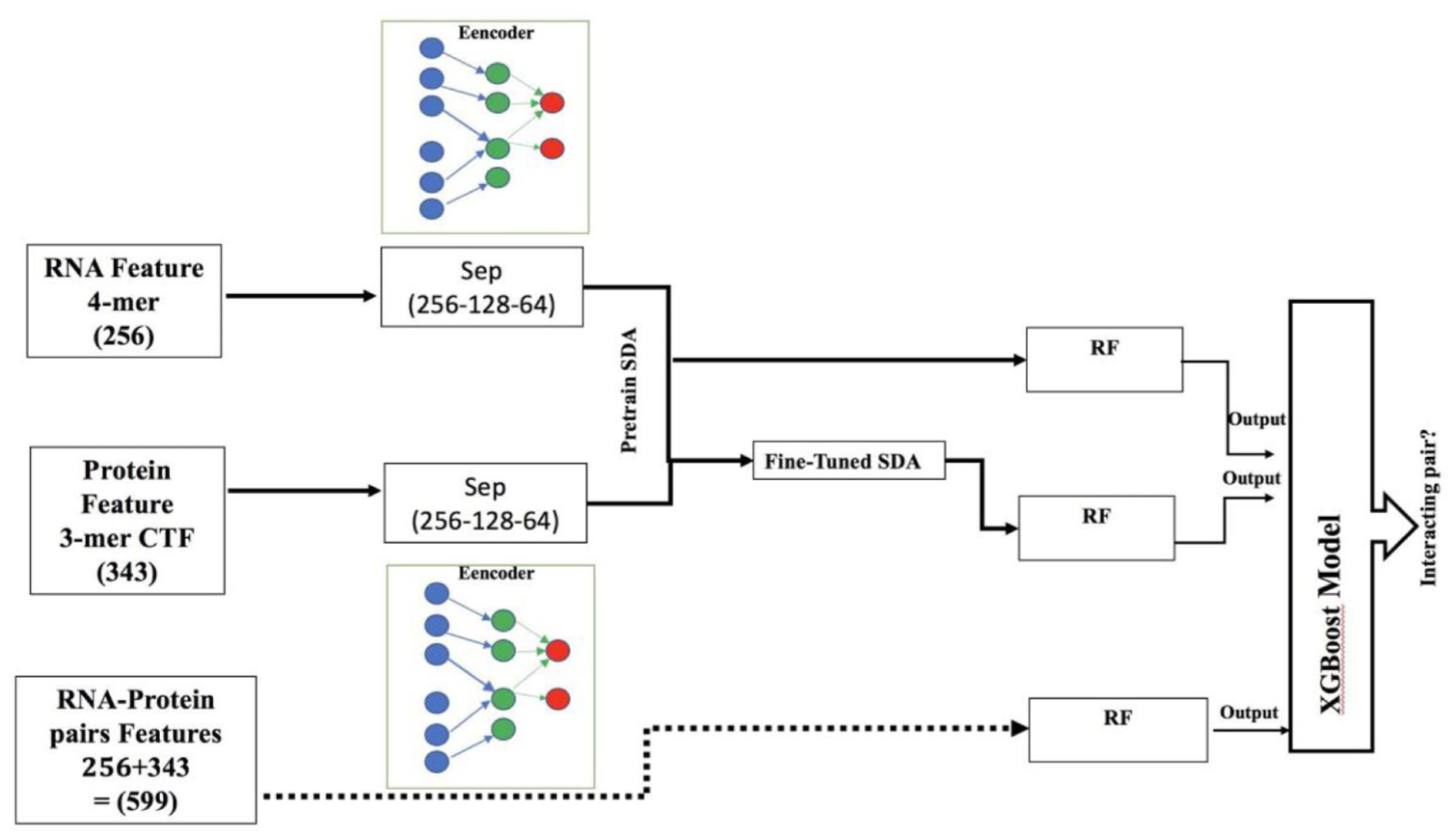
Network architecture of two separate stacked network architecture of the RPI-SDA-RF-XGBoost (sep-256-128-64).

Prediction evaluation metrics

A 5-fold cross-validation (CV) was used to assess the model’s performance and contrast it with alternative outcomes. To create a k-fold CV, the data set is randomly divided into k equal-sized parts. Next, the component of each fold from 1 to k is held out for testing, while the remaining k – 1 parts of the data sets are utilized for training. The model’s error estimates are averaged after being trained and tested k times on different fold data sets. Consequently, the model’s error rate is represented by the averaged error estimate.¹² In our research, the data is divided into 3 categories: training (70 % of the data), validation (10 %), and testing (20 %). The performance measures were produced using the following 5 parameters: Matthew’s correlation coefficient (MCC), accuracy (Acc), sensitivity (Sn), specificity (Sp), and precision (Pre). These metrics are addressed in Equations 7 to 11:

A c c u r a c y = \frac{(T P + T N)}{(T P + T N + F P + F N)}

(7)

S e n s i t i v i t y = \frac{T P}{T P + F N}

(8)

S p e c i f i c i t y = \frac{T N}{T N + F P}

(9)

P r e c i s i o n = \frac{T P}{F P + T P}

(10)

M C C = \frac{(T N \cdot T P - F N \cdot F P)}{\sqrt{(F P + T P) (F N + T P)} (F P + T N) (F N + T N)}

(11)

Here, TP, FN, FP, and TN stand true positive, false negative, false positive, and true negative, respectively.

Results

In this study, we ran extensive experiments to evaluate the efficiency of multiple machine learning models. We used 3 baseline models, namely, Naive Bayes (NB), Random Forest (RF), and XGBoost model as well as ensemble—based meta-learners for building the proposed final model.

Performance of baseline model

As shown in Figure 5, we may conclude that RF and XGBoost exceed the NB classifier in terms of accuracy across all 5 benchmark data sets. It is evident that out of all data sets, these 2 classifiers had the best accuracy.

Figure 5.

A comparison of the performance of five benchmark data sets using baseline models.

Performance of meta learner-based models

We developed 3 different meta learner-based models, namely, RPI-SDA-RF, RPI-SDA-FT-RF and RPI-SDA-XGBoost. Among them, RPI-SDA-XGBoost with Sep256-128-64, generates the best prediction results as shown in Table 4. This demonstrated that, meta learner-based models performed better than baseline models. Table 4 presents the performance of each classifier over 5 distinct benchmark data sets.

Table 4.

Performance metrics for baseline model and proposed meta-learners on multiple benchmark data sets.

Data set	Method used	Acc	Sn	Sp	Pre	MCC	AUC
RPI_369	RPI_SDA_XGBoost	0.6748	0.4609	0.8888	0.8039	0.3863	0.7299
	RPI_seq_RF (Raw feature)	0.5867	0.5611	0.6125	0.5907	0.1743	0.6699
	SDA_RF	0.6600	0.6668	0.6534	0.6603	0.3227	0.7639
	SDA_FT_RF	0.6735	0.7182	0.6288	0.6588	0.3495	0.7698
RPI_488	RPI_SDA_XGBoost	0.8873	0.8272	0.9464	0.9411	0.7822	0.8951
	RPI_seq_RF (Raw feature)	0.8849	0.8354	0.9429	0.9373	0.7852	0.9072
	SDA_RF	0.8873	0.8354	0.9388	0.9346	0.7821	0.9079
	SDA_FT_RF	0.8668	0.8312	0.9020	0.8996	0.7406	0.9074
RPI_1807	RPI_SDA_XGBoost	0.9703	0.9833	0.9540	0.9692	0.9401	0.9923
	RPI_seq_RF (Raw feature)	0.9697	0.9795	0.9575	0.9667	0.9388	0.9942
	SDA_RF	0.9696	0.9832	0.9520	0.9626	0.9389	0.9932
	SDA_FT_RF	0.9660	0.9756	0.9540	0.9672	0.9312	0.9827
RPI_2241	RPI_SDA_XGBoost	0.8353	0.7782	0.8925	0.8790	0.6755	0.8942
	RPI_seq_RF (Raw feature)	0.8273	0.8126	0.8420	0.8373	0.6550	0.9092
	SDA_RF	0.7790	0.7501	0.7631	0.7570	0.5614	0.8726
	SDA_FT_RF	0.7735	0.7858	0.7613	0.7683	0.5487	0.8686
RPI_ NPInter v2.0	RPI_SDA_XGBoost	0.9442	0.9396	0.9466	0.9463	0.8862	0.9563
	RPI_seq_RF (Raw feature)	0.9431	0.9470	0.9414	0.9418	0.8848	0.9806
	SDA_RF	0.9349	0.9448	0.9396	0.9399	0.8844	0.9798
	SDA_FT_RF	0.9223	0.9375	0.9070	0.9098	0.8449	0.9746

RPI-seq-RF is the based model. RPI- SDA-RF, RPI-SDA-XGBoost, RPI-SDA-FT-RF represents other variants of SDA models. The bold text highlights the highest-performing measure among the methods compared.

In the data sets RPI_369, RPI_488, RPI_1807, RPI_2241, and RPI_NPInter v2.0, our ensembling method did better than the other 3 base models in predicting accuracy (0.6748, 0.8873, 0.9703, 0.8353, and 0.9442, respectively). As shown in Table 4, on data set RPI_369, the SDA-RF base predictor did better than the other 2 predictors on specificity and precision. Also, SDA-FT-RF had the best than the other 2 base predictors on accuracy, sensitivity, MCC, and AUC achieving 0.6735, 0.7182, 0.3495, and 0.7698, respectively. In addition, in the RPI_488 data set, the SDA-RF base predictor did better than the SDA-RF base predictor. Accuracy was 0.8873, precision was 0.9346, sensitivity was 0.8354, specificity was 0.9388, MCC was 0.7821, and AUC was 0.9079. Also, on data sets RPI_2241 and RPI_NPInter v2.0, RPI-Seq-RF had better performance than the other 2 base predictors, SDA-RF and SDA-FT-RF. With respect to data set RPI_2241, its accuracy was 0.8273, sensitivity was 0.8126, specificity was 0.8420, precision was 0.8373, MCC was 0.6550, and AUC was 0.9092. In addition, on data set RPI NPInter v2.0, it had an accuracy of 0.9431, a sensitivity of 0.9470, a specificity of 0.9414, a precision of 0.9418, an MCC of 0.8848, and an AUC of 0. 9806. This suggests that on both structure-based and non-structure-based data sets, no one predictor outperforms others. In addition, on data sets RPI_1807, the RPI-seq-RF individual base predictor had the best on accuracy, specificity, and AUC, and the SDA-RF individual predictor had the best on sensitivity and MCC. While SDA-FT-RF base predictor had the best precision. It is quite encouraging to combine these basic predictors because this result suggested that they had a reduced correlation with the anticipated interactions. The rationale is that the accuracy of the ensemble predictor increases with the variety of the base predictors.²⁹ As you can see from Table 4, our ensemble strategy did well in the RPI_1807 and RPI_NPInter v2.0 data sets. With respect to data set RPI_1807, its accuracy was 0.9703, sensitivity was 0.9833, specificity was 0.9540, precision was 0.9692, MCC was 0.9401, and AUC was 0.9923. Similarly, about data set RPI_NPInter v2.0, its accuracy was 0.9442, sensitivity was 0.9396, specificity was 0.9466, precision was 0.9463, MCC was 0.8862, and AUC was 0.9563. According to these findings, we conclude stacked ensembling based meta-learners show enormous potential for improving the performance of RPI task.

Supplementary Figures S1 display the ROC curves for baseline model as well as all meta-learner-based models on all benchmark data sets. We achieved the best AUC values of 0.7299, 0.8951, 0.9923, 0.8902, and 0.9563 in data sets RPI_369, RPI_488, RPI_1807, RPI_2241, and RPI_NPInterv2.0, respectively for the proposed RPI-SDA-XGBoost model. The ROC curves demonstrate how well the stacked ensembling strategy of our suggested network design performs across all data sets.

Discussion

In this paper, we suggested a sequence-based encoding approach to predict ncRPIs using an SDA deep learning model with an ensembling technique. Moreover, we compared our network results with the best previous results based on 5 benchmark data sets. Then we address the limitations of our computational proposed method.

Comparison of other methods

Table 5 clearly demonstrates that our proposed network architecture surpasses the IPMiner and RPITER methods on data set RPI 369, achieving specificity and precision performance metrics of 0.889 and 0.804, respectively. On data set RPI_488, while the RPI-SAN method outperformed our proposed method with an accuracy of 0.897, it still achieved an accuracy of 0.887, outperforming the BGFE method in most performance metrics. Also, RPI-SDA-XGBoost had the same RPITER method in specificity metric as 0.947. Furthermore, on the RPI_1807 data set, the proposed method demonstrated a significant improvement in accuracy (0.970) compared with all previous methods, achieving satisfactory performance across all measurements, albeit with a slightly lower accuracy than the IPMiner method (0.986). In the RPI_2241 data set, our method reported an accuracy of 0.835, which is better than the accuracy of the IPMiner method and a little worse than the previous methods. In addition, on this data set our method outperformed all the previous methods by having a precision of 0.879. Furthermore, our architecture performed well on the RPI_NPInter v2.0 data set, particularly on precision of 0.946, compared with other methods with little accuracy disadvantage, such as IPMiner (Acc of 0.952) and RPITER (Acc of 0.955). According to the comparison results, our ensembling approach had good prediction performance, especially on data sets RPI_1807 and RPI_NPInter v2.0. Although RPI-SDA-XGBoost did not achieve the best performance among all methods in these data sets, it still has an accuracy of 0.675, 0.887, 0.970, 0.835, and 0.944 on data sets RPI_369, RPI _488, RPI_1807, RPI_ 2241, and NPInter v2.0, respectively.

Table 5.

Comparison of RPI-SDA-XGBoost against other existing models in literature.

Data set	Model Used	Acc	Sn	Sp	Pre	MCC	AUC
RPI_369	RPI_SDA-XGBoost (Sep-256-128-64)	0.675	0.461	0.889	0.804	0.386	0.730
	IPMiner	0.752	0.735	0.791	0.713	0.507	0.773
	RPITER	0.728	0.797	0.659	0.701	0.461	0.821
RPI_488	RPI_SDA-XGBoost (Sep-256-128-64)	0.887	0.827	0.947	0.941	0.782	0.895
	IPMiner	0.891	0.939	0.831	0.945	0.784	0.914
	RPITER	0.893	0.839	0.947	0.943	0.793	0.911
	RPI-SAN	0.897	0.943	0.837	0.952	0.793	0.920
	BGFE	0.887	0.927	0.835	0.933	0.774	0.898
RPI_1807	RPI_SDA-XGBoost (Sep-256-128-64)	0.970	0.983	0.954	0.970	0.940	0.992
	IPMiner	0.986	0.982	0.993	0.978	0.972	0.998
	RPITER	0.968	0.986	0.946	0.959	0.936	0.990
	RPI-SAN	0.961	0.936	0.999	0.914	0.924	0.999
	BGFE	0.960	0.934	0.999	0.912	0.922	0.992
RPI_2241	RPI_SDA-XGBoost (Sep-256-128-64)	0.835	0.778	0.892	0.879	0.675	0.894
	IPMiner	0.824	0.833	0.812	0.836	0.650	0.906
	RPITER	0.890	0.917	0.863	0.871	0.781	0.957
	RPI-SAN	0.908	0.862	0.974	0.841	0.823	0.962
	BGFE	0.913	0.877	0.966	0.859	0.834	0.947
NPInter v2.0	RPI_SDA-XGBoost (Sep-256-128-64)	0.944	0.940	0.947	0.946	0.886	0.956
	IPMiner	0.952	0.946	0.959	0.945	0.904	0.995
	RPITER	0.955	0.973	0.937	0.939	0.910	0.985

The bold text highlights the highest-performing measure among the methods compared.

Furthermore, Figure 6 shows the prediction accuracy between the RPI-SDA-XGBoost proposed method, and the previous methods based on 5 benchmark data sets. It is important to note that not all the previous studies compared on 5 benchmark data sets because it is not available. Our proposed architecture prediction accuracy performed well in all data sets. Although our method had slightly lower accuracy on RPI 369 and RPI 2241, it achieved nearly the same accuracy on RPI 488, RPI 1807, and RPI_NPInter v2.0. Proposed RPI SDA-XGBoost model achieved the best precision of 87.9% and 94.6% in the largest 2 data sets RPI 2241, and RPI NPInter v2.0, respectively.

Figure 6.

Performance comparison for RPI-SDA-XGBoost and previous DL methods.

Limitations

While our suggested approach excels computationally in predicting the interaction between ncRNA and proteins, it still faces several drawbacks and limitations. Initially, our technique extracts 343-dimensional characteristics for proteins using the 3-mer CTF approach and 256-dimensional features for RNA using the 4-mer frequency coding method. Consequently, there is still potential for development in sequence coding techniques. The widely used CTF sequence coding method generates 599 characteristics in total by counting just the 3-mer frequency of proteins and the 4-mer frequency of RNA (ie, 343 and 256). As a result, the CTF ignores the sequence information for RNA with 1-3 mers and 1-2 mers of protein. Second, we ignored the sequence structure information in favor of focusing on the main sequence information in our analysis. As such, it is worthwhile investigating more potent sequence coding techniques that efficiently combine sequence structure information with main sequence information. Furthermore, while our deep learning technique uses stacked neural networks to automatically capture high-level data, it does not offer biological insights into the relationships between ncRNAs and proteins. In addition, our computational method was excessively time-consuming since it made use of our layered ensembling methodology to improve its performance. This integrating method, which is based on a deep learning model, required a lot of time because it trained the RF classifiers 3 times on separate data sets (raw and high-level features before and after FT). This is especially true for big data sets.

Conclusion

In this study, we proposed a DL model named RPI-SDA-XGBoost to predict the potential interaction between ncRNA and protein. We utilized the 3-mer CTF frequency method to encode the protein sequence information, and the 4-mer frequency method to encode the RNA sequence information, resulting in the extraction of a total of 599-dimensional vector features. The deep learning approach is based on the SDA to extract high-level hidden features. The goal of our proposed method is to denoise the AE and train the networks to reconstruct clean input from artificially corrupted input added during training. In our proposed model, we integrated the probability outputs from the 3 base predictors to train the final XGBoost classifier as meta learners on the combined probability results from them. We assessed the performance of our suggested architecture using 5 benchmark data sets. Based on the results our model outperformed most of the individual methods and significantly improved the prediction performance compared with individual predictors on most benchmark data sets. Also, we compared our DL network architecture with the previous state-of-the-art DL methods. Our method shows powerful performance across most data sets, particularly in RPI_1807 and RPI_NPInter v2.0, and surpasses previous methods in certain performance metrics. Furthermore, our method demonstrated impressive performance in the large-scale, non-structure-based data set NPInter v2.0, a unique source of RNA-protein interaction data sets.

As a future direction, we propose additional research as follows: First, an improved CTF method could repeat the same study, extending the protein and RNA features. We can also use the pseudo amino acid composition (PAAC) descriptor, the PZM descriptor, and the bi-gram probability feature method to get feature vectors from the position-specific scoring matrix (PSSM) for protein sequences. We can also use singular value decomposition (SVD) to get feature vectors from ncRNA sequences represented by sparse k-mers matrices. Second, since our study was mostly about using sequence information to encode ncRNA and proteins, it would be also useful to combine structural information from protein and ncRNA. Third, although the extracted high-hidden-level features have a powerful ability to discriminate, they do not provide direct biological insights into ncRPIs. Therefore, to extract advanced hidden characteristics from a biological standpoint, we anticipate designing better network architecture in future study. A larger data set enhances deep learning performance by automatically learning representative features. Therefore, large training data sets are needed to account for various scenarios, including non-structure-based RPI_13254 data sets. A comparison with classical (non-AI) methods for analyzing ncRNA-Protein Interactions (eg, CatRapid and similar tools) was not done for this current paper and is open to still be tested.

Supplemental Material

sj-docx-1-bbi-10.1177_11779322251391075 – Supplemental material for A Deep Learning Model to Predict the ncRNA-Protein Interactions Based on Sequences Information Only

Supplemental material, sj-docx-1-bbi-10.1177_11779322251391075 for A Deep Learning Model to Predict the ncRNA-Protein Interactions Based on Sequences Information Only by Maha FM Sewailem, Muhammad Arif and Tanvir Alam in Bioinformatics and Biology Insights

Footnotes

Acknowledgements

The authors express their gratitude to Hamad Bin Khalifa University’s College of Science and Engineering in Qatar.

ORCID iD

Tanvir Alam

Ethics Consideration

Not required.

Informed Consent

Not Applicable.

Author Contributions

Maha F.M. Sewailem: Methodology; Writing—original draft; Software; Validation.

Muhammad Arif: Validation; Visualization; Formal analysis; Writing—review & editing.

Tanvir Alam: Conceptualization; Funding acquisition; Writing—original draft; Project administration; Formal analysis; Supervision.

Funding

The authors disclosed receipt of the following financial support for the research, authorship, and/or publication of this article: Qatar National Library (QNL), Qatar provided funding for this article’s open access publishing. The study’s design, data collection, analysis, and interpretation, as well as paper writing, were all done independently of the funding agencies.

Declaration of Conflicting Interests

The authors declared no potential conflicts of interest with respect to the research, authorship, and/or publication of this article.

Data Availability Statement

Source is made available in GitHub at https://github.com/tanviralambd/ncRNAProtein. We obtained data sets for this study from

Supplemental Material

Supplemental material for this article is available online.

References

Zhan

Jia

Zhou

HC.

BGFE: a deep learning model for ncrna-protein interaction predictions based on improved sequence information. Int J Mol Sci. 2019;20:978. doi:10.3390/ijms20040978

Alam

Al-Absi

HRH

Schmeier

Deep learning in lncrnaome: contribution, challenges, and perspectives. Noncoding RNA. 2020;6:47. doi:10.3390/ncrna6040047

Pan

Fan

Yan

Shen

HB.

IPMiner: hidden ncRNA-protein interaction sequential pattern mining with stacked autoencoder for accurate computational prediction. BMC Genomics. 2016;17:582. doi:10.1186/s12864-016-2931-8

Harrow

Frankish

Gonzalez

, et al. GENCODE: the reference human genome annotation for The ENCODE Project. Genome Res. 2012;22:1760-1774. doi:10.1101/gr.135350.111

Alam

Uludag

Essack

, et al. FARNA: knowledgebase of inferred functions of non-coding RNA transcripts. Nucleic Acids Res. 2016:gkw973. doi:10.1093/nar/gkw973

Salhi

Essack

Alam

, et al. DES-ncRNA: a knowledgebase for exploring information about human micro and long noncoding RNAs based on literature-mining. RNA Biol. 2017;14:963-971. doi:10.1080/15476286.2017.1312243

Peng

Han

Zhang

RPITER: a hierarchical deep learning framework for ncrna–protein interaction prediction. Int J Mol Sci. 2019;20:1070. doi:10.3390/ijms20051070

Musleh

Islam

Qureshi

Alajez

Alam

MSLP: mRNA subcellular localization predictor based on machine learning techniques. BMC Bioinformatics. 2023;24:109. doi:10.1186/s12859-023-05232-0

Musleh

Arif

Alajez

Alam

Unified mRNA subcellular localization predictor based on machine learning techniques. BMC Genomics. 2024;25:151. doi:10.1186/s12864-024-10077-9

10.

Muppirala

Honavar

Dobbs

Predicting RNA-protein interactions using only sequence information. BMC Bioinformatics. 2011;12:489. doi:10.1186/1471-2105-12-489

11.

Suresh

Liu

Adjeroh

Zhou

RPI-Pred: predicting ncRNA-protein interaction using sequence and structural information. Nucleic Acids Res. 2015;43:1370-1379. doi:10.1093/nar/gkv020

12.

You

Huang

Jiang

LP.

A deep learning framework for robust and accurate prediction of ncrna-protein interactions using evolutionary information. Mol Ther Nucleic Acids. 2018;11:337-344. doi:10.1016/j.omtn.2018.03.001

13.

Diao

Luo

Guo

A comprehensive survey on deep learning-based identification and predicting the interaction mechanism of long non-coding RNAs. Brief Funct Genomics. 2024;23:314-324. doi:10.1093/bfgp/elae010

14.

Lewis

Walia

Terribilini

, et al. PRIDB: a protein-RNA interface database. Nucleic Acids Res. 2011;39:d277-d282. doi:10.1093/nar/gkq1108.

15.

Huang

Jiao

Yang

, et al. LGFC-CNN: prediction of lncRNA-protein interactions by using multiple types of features through deep learning. Genes. 2021;12:1689. doi:10.3390/genes12111689

16.

Wang

Zhao

Gong

, et al. EDLMFC: an ensemble deep learning framework with multi-scale features combination for ncRNA–protein interaction prediction. BMC Bioinformatics. 2021;22:133. doi:10.1186/s12859-021-04069-9

17.

Peng

Wang

Tian

Zhou

Finding lncRNA-protein interactions based on deep learning with dual-net neural architecture. IEEE/ACM Trans Comput Biol Bioinform. 2022;19:3456-3468. doi:10.1109/TCBB.2021.3116232

18.

Shaw

Chen

Xie

Jiang

DeepLPI: a multimodal deep learning method for predicting the interactions between lncRNAs and protein isoforms. BMC Bioinformatics. 2021;22:24. doi:10.1186/s12859-020-03914-7

19.

Zhang

Jin

Kang

Predicting lncRNA-protein interactions with bipartite graph embedding and deep graph neural networks. Front Genet. 2023;14:1136672. doi:10.3389/fgene.2023.1136672

20.

Zhao

Sun

Shuai

Zhao

Shuai

Predicting potential interactions between lncRNAs and proteins via combined graph auto-encoder methods. Brief Bioinform. 2023;24:bbac527. doi:10.1093/bib/bbac527

21.

Berman

HM.

The protein data bank. Nucleic Acids Res. 2000;28:235-242. doi:10.1093/nar/28.1.235

22.

LeCun

Bengio

Hinton

Deep learning. Nature. 2015;521:436-444. doi:10.1038/nature14539

23.

Vincent

Larochelle

Lajoie

Bengio

Manzagol

Bottou

Stacked denoising autoencoders: learning useful representations in a deep network with a local denoising criterion. J Mach Learn Res. 2010;11:3371-3408.

24.

Bengio

Courville

Vincent

Representation learning: a review and new perspectives. IEEE Trans Pattern Anal Mach Intell. 2013;35:1798-1828. doi:10.1109/TPAMI.2013.50

25.

Kingma

. Adam: a method for stochastic optimization. arXiv. doi:10.48550/arXiv.1412.6980

26.

Ranzato

Monga

, et al. Building high-level features using large scale unsupervised learning. arXiv. doi:10.48550/ARXIV.1112.6209

27.

Pan

Tian

Huang

Shen

HB.

Towards better accuracy for missing value estimation of epistatic miniarray profiling data by a novel ensemble approach. Genomics. 2011;97:257-264. doi:10.1016/j.ygeno.2011.03.001

28.

Breiman

Random forests. Mach Learn. 2001;45:5-32.

29.

Kuncheva

Whitaker

CJ.

Measures of diversity in classifier ensembles and their relationship with the ensemble accuracy. Mach Learn. 2003;51:181-207. doi:10.1023/A:1022859003006

Supplementary Material

Please find the following supplemental material available below.

For Open Access articles published under a Creative Commons License, all supplemental material carries the same license as the article it is associated with.

For non-Open Access articles published, all supplemental material carries a non-exclusive license, and permission requests for re-use of supplemental material or any part of supplemental material shall be sent directly to the copyright owner as specified in the copyright notice associated with the article.

0.00 MB

0.72 MB