Advancing Regulatory Genomics With Machine Learning

Abstract

In recent years, several machine learning (ML) approaches have been proposed to predict gene expression signal and chromatin features from the DNA sequence alone. These models are often used to deduce and, to some extent, assess putative new biological insights about gene regulation, and they have led to very interesting advances in regulatory genomics. This article reviews a selection of these methods, ranging from linear models to random forests, kernel methods, and more advanced deep learning models. Specifically, we detail the different techniques and strategies that can be used to extract new gene-regulation hypotheses from these models. Furthermore, because these putative insights need to be validated with wet-lab experiments, we emphasize that it is important to have a measure of confidence associated with the extracted hypotheses. We review the procedures that have been proposed to measure this confidence for the different types of ML models, and we discuss the fact that they do not provide the same kind of information.

Introduction

Machine learning (ML) has been used for decades in genomics and bioinformatics. Among many other examples, protein modeling with hidden Markov models dates back to 1992, ¹ and the book of P. Baldi and S. Brunak ² Bioinformatics: the machine learning approach was published in 1998. In regulatory genomics specifically, position weight matrices (PWMs), which are the most common models for transcription factor (TF) binding sites, appeared in the late 1980s.^3,4 In the following years, many algorithms have been proposed in the literature to estimate the parameters of a PWM from sequence examples.^4-7 Today, PWMs of hundreds of TFs are available in databases such as JASPAR ⁸ and HOCOMOCO ⁹ and can be used to predict binding affinities and to identify potential binding sites in genomes.

In recent years, several ML approaches have been proposed to go beyond single TF binding sites, by modeling entire regulatory sequences spanning hundreds or even thousands of base pairs. These models range from linear models ¹⁰ to random forests (RFs), ¹¹ kernel methods,^12,13 convolutional neural networks (CNNs),^14,15 and more advanced deep learning approaches.^16,17 Notably, deep learning approaches adapted from methods initially developed for image and natural language processing have attracted considerable attention in the field. All these studies take place in a supervised framework, where the goal is to train a model able to predict a signal measuring gene expression (RNA-seq, CAGE, etc), TF binding, or histone marks (ChIP-seq, ATAC-seq, etc) on the basis of the DNA sequence only. Despite the supervised framework, in a large number of studies, these models are not really used as predictors. Instead, the goal is to use the model to deduce, and to some degree assess, new biological knowledge and hypotheses about gene regulation; hypotheses that have then to be experimentally validated. Along with the availability of a huge quantity and diversity of genomic, transcriptomic, and epigenetic data, these approaches have allowed very interesting progress in regulatory genomics. Maybe one of the most striking results is the fact that gene expression can be predicted with often high accuracy, albeit not perfectly,^18-20 from the sequence only, which means that a large part of the instructions for the control of gene expression likely lie at the level of the DNA. This is in contradiction with a common belief that gene expression first depends on chromatin marks that are not necessarily controlled by the DNA sequence. ²¹ Actually, several of the early works in the field have shown that epigenetic marks can be predicted from the sequence alone, often with very good accuracy.^11,13,15

Beyond this very general result, other biological hypotheses can be deduced from ML models. As we will see in this review, different strategies/methods can be used to deduce and assess interesting biological hypotheses with these models. Certain general knowledge, such as the cell specificity of a regulatory mechanism, can be quite easily tested by learning different models for different conditions and comparing their accuracy. However, for more specific knowledge, such as the DNA motifs involved in a specific regulation, we have to directly analyze the learned model, and this knowledge-extraction process is highly dependent on the model type. In addition, because this putative knowledge must be validated with wet-lab experiments (for example using CUT&RUN, ChIP-seq, or ChIP-nexus to validate the binding of a specific TF, STARR-seq to validate enhancers, etc), it is important to have a measure of importance associated with each of the extracted hypotheses. However, we will also see that the different models do not provide the same kind of importance measure. Specifically, for some models, these measures can be considered as objective, in the sense that they rely directly on the error of the model, estimated from the data. For other approaches, however, these estimates are more subjective, as they are computed solely on the basis of the signal predicted by the model, with no link to the associated error.

There are several recent reviews devoted to deep learning approaches for modeling genomic sequences.^22-25 In addition, several other articles address the problems of model interpretation in ML—see, e.g., references.^26-29 This review differs from these articles on several points: (1) it is specifically dedicated to the modeling of genomic sequences involved in the regulation of gene expression; (2) it presents a wide variety of models, without being restricted to deep learning approaches; and (3) it makes an inventory of methods and practices that can be used to extract different levels of biological knowledge from these models. This review is intended for biologists and computational biologists who are curious to know how ML can be used to deduce new biological hypothesis about gene regulation. Special attention has been paid to explaining the mathematical concepts simply and intuitively but also in a sufficiently detailed way so that readers without knowledge of ML should be able to fully understand the advantages and limitations of the different approaches. This article does not intend to provide an exhaustive list of methods and approaches that use ML to study regulatory sequences. Rather, the aim is to develop and provide the reader with the technical concepts necessary to understand this literature. Most of the works presented below have been selected either because they provide a good illustration of the type of analyses that can be done, or because they are, to our knowledge, among the firsts to introduce a specific type of ML model in regulatory genomics, or to interpret a given type of ML model.

This review is organized as follows. We first present different types of models, ranging from linear models to neural networks, for predicting chromatin features and expression signals. The following sections discuss how these models are used to infer new biological hypothesis and give some examples of knowledge that was gained from these studies. We first give a brief literature tour on the identification and prioritization of nucleotide variants. Next, we describe simple approaches that are used to assess very general hypotheses with these models. Finally, the last section is devoted to the extraction of more complex DNA features, and to the measures of importance that are associated with these features.

ML for Regulatory Genomics

Given a genome-wide experiment (RNA-seq, ChIP-seq, ATAC-seq, etc) monitoring a specific signal (gene expression, TF binding, histone mark, etc) in a specific condition (cell type, time point, treatment, etc), the aim is to learn a model able to predict this signal based on the DNA sequence alone. We have a set of sequences X = {x¹, . . ., x^N}, each sequence xⁱ being associated with a signal yⁱ. For classification problems (e.g., when predicting TF binding or histone mark), yⁱ is limited to 2 values (e.g., –1/+1) indicating whether the ith sequence is or is not bound by the studied factor in the ChIP-seq experiment. For regression problems (e.g., when predicting a gene expression signal) yⁱ is a continuous value that measures the expression associated with ith sequence (in this case, sequences may be, e.g., gene promoters or enhancer sequences). Therefore, the goal is to learn a prediction function f (x) that predicts the signal associated with sequence x. An important remark is that the function f is associated with a specific experiment and therefore with specific conditions: If the conditions change (e.g., if the cell is treated with a new drug), the function f may no longer be a good fit of the cell and another predictor should be learned from data monitoring these new conditions.

An important and difficult question that inevitably arises in classification problems is how to select the negative sequences. In general, generating random negative sequences should be avoided, even using sophisticated random models that preserve GC content or even higher levels of di- or tri-nucleotide distributions, as these sequences will always imperfectly mimic true genomic sequences. Rather, negative sequences should be true genomic sequences that have been carefully sampled for the problem or the biological question at hand. For example, if the goal is to identify the sequence features that determine the binding of a particular TF, the positive sequences will be those bound by the TF in a specific ChIP-seq experiment. For the negative sequences, several options will be available¹¹: We could use unbound sequences of the same type as those used in the positive set (e.g., originating from promoter and enhancer sequences, using the same proportion as observed in the positive sequences). Another possibility would be to use sequences with similar epigenetic contexts (i.e., similar histone marks or similar chromatin opening marks), or sequences that are not bound by the TF of interest but that are bound by other TFs in the same cell type. The choice of negative sequences usually has a large impact on the measured accuracy of the model, and for this reason, it is often difficult to compare the accuracy of different ML approaches, even when they are applied to data from the same experiment. On the contrary, as we will see in the following, the choice of the negative sequences is one of the convenient tools at our disposal to derive new biological knowledge using ML.

Note that even when the purpose of the study is not to make predictions per se, the prediction framework keeps several interests: First, in comparison to simple correlation analyses that can also identify some links between sequence features and the target signal, predictive models enable the combination of several DNA variables and hence reveal cellular mechanisms that cannot be studied with simple correlation analyses. Second, when estimating the accuracy of the model we also assess the amount of information that has been captured by the model—and, maybe more importantly, what remains to be captured. To avoid any optimistic bias, a golden rule in ML is that the accuracy estimate must be computed on left-out sequences, i.e., positive and negative sequences that were not used to train the model. These sequences are called test sequences, as opposed to the training or learning sequences. Another important issue is the choice of the measure of accuracy. For regression problems, a popular choice is to compute the correlation between measured and predicted signals on the test sequences, although alternatives such as the percentage of variance explained are also often used. For classification problems, the most popular choices are the area under the receiver operating characteristic (ROC) curve (AUROC) and the area under the precision-recall curve (AUPR), see Box 1.

Box 1.

Measures of accuracy for classification problems.

In classification problems, ML approaches often learn a prediction function f(x) that returns a real-valued output y. The returned value is then used to predict the class (–1 or +1) of the example x by applying a predefined threshold t: If y ≥ t, then x is classified as +1; otherwise, x is classified as –1. Given a predictor f and a threshold t, we can estimate several statistics related to the accuracy of the predictions:  • The true positive rate (TPR, or recall) is the proportion of positive examples of the test set that are predicted as positive, i.e., for which f(x) ≥ t.  • The false positive rate (FPR) is the proportion of negative examples of the test set that are (erroneously) predicted as positive.  • The precision is the proportion of examples predicted as positives that are really positives. Precision and recall (TPR) are usually antagonistic statistics: When one increases, the other one often tends to decrease. The above statistics depend on the threshold t used to classify an example as positive. As the value of this threshold actually depends on the problem at hand (in some classification problems, we may prefer to have a high recall, whereas, in others, a high precision is more important), the accuracy of a predictor is usually measured using ROC or precision-recall curves:  • The ROC (receiver operating characteristic) curve plots the TPR as a function of the FPR, by varying the threshold t. The area under this curve (the AUROC) is a statistic that summarizes the whole curve, with an AUROC of 1 corresponding to a perfect classifier that would classify all true positives as positives, and all true negatives as negatives. On the opposite, random predictors, as well as predictors that always predict the same class, have an AUROC of 0.5.  • The precision-recall (PR) curve plots the precision as a function of the recall (TPR). As for the ROC, perfect classifiers have an area under the PR curve (AUPR) equal to 1. The AUROC is sometimes erroneously presented as being biased for unbalanced problems, i.e., problems where the negative sequences outnumber the positive ones. Actually, one property of the ROC is that it is insensitive to these numbers, which means that a given predictor will have exactly the same ROC (and hence AUROC) regardless of the proportion of positives among all sequences (90%, 50%, 5%, . . .). On the contrary, the precision is highly dependent on this proportion, and the same predictor will have decreasing precision values as the proportion of negative sequences increases. Therefore, if the predictor is really aimed at predicting the classes of new sequences, the AUPR may be a better statistic than the AUROC, as monitoring the precision is important in this case. On the contrary, if the goal is to quantify the amount of biological knowledge gained by the model regardless of the proportion of positives/negatives, the AUROC is a convenient measure.

In the following, we present different types of methods that have been proposed in this context: support vector machines (SVMs), RFs, linear models, and CNNs.

Support vector machines

One of the first studies dedicated to the prediction of ChIP-seq signal based on long regulatory sequences was the kmer-SVM approach, ¹² latter upgraded in gkm-SVM. ¹³ SVMs are among the most successful methods of ML. ³⁰ They work by searching for a hyperplane that best separates the training examples according to their classes. However, rather than searching for a hyperplane in the original space of the data, SVMs work in a usually much higher dimensional space (with possibly infinite dimension). As a result, although the separating hyperplane is by definition linear in the enlarged space, it can define non-linear boundaries in the original space (see Figure 1). The beauty of SVMs is that we do not need to define the enlarged space. The only thing we have to define is a kernel function that measures the similarity of any pair of examples. The “trick” is that the position of a new example relative to the separating hyperplane can be computed by a linear combination of the similarity of this new example with all training examples, i.e.:

$$f\left(x\right)=b+\sum _{i=1}^N{\alpha }_i{y}^{i}K(x,x^i),$$

(1)

with b and α_i the parameters of the SVM estimated by the learning algorithm, yⁱ the class of the ith sample of the training set (–1 or +1), and K(x, xⁱ) the result of the kernel function between sample x and the ith example of the training set. The sign of f (x) gives us the position of x relative to the hyperplane (up or down) and hence the predicted class of the sample. Moreover, only some training examples are associated with an α_i different from 0 (the so-called support vectors), so, in practice, Expression (1) is computed without the need to compute the kernel function for all training examples.

Figure 1.

SVMs work in enlarged spaces. A toy example, illustrating the fact that a linear model in an enlarged space (the gray plane in the 3D space on the right) can define non-linear boundaries in the original space (the gray ellipse in the 2D space on the left), thus providing an accurate classifier for the 2 point classes (red vs. green).

Thus, the accuracy of the approach depends on the chosen kernel function K(x, x^′) which must be meaningful for the problem at hand. The authors of kmer-SVM ¹² proposed a kernel function based on the similarity of the k-mers present in the sequences. More formally, each sequence x is encoded by a vector that reports the number of occurrences of each of the 4^k k-mers in x (for a given size k). Sequence pairs that have the same relative frequency for each k-mer have K(x, x^′) = 1, whereas sequences that do not have any k-mer in common have K(x, x^′) = 0. The method has been improved a few years later by the gkm-SVM approach that uses gapped k-mers (i.e., k-mers with a certain number of non-informative positions for which any nucleotide is possible), ¹³ but the principle remains the same: Training sequences that most resemble the new sequence x in terms of (gapped) k-mers composition have more weight in Expression (1) and drive the predicted class toward their own class. The gkm-SVM approach has been applied to 467 human ChIP-seq experiments from the ENCODE project. ³¹ For each ChIP-seq experiment, sequences associated with a ChIP-seq peak were extracted and used as positive sequences (authors report an average sequence length of around 300 bps), whereas the same number of random genomic sequences were used as negative sequences. Then, an SVM (one for each ChIP-seq experiment) was learned to discriminate between these 2 sets, and the accuracy of each of these 467 SVMs was estimated by the AUROC (see Box 1). The approach showed AUROC above 80% on the test set for most ChIP-seq experiments.

Random forests

Another method that has been proposed for the prediction of ChIP-seq signal is RFs. ¹¹ RFs ³² had considerable success and attention in the ML literature in the last 20 years. RFs are an extension of decision trees, which are certainly among the oldest approaches in ML. ³³ A decision tree encodes a set of tests that can be done on the features of a given example to predict its class (see Figure 2). As the name suggests, these tests are organized in a tree structure that provides the order in which the tests are done (from the root to the leaves). Each node corresponds to a binary test on a specific feature of the samples (e.g., “is feature #3 > 0.66?”), and the 2 edges that follow the node correspond to the 2 possible outcomes of the test. Thus, each path from the root to a leaf corresponds to a series of tests that lead to the prediction of the class associated with that leaf (which is the majority class of the training examples that belong to this leaf). Learning a decision tree involves deciding the tests associated with each node (typically which feature and which threshold on this feature?), and several algorithms have been proposed to build trees with minimum prediction error. Decision trees are accurate on certain problems and have the great advantage of being simple to understand and interpret. However, they are known to be quite unstable (a slight change in the training data can lead to very different trees) and they can be relatively inaccurate on some problems. ³² Random forests have been proposed to overcome these issues, at the price, however, of an indubitable loss of readability. An RF is a combination of many (sometimes hundreds or even thousands) decision trees. All these trees are independently learned on the same problem, with a dedicated algorithm that integrates a stochastic procedure to ensure that all trees are different. Once learned, the RF can be used to predict the class of a new sample with a very simple procedure: Each tree is used to predict the class, and the most popular class is proposed by the forest. This voting scheme removes the instability problem, and, if the learned trees are sufficiently independent, the accuracy of the forest can be much higher than that of single trees ³² .

Figure 2.

A toy decision tree inspired from the Epigram method. ¹¹ The learning set involves 1000 sequences (500 positive + 500 negative, see left table). Each sequence is described by the score of 50 PWMs. The decision tree learned from these sequences encodes a set of rules that classify a sequence as positive if the score of PWM#5 is > 80, or if the score of PWM#12 and #21 are > 70 and 85, respectively. Numbers at the top of each node provide the repartition of training sequences in the 2 classes.

The Epigram approach ¹¹ uses RFs to predict the presence of 6 histone marks in different human cell types from DNA sequences. An RF is learned for each mark based on the peaks identified by dedicated ChIP-seq experiments. Sequences associated with the peaks were used as positive sequences (sequence length is around 1000 bp). Negative sequences were genomic regions not covered by a peak, with different strategies for the selection. Before learning an RF, a de novo motif finding algorithm was applied to the training sequences to identify motifs that are more present in one class than in the other. Then, each sequence was described by the score obtained by the different motifs, and the RF learning algorithm was run on these data. As for SVM, the accuracy of the approach was measured by the AUROC, with accuracy above 80% for most histone marks and cell types.

Linear and logistic models

Logistic models are one of the oldest and most used approaches for binary classification problems. For a given example x = (x₁, ..., x_M) described by M variables, a logistic model expresses the probability that x belongs to the first class with a linear expression

$$P(1|x)=S\left(a+\sum _{i=1}^M{b}_i·x_i\right),$$

(2)

where P (1|x) is the probability that example x belongs to the first class, S is the sigmoid function, and a and b_i are the regression coefficients that constitute the parameters of the model. Although being quite simple, logistic and generalized linear models have gained considerable interest in domains with high-throughput data (like genomics), thanks to the development of modern regularization methods. ³⁴ For problems with a high amount of data, and in situations where the number of variables—i.e., M in Expression (2)—may be larger than the number of examples, these models can be trained very quickly and without being much affected by over-fitting. The LASSO penalty especially ³⁵ is a powerful regularization technique that allows one to train a model and select the most important features at the same time—ie, many regression coefficients of Expression (2) (a and b_i) are set to zero by the learning algorithm—which is of obvious interest when we are also interested to understand how a predictor works. ³⁶

As for SVMs and RFs, the accuracy of the approach essentially depends on our ability to provide to the learning algorithm a set of variables that contains meaningful information for the discrimination problem. For example, our group proposed such an approach to predict TF binding with a logistic model named TFcoop. ¹⁰ In TFcoop, each sequence was described by the affinity scores of all PWMs of the vertebrate JASPAR database ⁸ and the relative frequency of every dinucleotide. Affinity scores and dinucleotide frequencies were computed on 1 kb sequences. The data thus resemble that used in Epigram, ¹¹ except that in this latter the PWMs were trained de novo, and the dinucleotides were not used as predictive variables. TFcoop was applied on 409 ChIP-seq experiments from ENCODE. The positive sequences were either the promoters (±500 bp around the TSS) or the enhancers (±500 bp around the peaks defined by the FANTOM5 project) ³⁷ with a peak in the studied ChIP-seq experiment, whereas the negative sequences were the promoters or enhancers without a peak. The accuracy was assessed by the AUROC, and was similar to that of a CNN approach named DeepSea (see below) on the same problem.

Convolutional neural networks

Deep learning has shown considerable success in image recognition and many other domains, including biology and regulatory genomics. It has also led to very interesting developments in ML theory, by showing that models with a number of parameters largely exceeding the number of learning examples can be trained in certain conditions without being affected by the so-called over-fitting problem.^38,39 The simplest form of neural networks is the feedforward neural networks (see Figure 3A). These networks are defined by a (potentially very large) set of neurons, inter-connected and organized in layers. The first layer is connected to the input values of the network, whereas the last layer encodes its output. In the classical feedforward network, each neuron takes in input the output of the neurons of the previous layer (hence these layers are often referred as fully connected). It then computes a weighted sum of these values using its own set of weights, applies a simple activation function that realizes a non-linear transformation of this sum, and dispatches the computed value to the neurons of the following layer. When new values are applied to the input layer of the network, the outputs of all neurons are computed iteratively layer by layer until reaching the last one. For classification problems, the last layer is usually composed of a single neuron that produces a value in between 0 and 1 representing the probability that the example provided in input belongs to the positive class. The architecture of the network (the number of layers, neurons, and all the connections between them) as well as the set of weights associated with each neuron and the form of the activation functions define the parameters of the network. As for other ML approaches, specialized learning algorithms are used to train a neural network by minimizing its prediction error on learning examples.

Figure 3.

Neural networks. (A) An example of feedforward network with 4 layers. The first layer is connected to 9 input values (in black). The last layer involves a single neuron that outputs a value between 0 and 1. The width and color of the lines represent the weights and signs associated with the inputs to each neuron. (B) An extract of a convolutional neural network that scans DNA sequences. The input sequence is encoded as a 1-hot matrix. A filter of length 5 scans the inputs and computes a convolution at each position. The figure shows 2 convolutions done at 2 different positions with the same filter; filter weights that are associated with non-null input values in the convolution operations are overlined in black. A non-linear activation function then filters the convolution results by removing all values below a given threshold. Finally, the results of these operations are pooled by groups of 4, reducing the output of the convolution to only 4 values. In the figure, only 1 filter is represented, although each convolution layer usually involves dozens or hundreds of filters with their own activation and pooling operations. The results of all filters are then combined in the following layers of the network (not represented here).

In regulatory genomics, most neural networks are CNNs. Contrary to simple feedforward networks, CNNs also embed specific neurons called filters that realize convolutional operations (see Figure 3B). This operation is very similar to the weighted sum of classical neurons, except that the sum does not involve all neurons of the previous layer but only a small group of adjacent neurons (typically a dozen). The operation is repeated at each position of the previous layer, moving the filter 1 position at a time. Because the same filter is applied to every position of the previous layer, convolution filters effectively constitute a way to reduce the number of parameters of the model when the same local operations are applied to different regions of a layer. Hence, 1 filter produces a number of outputs that are roughly equal to the size of the previous layer. As with classical neurons, the parameters of the filters, i.e., their sizes, forms, and weights, must be inferred by the learning algorithm. Convolutional neural networks typically possess 1 or several convolutional layers. Each layer involves several convolutional filters that are applied in parallel. As for classical neurons, all outputs of a convolutional filter are run through a non-linear activation function. Contrary to classical neurons, however, this step is often followed by a pooling function that summarizes (pools) several adjacent outputs. One of the most common pooling functions is max pooling, which simply takes in input a number N of adjacent outputs of the filter, and returns a single value corresponding to the maximum of these values, thus decreasing the input size (see Figure 3B). This operation not only reduces the number of parameters of the neural network but also inevitably induces a loss of resolution, which may be impactful, e.g., when modeling TF interactions as these often occur at base-pair resolution.

Contrary to the above ML approaches, the big interest of CNNs is that they take raw data in input and directly learn the most interesting features for discriminating the 2 classes, by way of the filters of the convolutional layers. In regulatory genomics, the raw data is the DNA sequence (or RNA in certain cases). As CNNs only work on numbers, the sequence is 1 hot encoded by replacing each nucleotide with a boolean vector of size 4 (e.g., A, T, G, and C are encoded as 1000, 0100, 0010, and 0001, respectively). Hence, a DNA sequence of length M is encoded as a 4 × M boolean matrix (see Figure 3B). The CNNs used for regulatory genomics have usually 1 or more convolutional layers, followed by several fully connected feedforward layers. The filters associated with the first layer are thus directly applied to the sequence and can be viewed as models of DNA motifs. Actually, the weighted sum of a filter defines exactly the same operation as the function used to compute the score of a sequence for a given PWM. Hence, mathematically speaking, the filters of the first layer are nothing more than a set of PWMs that are applied at each position of the sequence. All these scores are then combined in the following layers, which allows the network to represent potentially any motif combination.

One of the first CNN approaches proposed for regulatory genomics was DeepBind. ¹⁴ The authors designed a CNN with 1 convolutional layer, followed by a pooling layer and a feedforward network that combines the scores of the different filters. The network was trained on many datasets measuring the binding of various DNA and RNA-binding proteins (PBM, SELEX, ChIP/CLIP). Notably, it was trained on 506 ChIP-seq data from the ENCODE project. ⁴⁰ Positive sequences were 101 bp sequences associated with a ChIP- seq peak, whereas the negative sequences were obtained by randomly shuffling the dinucleotide of the positive sequences. As for previous approaches, the accuracy of the CNNs was estimated by the AUROC.

The same year, Zhou and Troyanskaya ¹⁵ proposed another CNN approach named DeepSEA. DeepSEA has 3 convolutional/pooling layers followed by a fully connected layer. It was applied to 690 TF binding profiles, 125 DHS profiles, and 104 histone-mark profiles from ENCODE and the Roadmap Epigenomic projects.^40,41 For each predictor, the positive sequences were the sequences associated with the mark, whereas the negative sequences were randomly selected among the sequences that were not associated with the mark but that were associated with another mark in another data. CNN accuracies were estimated by the AUROCs. DeepSEA takes input sequences of 1 kb length, much longer than DeepBind (100 bp) but very similar to the size of the sequences used by Epigram (see above), and reports median AUROC in between 85% and 95% depending on the type of profiles

Following DeepSEA, Quang and Xie ¹⁶ proposed DanQ. DanQ has a single layer of convolutions that identify the motifs present in the input sequence, but this convolution is followed by a layer of recurrent neural network known as long short-term memory (LSTM). As for convolutional filters, in a recurrent network, the same function is applied to every input. However, contrary to CNN, this function also has a memory of its previous outputs. In this way, the computed output value depends both on the current input and on the previous outputs. In DanQ, the LSTMs take in input the result of the convolution filters at every position of the sequence. Hence, the output of the LSTM depends both on the value of the filters at the current position and on the output of the LSTM at the previous positions. Moreover, DanQ implements 2 LSTMs: one that reads the sequence forward, and one that reads the sequence backward. The LSTM layer is then followed by a fully connected layer. DanQ was applied exactly to the same data as DeepSea. Its accuracy, measured by AUROC and AUPR, showed a slight but constant improvement over DeepSea.

Rather than addressing a simple classification problem where the aim is to predict whether or not a sequence has a specific mark/TF, several other CNN approaches have been proposed to predict the read coverage along the sequence, i.e., the expected number of reads at each base pair.^42-45 This was the approach used by BPnet ⁴² for example. According to its authors, training the model on the entire profile enables them to capture subtle regulatory features that are not captured when training on binary signal, a behavior also reported in reference. ⁴⁴

Numerous other CNN approaches have been proposed in the following years to predict TF binding and chromatin marks, but also gene expression signal, from the sequence. Although former approaches used sequence lengths that rarely exceed 1000 bp, a clear tendency of the following approaches was to propose new architectures that can handle increasing sequence lengths to capture long-range interactions with distant regulatory sequences (enhancers/silencers).

In 2018, Zhou et al ⁴⁶ proposed the ExPecto approach, which capitalizes on the DeepSea method. ¹⁵ The approach involves 3 steps. (1) A CNN model similar to that used in DeepSea is learned on 2002 genome-wide histone marks, TF binding, and chromatin accessibility profiles (data from ENCODE and Roadmap Epigenomics projects). (2) These 2002 model tracks are used to scan 40 kb regions centered on gene TSSs. The score of these tracks at 200 positions along the 40 kb sequences provides a very large set of 200 × 2002 features describing each gene. This set is reduced to 10 × 2002 features by a spatial transformation that uses exponential decay functions. (3) These features are used as input to train different linear models that predict the RNA-seq signal associated with each gene in 218 tissues and cell types (selected from GTEX, ⁴⁷ ENCODE, and Roadmap Epigenomics projects). In each experiment, the accuracy of the model was measured by the correlation between the predicted and measured RNA-seq signal. ExPecto shows prediction accuracy with a median 81.9% correlation across the 218 models.

Another CNN approach proposed in 2018 was Bassenji. ⁴⁸ The model takes very large sequences of 131 kb in input. The network uses standard convolution/pooling layers, followed by dilated convolution layers. Contrary to standard convolutions that realize a weighted sum on the output of adjacent neurons of the previous layer, in the dilated convolution, the sum involves neurons spaced by several positions. Moreover, the network involves several dilated layers with gaps increasing by a factor of 2, which enables the model to potentially capture combinations spanning an exponential number of bps. The approach was applied not only to various DNase-seq and histone modification ChIP-seq but also to 973 FANTOM5 CAGE experiments. For these latter, the goal was to predict the CAGE signal measured on 128 bp sequences associated with a TSS. The accuracy was measured by the correlation between the measured and predicted signal and the authors report an average correlation of 85%.

Besides pure CNN approaches, one of the most recent developments in the field was the Enformer approach ⁴³ that uses self-attention techniques developed for natural language processing. ¹⁷ The Enformer model uses several standard convolutional layers to identify motifs in the input sequence. The output of these convolutional layers then goes through several multi-head attention layers that share information across the motifs and can model long-range interactions, such as those between promoters and enhancers. Enformer uses very long input sequences of 196 kb and predicts 5313 and 1643 different genomic signals (DNAse, ChIP-seq, and CAGE expression data) for the human and mouse genome, respectively.

Identifying and Prioritizing Genomic Variants

Maybe one of the most common applications of ML, and especially deep learning, for regulatory genomics has been the identification and prioritization of genomic variants from genome-wide association studies (GWAS) and expression quantitative trait loci (eQTL) studies. Genome-wide association studies use statistical methods to identify genetic variants associated with common diseases and traits. This involves the analysis of thousands of variants in large cohorts of individuals, often split into cases and controls, to identify variants associated with the trait of interest (i.e., genomes with this variant have often this trait/pathology). Similarly, eQTL studies identify associations between genomic variants and the expression of specific genes (genomes with this variant often show over-expression of gene X). GWAS and eQTL studies have identified thousands of variants statistically associated with a physiological trait or an expression profile, which are available in dedicated databases.^49,50 However, because variants are not independent (an effect called linkage disequilibrium), many variants are often present together in the same genomes. As a consequence, it is widely believed that only a few GWAS or eQTL variants are truly causal. ⁵⁰ In these conditions, an interesting idea is to use the ML models described above for the identification and prioritization of causal variants. In its simplest form, the procedure involves taking a specific model—predicting, e.g., if a sequence is bound by a given TF—and computing the prediction of this model at a given locus using (i) the reference genome and (2) the mutated genome associated with a specific variant (e.g., a specific SNP). Variants that increase or decrease significantly the predicted signal are more likely to have a strong effect on the cell and hence to be causal.^{14-16, 46} Using this principle, the authors of DeepBind proposed a new genomic representation called mutation maps to visualize the effect that every possible point mutation in a sequence may have on binding affinity. ¹⁴

More sophisticated approaches have also been proposed to identify variants using a combination of ML models. For example, a deep learning model that uses the score of ∼600 DeepBind TF models has been trained to discriminate between high-frequency variants (assumed as neutral) and disease-associated variants from GWAS studies. ¹⁴ This model takes in input the score of the ∼600 DeepBind models both for the wild-type sequence (reference genome) and the mutant sequence. Similarly, a boosted logistic regression classifier and a boosted ensemble classifier have been trained to discriminate between high-frequency SNPs and putative disease-associated variants from GWAS and eQTL studies using the epigenetic-mark predictions of DeepSea and DanQ, respectively.^15,16

Finally, it is important to note that several recent studies highlighted the limitations of state-of-the-art approaches for predicting the effect of personal variants.^18-20 Specifically, although approaches such as Enformer ⁴³ or Bassenji ⁴⁸ can quite accurately predict gene expression levels across genes in different cell types, they show some limitations to explain expression variation between individuals.^19,20 Furthermore, despite the use of very wide sequence windows (196 kb for Enformer), their ability to account for the effect of distal enhancers when predicting gene expression still appears limited. ¹⁸

Assessing Regulatory Hypotheses with ML Models

Besides the prioritization of genomic variants, the ML approaches presented here, along with many others and the concordant development and availability of various omics data, have enabled several advances in regulatory genomics over the past decade. For this, the supervised framework offers the possibility to test various hypotheses by simply training a model and estimating its accuracy on specific problems. This can be done in various ways. One approach is to directly control the nature of the input of the model. For example, Agarwal and Shendure ⁵¹ studied the size of the promoter sequences using the Xpresso model. Xpresso is a CNN model that takes in input sequences of –7/+3.5 kb centered on the TSS. In their study, the authors showed that although the large sequence –7/+3.5 kb around the TSS provides the best accuracy, most of the promoter information for the control of mRNA expression likely lies in –1.5/+1.5 kb because this sequence provides approximately the same accuracy as the longer –7/+3.5 kb. Similarly, our group studied the importance of long-biased sequences in the control of gene expression using the DExTER approach. ⁵² DExTER is a linear model that aims to predict mRNA levels based on the presence of long sequences enriched for a specific short k-mer (e.g., TAA) around the gene TSS, excluding any other information such as TFBS motifs. The approach has been applied to various eukaryotes in different cell types and conditions. For the malaria parasite, the approach showed a surprising accuracy of more than 70% correlation between measured and predicted expression, suggesting that long-biased sequences may play a predominant role in controlling gene expression for this organism.

Another procedure to test different hypotheses is to control the way positive and negative examples are selected. For example, Zheng et al ⁵³ study TF binding with a CNN. The originality of this study is that the sequences are selected in a way that ensures that the TF motif is present in both the positive (bound) and negative (unbound) sequences. In this way, the predictive model cannot simply use the presence/absence of the target motif to discriminate the sequences, and the good accuracy of the approach showed that other features are likely involved in the binding site recognition mechanism of the studied TFs. To go one step further, the authors restricted all sequences to be within DNaseI hypersensitive sites (a mark of accessible chromatin). They trained a new model and observed a drop in the accuracy, suggesting that DNA features related to open chromatin are likely involved in this recognition process.

Rather than controlling the sequences used for learning the model, another simple technique that can be used to test some hypotheses is to compare the accuracy achieved by a given model on different sets of sequences. For example, Agarwal and Shendure ⁵¹ studied the impact of enhancers on the prediction of Xpresso. Xpresso only uses the sequence located around the TSS for the prediction and hence cannot handle distal regulatory elements. Given that enhancers are frequently associated with large domains of H3K27Ac activity, the authors identified a set of 4277 genes that overlap H3K27Ac marks and observed that the predicted expression level on these genes is markedly smaller than the measured expression, a trend that was not observed for the other genes. Thus, the expression of genes under the control of enhancers seems to be underestimated by the Xpresso model, which could therefore provide a coarse filter to help identify these genes.

Finally, a very useful tool available in the ML toolbox is swap experiments. Model swapping is used to test hypotheses related to the specificity of a regulation mechanism. The procedure involves learning different models on different conditions (says conditions A and B) and comparing the accuracy of the model learned on A when it is applied to B, to the accuracy of the model learned and applied on B. In practice, an important point to which practitioners must pay close attention is that the sequences used for testing in one condition were not used for training in the other one, to avoid any bias in the accuracy estimates during swaps. This technique was extensively used in the TFcoop analyses. ¹⁰ Given 2 ChIP-seq experiments targeting the same TF in 2 cell types, a TFcoop model predicting whether a sequence is bound or not by the TF was learned for each cell type. Then the 2 models were swapped. In some cases, both models got the same accuracy, but for some TFs, the model learned on cell type A was not as good on cell type B as the model directly learned on cell type B, meaning that the rules governing the binding of the TF were not the same in the 2 cell types. Similarly, for a given ChIP-seq experiment, a model was learned for enhancer sequences and another model for promoter sequences. The swap experiment revealed that the 2 models are generally not interchangeable, and hence that the rules are different depending on the nature of the regulatory sequence (promoters vs. enhancers). On the contrary, models for mRNA promoters, lncRNA promoters and pre-miRNA promoters appeared to be perfectly interchangeable. Agarwal and Shendure ⁵¹ also did swap experiments between human and mouse. Namely, they trained one Xpresso model on mouse and one on human using comparable RNA-seq experiments and observed on a set of orthologous genes that the model learned on mouse has the same accuracy on human as the model directly learned on human (and conversely), meaning that the regulatory principles are likely very close in both organisms.

Breaking the Regulatory Code: Interpreting ML Models

Finally, the most ambitious application of ML is obviously to break the regulatory code and determine the rules used by the cell to regulate expression. A first step toward this goal is to identify all regulatory elements involved in the regulation process in question. Note that the term regulatory element has to be understood in its broadest sense here. It may stand for standard motifs of TF binding sites, but it can also refer to other features known to be involved in gene regulation, like low complexity regions such as short tandem repeats, ⁵⁴ or long-biased sequences like CpG islands, ⁵⁵ as well as any other kind of “sequence patterns” that we can think of, such as, e.g., the DNA shapes. ⁵⁶ In addition to the regulatory elements, breaking the regulatory code also means determining how these elements are combined, and what rules they follow in terms of repetition, position, and orientation on the DNA sequence. Getting down to this level of detail involves analyzing the learned model to understand how it works. This is referred to as model interpretation in the ML community. There are several definitions of interpretability in the ML literature, and these definitions are often considered domain-specific.^27,28,57,58 In the context of regulatory genomics, model interpretation has also several meanings, and we will see that the term covers different approaches that do not provide the same kind of information. The general problem is as follows: We have a predictive model that has been learned for a specific problem, and we want to understand how it works. There are at least 3 different ways to attempt this. The first and more direct approach is to explain the model by analyzing its different components and extracting the rules used to make its predictions. A second approach is to explain the predictions of the model rather than the model itself, i.e., given a sequence and a prediction, we want to explain why the model predicts this value for this sequence. A third alternative is to try to explain the model by exploring its behavior on synthetic sequences. Theoretically, the 3 approaches are possible for any type of model. However, as we will see, linear models and RFs can often be partially explained by a direct analysis of their components. For CNN models, on the contrary, this is more difficult to do, which is why different methods belonging to the second and third categories have been developed.

Explaining model components

In some cases, the model may be simple enough to be directly analyzed as a whole. This view of interpretability argues for simple and sparse models (i.e., with few parameters). This may be possible for some very small decision trees and linear models, but this is generally not the case for the regulatory models described above. Moreover, even for a simple linear model, it is known that interpretation is not obvious, as the sign of the coefficient associated with a specific variable (which is tempting to interpret as the sign of the association between this variable and the predicted signal) may change depending on the identity of the other variables included in the model.

A less stringent view of interpretability corresponds to models that can be broken down into different modules that are further analyzed.^27,28 For regulatory genomics, this corresponds to the case where we can extract the DNA features used by the model for its predictions. Note that a DNA feature may be more complex than simply the identity of a regulatory element. For example, in the DExTER method, the predictive features also encode information about the position of the regulatory elements on the DNA sequence. ⁵² Hence, DNA features may potentially encode complex information related to the number of repetitions, position, and orientation of regulatory elements on the DNA sequence. Obviously, extracting the DNA features used by a model is relatively easy to do for all models that directly take these DNA features in input, such as logistic/linear models and RFs. On the contrary, for CNN approaches the task is more difficult as we will see below.

RFs and linear models

In these models, extracting the DNA features involves identifying which variables provided in the input are the most important for the predictions. ExPecto is an example of a linear model where such interpretation is quite easy. ⁴⁶ In this article, the authors observed that, in most cases, the ExPecto models predict expression with features related to TFs and histone marks, but not with DNase I sequence features. Note that the DNA features extraction may be further facilitated if the learning algorithm directly includes a feature selection procedure such as the LASSO,^35,36 which drastically decreases the number of predictive features used by the model.

Rather than simply providing the list of features used by the model, it is much more useful to also provide a measure of importance associated with each feature.^59-61 For RFs, this is usually done by shuffling the values of each variable. Namely, the accuracy of the model is first estimated on the test set. Then, the values of the ith variable are randomly shuffled, and the loss of accuracy induced by this noise is used as a measure of the importance of the ith variable in the model.^32,61 By repeating this process, the relative importance of each variable is estimated. A very similar procedure also exists for linear/logistic models. In this procedure, the value of the coefficient associated with the ith variable is set to zero (which is equivalent to simply removing this variable from the model) and, as for RFs, the loss of accuracy induced by this operation is used as a measure of variable importance. In both cases, this measure can be considered objective, as it is based on the loss of accuracy when removing information carried by each variable. Note, however, that this approach (as all other methods described below) assesses the importance of a feature for the model, but not necessarily its importance in the cell. For example, if 2 TFs have similar PWMs (which is quite common), the model may erroneously give all the importance to one of the TF and none to the other one (see the “Conclusions” section for a discussion about this point). Nevertheless, it is an effective and useful approach to assess new biological hypotheses in silico. It has been extensively used for analyzing the binding differences of 1 TF in 2 different conditions (e.g., 2 cell types or 2 treatments), or of 2 paralogous TFs with similar PWMs using the TFscope approach. ⁶² TFscope is a logistic model that integrates 3 kinds of variables that model (1) the core motif, (2) the nature and position of binding sites of co-factors, and (3) the large nucleotidic environment around the core motif. The importance of each feature in the different comparisons was assessed with the importance measure described above. For comparisons involving 1 TF in 2 conditions, the co-factors, and to a lesser extent the nucleotidic environment, were often (but not always) the most important features explaining the differences of binding sites. For paralogous TFs (2 TFs in the same cell type), the picture is different, and subtle differences in the core motif can sometimes explain the binding site differences.

Convolutional neural networks

Approaches based on CNNs take raw sequences in input, so the DNA features are not directly provided to the model. However, as we have seen, the filters of the first convolutional layer correspond to PWMs modeling DNA motifs. Hence, we could think that the DNA features used by the model are actually encoded in the first convolutional layer and that we could extract these filters to get the information. It is however not so simple in practice. Koo and Eddy ⁶³ studied the way CNNs build representations of regulatory genomic sequences. They showed that the filters of the first layer actually encode partial motifs which are then assembled into whole DNA features in the deeper layers of the CNN. Hence, extracting the DNA feature associated with a specific filter is not as immediate. However, some attempts have been made in this direction. The authors of DeepBind ¹⁴ proposed an interesting approach where all sequences that pass the activation threshold of the filter of interest are extracted and aligned on the position producing the maximum activation signal for this filter (see Figure 4A). Then a PWM of predefined length m is learned from this alignment using standard PWM-learning methods. ⁶⁴ The same approach was also used for the DanQ model. ¹⁶ The reconstructed PWMs were then aligned to motifs available in known-motif databases ⁸ using the TOMTOM algorithm. ⁶⁵ Of the 320 filters learned by the DanQ model, 166 significantly matched known motifs. Hence, extracting the PWMs learned by a CNN seems possible at least partly, although the above approach does not completely warrant against the “partial motif” problem. An open question that remains is how to associate a measure of importance to these PWMs? Theoretically, a CNN filter can be easily turned off, so it could be possible to estimate the accuracy of the CNN with and without the filter to have a measure of the importance of this filter for the predictions. However, as the CNN may model the same motif using different filters (or even using several filters that are combined in the deeper layers), turning a filter off does not warrant that the associated motif is also off, which may lead to underestimating its importance.

Figure 4.

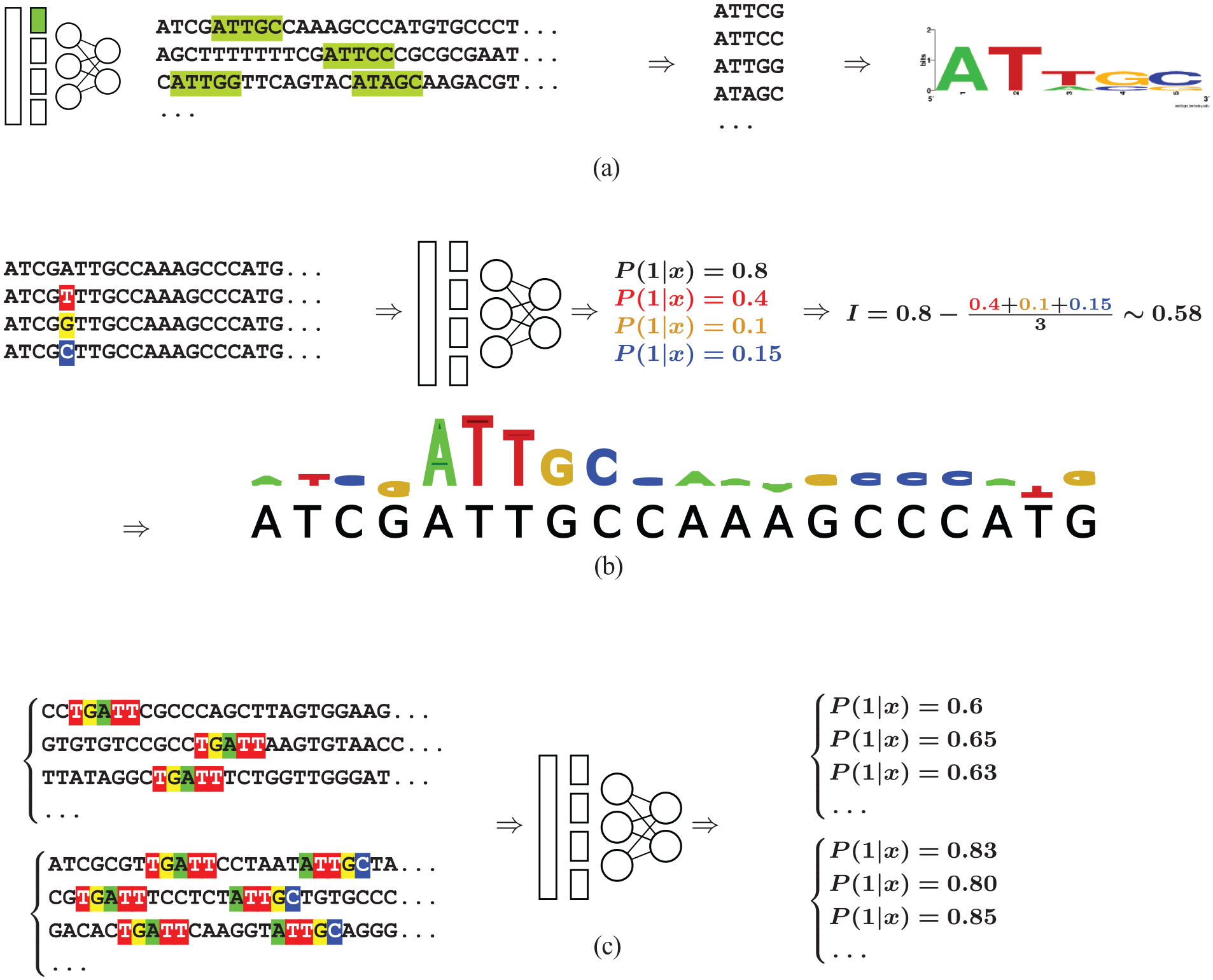
Three approaches for the interpretation of CNNs. (A) Explaining model components. The aim is to identify the motif encoded by each filter of the CNN (the figure illustrates the case for the first filter, in green). A set of sequences (e.g., the training sequences) are presented to the CNN and all sub-sequences that pass the activation threshold of the filter are identified (highlighted in green on the figure). The sub-sequences are then extracted and aligned (middle) and used to build a PWM logo (right) representing the motif encoded by the filter. (B) Explaining model predictions. The aim is to estimate the importance of each nucleotide of a target sequence (top left). The output value of the sequence is computed. In the example, the CNN computes a probability of binding, and the output value of the target sequence is P (1|x) = 0.8. For each nucleotide of the target sequence all possible mutations of that nucleotide are simulated in silico and output values are recomputed (the figure illustrates the case of the nucleotide A at position 5). The difference between the output of the original sequence and of all sequences with a different nucleotide at this position measures the importance of that nucleotide. The procedure is repeated at each position to estimate the importance associated with each nucleotide of the target sequence, which is represented by the height of the letters (bottom). Note that some nucleotides may have negative values if the mutations tend to increase the output value. (C) Exploring model behavior on synthetic sequences. Two sets of synthetic sequences are generated, and the output value of the CNN is computed for each sequence. In the example, all sequences embed a TGATT motif. In addition, the sequences in the second set also have an ATTGC motif located 6 nucleotides on the right of the TGATT motif. The difference in output between sequences from the first and second set thus measures the importance of motif ATTGC when used in combination with motif TGATT. Note that the procedure could be repeated by generating additional sets of sequences with different numbers of nucleotides between the 2 motifs, to investigate the importance of the distance between these motifs.

Explaining model predictions

Because of the partial motif problem, directly explaining a CNN remains a difficult question. Hence, several methods have been proposed to explain the predictions of the model rather than directly explaining the model. This involves using the model on a specific sequence and identifying the nucleotides that have the highest weight for the computation of the predicted value. The simplest method (known as input perturbation or in silico mutagenesis) is similar to the mutation maps proposed for variant identifications. It involves systematically simulating every single-nucleotide perturbation of the input sequence, and recording the effect induced on the predicted value^14,15,53 (see Figure 4B). Computing model prediction on every variant that can be obtained from single-nucleotide perturbations of a sequence may, however, induce high computational cost, specifically if the sequence is long, or if the analysis is repeated over many sequences. Backpropagation-based approaches have been proposed as more computationally efficient alternatives. The idea is to propagate an important signal from the output neurons to the inputs through the different layers of the model using a backpropagation algorithm. In this way, a single pass is sufficient to compute the contribution of each nucleotide to the output value. These contributions can then be visualized using saliency maps (see Figure 4B). Several approaches have been proposed on this idea (e.g., references.^66-68). In Zheng et al., ⁵³ a simulation-based study is used to benchmark these different approaches in the context of regulatory genomics.

By looking at the contribution scores of each nucleotide, one can identify the sub-sequences and regions that appear to be the most important for the prediction. Moreover, these sub-sequences can be further compared with known motifs to identify potential TFs involved in the regulation of the predicted signal. Hence, these approaches may highlight potentially interesting genomic information hidden into a specific sequence. However, it is important to note that because contribution scores are computed independently for each nucleotide, there is no warranty that the most important regions identified this way are really the most important regions for CNN prediction. Moreover, this analysis is restricted to the input sequence and is not sufficient to understand the general mechanisms used by the cell to regulate gene expression at different loci. For this, further analyses are needed. A possible approach is to compute the contribution of every nucleotide of all positive sequences and to extract the recurrent DNA motifs from these contribution maps. A first method is to use these maps to compute the average importance of every k-mer of a fixed length. The most important k-mers are then identified and compared with known TF motifs using approaches like TOMTOM. ⁶⁵ This is, for example the approach used in Zheng et al. ⁵³ to identify several co-factors that likely explain the binding differences between positive and negative sequences of 38 TFs. Another more sophisticated approach is to directly learn DNA motifs (using PWMs or close models) from the contribution maps. This is the aim of the TF-MoDISco method that segments the contribution maps into seqlets (a kind of weighted k-mers) and then clusters the seqlets in different motifs. ⁶⁹ This approach has been used in Avsec et al. ⁴² to identify core motifs and potential co-factors in 4 ChIP-seq experiments.

Thus, different approaches based on prediction explanation can also be used to identify motifs that are likely encoded into the structure of the CNN. However, in our opinion, an important difference with approaches based on the analysis of model components is that these methods lack an objective measure of importance associated with each motif. Indeed, it is not possible to turn the discovered motifs off in the CNN, and thus we cannot measure the accuracy of the model with and without a motif. Another problem is that there is no warranty that all important motifs used by the CNN were identified by the extraction procedure. Actually, it is even possible that some regulatory elements learned by the CNN but which were not identified by the motif extraction approach—eg, because these elements do not fit the kind of motifs searched by the extraction procedure—are actually more important for model predictions than the identified motifs.

Exploring model behavior on synthetic sequences

In the above sections, we have seen methods to extract some of the motifs that have been learned by a CNN for predicting a given signal. However, these interpretation methods are limited to the identification of simple motifs and cannot handle more sophisticated DNA features, such as the number of repetitions of a motif, the combination of several motifs, or their relative position on the sequence. For this, other approaches based on synthetic sequences have been proposed.

The first approach for this was the DeMo dashboard, ⁶⁷ which was inspired by the work of Simonyan et al. ⁶⁶ to interpret CNNs in the context of image recognition. DeMo aimed to predict TF binding with a CNN. To identify the genomic features captured by the CNN, the authors proposed to construct the best synthetic sequence that would maximize the binding probability according to the CNN. The idea was to provide the users with an archetype of the sequences with the highest binding probability, which supposedly bears the DNA features required for the binding. The idea was interesting but may miss certain features, especially if several (exclusive) rules govern the binding.

To go one step forward, Koo et al. ⁷⁰ proposed an approach named global importance analysis that samples a large number of synthetic sequences with and without a specific DNA feature and uses the learned CNN as an oracle to predict the binding associated with each sequence. If the predicted binding signal is statistically higher for the sequences that embed the studied DNA feature than for the others, the feature is considered important (see Figure 4C). The approach is interesting in that it can be used to assess any feature. For example, Koo et al. ⁷⁰ used it to show that increasing the number of repeats of the RBFOX1 motif increases the binding probability of the sequence according to their model. Similarly, they also showed that including some GC bias in sequence 3’ end also increases this probability. The approach was also used in Avsec et al. ⁴² to study the sinusoidal pattern that seems to regulate the distribution of the binding sites of the Nanog TF and its co-factors along the DNA sequence. It is important to understand that this approach is not a fully automatic method that would extract all DNA features captured by a CNN. Rather, specific hypotheses have to be constructed before being assessed by generating appropriate synthetic sequences. In this sense, the approach is similar to that of the ML models that directly take meaningful DNA features in input: In both cases, one can discover solely what has been formerly hypothesized.

One drawback of this importance measure is that it can sometimes lead to incorrect conclusions if the feature being tested is correlated with the functional element (e.g., if we test the hypothetical motif ATGCCA, while the true motif is actually GCCAA). Another drawback is that it is somewhat subjective, as it is only dictated by the model, with no link to its accuracy. The main issue is that the approach does not comply with a fundamental assumption in ML, which states that the training and test sets must be representative of the samples to classify. Here, the synthetic sequences do not follow exactly the same distribution as the sequences used to train the model and to estimate its accuracy. As a result, this accuracy may be an optimistic estimate of the accuracy of the model on the synthetic data. In other words, even if the model is quite good on the test sequences, it may be inaccurate on the synthetic sequences. This is related to the notions of extrapolation vs interpolation. Although ML models can be good at predicting a signal associated with a sequence that is close to other sequences in the training set (interpolation problem), when the sequence is far from any example of the training set (as the synthetic sequences can be) the problem is obviously more difficult, even if CNNs seem to be able to handle a certain level of extrapolation. ⁷¹ Note that the approach can nonetheless propose interesting hypotheses, which then need to be validated experimentally; however, users/experimentalists should be aware that the probability that these hypotheses hold can be lower than the model accuracy may lead one to believe.

Conclusions

Over the past decade, several ML models have been applied to the modeling of long regulatory sequences and have led to substantial advances in our understanding of regulatory genomics. These studies take place in a supervised framework, which enables, among other advantages, a fair comparison of model performance in terms of accuracy. From this perspective, deep learning approaches based on CNNs often show substantial improvement over simpler methods. This is especially true for the prediction of gene expression signal, where many efforts have been made to allow CNNs to handle very long sequences to capture the effect of potential distant enhancers, although this remains a difficult task. ¹⁸ Furthermore, it is important to keep in mind that although these approaches show impressive results for predicting gene expression levels across genes, their ability to explain expression variation between individuals is more limited.^19,20

Besides model accuracy, we have seen that different levels of knowledge can be gained by these studies. The prioritization of nucleotide variants, which is of great interest in medical and therapeutic studies, can be deduced from model predictions without the need for sophisticated procedures of model interpretation. Similarly, general hypotheses about the specificity or the extent of a regulatory mechanism can often be tested by training and swapping different models, or by changing the training or the test sets. On the contrary, identifying complex DNA features requires knowledge-extraction procedures that must be specifically adapted to the model at hand. The task is obviously easier for ML models that directly take these features in input than for CNN-based models that learn the predictive features from raw sequences. However, it would be inaccurate to consider these latter as complete black boxes, as several approaches are now available to extract such information. Notably, the oracle approach based on synthetic sequences looks like a promising avenue, ⁷⁰ provided that the generated sequences remain close to the training sequences to avoid misleading conclusions. Actually, in our opinion, the main limitation of CNN models lies in the difficulty to globally and objectively assess the importance of the extracted features. A related issue is the fact that we do not know with precision whether all important features have been extracted or if the CNN actually uses additional important features that were not identified. ⁵⁹

We have presented in this review some approaches for identifying the DNA features used by a specific model to make its predictions. A question that is rarely addressed in these studies is the stability of the model. DNA features are often highly correlated. For example, motifs of TFs of the same family are often very close. Moreover, motifs of co-factors often appear together at the same loci. Similarly, certain motifs are strongly enriched in DNA sequences with specific nucleotide or dinucleotide content. These strong correlations induce that different models with different DNA features may have close accuracy. As a result, the model that has been learned is not necessarily the only “good” model, a problem sometimes referred to as the Rashomon effect in ML (after the 1950 Japanese movie directed by Akira Kurosawa).^72,73 From this perspective, by aggregating the predictions of many models, ensemble ML approaches—and hence RFs—are less prone to this issue. ⁷² For other methods, analysis of model stability^74-76 or computing Shapley values ⁷⁷ can help. However, this requires repeating the learning procedure several times using slightly different learning sets, which can involve prohibitive computing time for very complex models.