Sage Journals: Discover world-class research

Abstract

We present a novel machine learning approach for the classification of cancer samples using expression data. We refer to the method as “decision trunks,” since it is loosely based on decision trees, but contains several modifications designed to achieve an algorithm that: (1) produces smaller and more easily interpretable classifiers than decision trees; (2) is more robust in varying application scenarios; and (3) achieves higher classification accuracy. The decision trunk algorithm has been implemented and tested on 26 classification tasks, covering a wide range of cancer forms, experimental methods, and classification scenarios. This comprehensive evaluation indicates that the proposed algorithm performs at least as well as the current state of the art algorithms in terms of accuracy, while producing classifiers that include on average only 2–3 markers. We suggest that the resulting decision trunks have clear advantages over other classifiers due to their transparency, interpretability, and their correspondence with human decision-making and clinical testing practices.

Keywords

classification machine learning gene expression biomarkers

Introduction

Numerous studies have been conducted to investigate if high-throughput gene and microRNA (miRNA) expression datasets can be used to differentiate between normal and tumor tissue, between tumors from different cancer forms, tumors in different stages, different responses to therapy, and so on. The earliest studies (eg, by Alon et al¹ and Golub et al)² focused on the use of unsupervised clustering analysis, whereas subsequent work exhaustively evaluated the usefulness of supervised classification approaches using standard machine learning methods.^3–8 A challenge in this scenario is to produce a classifier that is accurate and robust, while at the same time being interpretable, transparent, and able to provide some biological insight into the classification process.

Machine learning methods that have been applied to transcriptome data include “black box” methods such as support vector machines (SVM)^3,4,8 and artificial neural networks (ANN),^9–11 as well as symbolic and rule-based methods, such as decision trees.^11–13 The black box methods are statistically powerful and often provide good classification accuracy, but suffer from the drawback of producing non-transparent classifiers, which offer little or no insight into the basis for the classifications. In addition, these methods rely on using the complete marker set, or a large subset thereof. Decision tree methods, on the other hand, provide transparent and easily interpretable classifiers based on a relatively small set of markers, but suffer from the drawbacks of over-fitting, sensitivity to noise, and poor generality. Consequently, decision tree algorithms such as J48 and C4.5 have been among the worst performers in several comparisons of machine learning classification algorithms across different sets of cancer-related expression data.^14–17 The weaknesses of the decision tree approach can be counteracted by using random forests;¹⁸ however, this has the drawback of introducing complexity and producing models where the classification process is so non-transparent that it is essentially a black-box classifier.

A few algorithms have been proposed in efforts to overcome these challenges. A notable example is the top-scoring pairs (TSP) algorithm, which was introduced by Geman et al.¹⁵ The central idea of the TSP algorithm is to identify pairs of markers showing contrasting expression levels. If marker i is more highly expressed than marker j in most samples in one group (eg, cancer), while the opposite relation (ie, j being more highly expressed than i) holds for most samples in the second group (eg, normal), then the ij marker pair is a candidate for selection by the TSP algorithm. This seemingly simple approach has been shown to produce surprisingly powerful classifiers, with classification accuracy comparable to that of more complex methods, such as prediction analysis of microarrays (PAM)¹⁹ or SVM. Apart from the interpretability gained from using only two genes with a simple relationship, an additional advantage is that the classifier is independent of the actual expression levels, as long as the relation between the markers (one being lower or higher expressed than the other) is preserved. This makes the classifier less sensitive to experimental noise and facilitates the use of data from different labs, different experimental platforms, and so on.

An extended variant of TSP, called k-TSP, has been proposed,¹⁶ which identifies a set of k markers, where each pair casts a “vote” for one of the classes. Subsequently, classification is done by unweighted majority voting. This extended algorithm was shown to slightly improve the average classification accuracy, while preserving the property of the classifiers being simple and interpretable, given that k was limited to the range 1–10, corresponding to a maximum of 20 markers. A drawback, however, is that k-TSP classifiers do not show any particular relationship between the k marker pairs, since they all have equal amounts of influence on the classification. This is in contrast to a decision tree, where the root node contains the most important marker which identifies the major subclasses, while the markers further down the tree perform the finer “sorting” of samples within subclasses. Such a tree structure is attractive from a clinical perspective, since it reflects the human decision-making process (ie, first looking at the most important marker to make a tentative decision, and then at the less influential markers to fine-tune the decision) as well as the biology of the disease (ie, that some genes/miRNAs are highly influential and over-/underexpressed in most tumors, while other genes/miRNAs correspond to subclasses or special cases).

Other approaches have been proposed to reduce the number of markers used for classification and/ or to make the classifier more interpretable. Lauss and colleagues proposed a method that uses the receiver operating characteristic (ROC) to choose a small subset of genes and then builds a classifier on “metagenes,” which are expression profiles corresponding to the average expression values of the chosen genes across the set of probes.²⁰ Another variation on the top-scoring pairs theme has also been proposed where doublets were formed by different functions, such as the vector sum or difference between expression vectors of gene pairs.¹⁷ These doublets were then used as input into five standard classification methods, including SVM and decision trees, and improved accuracy was observed in comparison to the standard approach of using expression values of individual genes as input.

Herein we present a new classification algorithm, called the Decision Trunk Classifier, which has many features in common with decision trees, but with adaptations designed to make the algorithm more suitable for building classifiers for transcriptome data in clinical application scenarios. The goal of these adaptations is to gain classifiers that are smaller, simpler, and easier to interpret than standard decision trees, while at the same time achieving higher classification accuracy. An additional goal is to have a minimum number of parameters, since this will facilitate algorithm use, and should make it possible to avoid the over-fitting and inflated estimates of performance which may result from evaluating many combinations of parameter settings.

The key idea behind decision trunks is that for each internal node (marker) added to the “trunk,” all remaining samples are divided into three groups, for example a set of samples where the marker gene has: (1) high expression, (2) low expression, and (3) medium expression. To this node, three outgoing branches and nodes are then added, with one corresponding to each group, and with the “low” and “high” nodes being leaf nodes where a decision is made according to the majority class of the group. The third, “middle” node corresponds to uncertain cases and is therefore an internal node where no decision is made. Instead, a new marker is chosen for this node, and the reduced set of samples is again divided into those with low, high, and intermediate expression levels for this marker. This process continues until a stopping criterion is reached and a final marker is chosen. The node for this marker has only two outgoing branches (for low and high expression), both leading to leaf nodes. The result of this process is a “slim” decision tree, consisting only of a straight “trunk” with decision nodes pointing out from the trunk.

We hypothesize that the use of a medium expression level interval for uncertain cases, and deferring the decision to the next level of the trunk, will result in higher robustness to noise than in standard decision trees. We also claim that decision trunks will be easier to interpret and relate to the underlying biology, as well as to clinical testing practices, than standard decision trees. The proposed method has been implemented and tested on a large number of expression datasets, and its classification accuracy has been compared to a wide variety of other methods, including both standard machine learning algorithms and special-purpose algorithms designed for expression data.

Methods

Algorithm Overview

As input, the decision trunk classifier requires a dataset consisting of expression values for N probes {p₁, …, p_N}, which represent genes or miRNAs, and M tissue samples {x₁, …, x_M}. The entire dataset is stored in a N × M dimensional matrix, where e_ij denotes the expression value of the i-th probe i ∈ {1, …, N} for the j-th tissue sample j ∈ {1, …, M}. The class labels for the tissue samples are represented by a vector y = {y₁, …, y_M} where y_j ∈ {C₁, …, C_k} is a set of k class labels. All classification problems discussed in this paper are binary (k = 2).

Usage of the algorithm can be divided into three steps: (1) building decision trunks; (2) choosing the number of decision levels; and (3) evaluating classification accuracy. During the first step, five sets of decision trunks are built with L = 1, …, 5 decision levels. Each set consists of M decision trunks, where each decision trunk is generated with a different training set of M-1 samples as input. The purpose of these sets of classifiers is to do a stability analysis, by gathering statistics on how much the choice of markers varies between decision trunks in each set. The second step consists of choosing the number of levels for the output classifiers based on the results of the stability analysis. In the third step, either leave-one-out cross validation (LOOCV) or a split-sample procedure is applied to evaluate the classification accuracy. This evaluation is conducted only on the decision trunks with the chosen number of levels.

Building Decision Trunks

To build a decision trunk, the algorithm first creates a decision trunk object and then adds to it one decision level at a time. For every level, a t-score is computed for each probe, given the division of the N expression values for each probe into two classes. The t-score is calculated as:

t = \frac{| {\bar{X}}_{C_{1}} - {\bar{X}}_{C_{2}} |}{\sqrt{\frac{σ_{C_{1}}^{2}}{N_{C_{1}}} + \frac{σ_{C_{2}}^{2}}{N_{C_{2}}}}}

(1)

where ${\bar{X}}_{C_{i}}$ is the mean and $σ_{C_{i}}^{2}$ is the variance of the expression values of the given probe in class i, while N_Ci represents the number of samples in class i. The probe with the highest t-value is chosen as the decision node. Let this probe be represented by index k ∈ {1, …, N}. The samples are then ranked according to their expression values e_kj, j = {1, …, M} (ie, according to their expression levels for the chosen probe) (see left panel in Fig. 1). The class label of the sample with lowest expression is set as C_low and the opposite class label is stored as C_high. Next, the class label of every sample is compared to C_low, starting at the sample with the lowest expression and proceeding until the first C_high sample is found, or until one quarter of all samples have been checked (whichever comes first). A lower decision threshold, T_low, is then calculated as the average expression of the last seen C_low sample and the first C_high sample. The procedure is then repeated starting at the sample with the highest expression and proceeding until the first C_low sample is found or until one quarter of all samples have been checked. An upper decision threshold, T_high, is then calculated as the average of the last seen C_high sample and the first C_low sample.

Figure 1.

Left panel: A number of malignant and normal samples are ranked according to their expression values for the marker with the highest t-value. The upper and lower thresholds (indicated by dashed lines) are determined as described in the text. Right panel: The decision node d₁ has two thresholds (T_low and T_high) for the expression value e, which are used for classifying samples as normal or malignant, respectively. For decision node d₂ only the remaining samples, with intermediate expression of the d₁ marker, will be used for selection of a new marker, according to recalculated t-values.

When the decision thresholds have been set, the algorithm removes all samples whose expression values are lower than T_low or higher than T_high. Following this, the algorithm continues to add another level to the decision trunk by using the remaining samples to select a new probe. This is repeated until the last level is reached. Since the last level should only have one decision threshold, this is calculated as the average of T_low and T_high.

Figure 1 illustrates the process of generating decision nodes. The samples are ranked according to their expression values for the most significant marker and the upper and lower thresholds for expression value e are determined. Three edges extend from the decision node, two of which lead directly to classifications, whereas the third (middle) one will defer the decision until later. Thus, any sample with a distinctly low or high expression value for the chosen marker will immediately be classified as “normal” or “malignant,” respectively, whereas any sample with an intermediate expression value for this marker will be tested with the next marker (decision node d₂). When choosing the marker for d₂, only the remaining ≥ 50% of samples will be included in the calculation of t-values, the ranking of candidate markers and samples, and in the selection of expression thresholds. This means that decision nodes further down the tree can be based on genes/miRNAs where differential expression is observed only for a subset of tumors and which may be characteristic for subtypes of the given tumor type.

Choosing the Number of Decision Levels

To choose the number of decision levels, the algorithm checks how many features are selected at each level when decision trunks are built from the M training sets. The purpose of this is to measure the stability of feature selection at each of the five levels, L = 1, …, 5. Stability is defined as follows: during the M training rounds, for a given level of the decision trunk, a maximum of six different features are selected. When the highest value of L that fulfills the stability criterion has been determined, decision trunks with this number of levels are presented as output of the algorithm. If no level is found to fulfill the stability criterion, decision trunks with a single level are used instead. It should be noted that no evaluation of classification accuracy is done in this procedure, meaning that the choice of L is based solely on the stability criterion. The evaluation of classification accuracy follows as the next and final step, and is performed only on decision trunks with the chosen number of levels.

Feature Selection

In addition to the t-score (described in section “Building decision trunks”), we also implemented and tested a feature selection method based on calculating a polarization score for each feature in the dataset and selecting the feature with the highest score. The polarization score Pscore_i of a feature i is determined by first ranking all samples in ascending order according to their expression values for the feature. The class label of the sample with the lowest expression is set as C_low and the opposite class label is stored as C_high. Next, the class label of each sample is checked starting at the sample with lowest expression. For each sample with the C_low class label, the counter for the size of |P_low| is incremented by one. This continues until a sample of the opposite class is encountered. The procedure is then repeated in the opposite direction, starting at the sample with highest expression, to calculate the size of |P_high|. Finally, Pscore_i is calculated as:

P s c o r e_{i} = \frac{| P_{l o w} | + | P_{h i g h} |}{2}

We refer to this method as maximum class polarization (MCP), as it selects the feature that results in the most polarized division of the samples into two groups. Similar feature selection methods have been suggested and tested by Park et al²¹ and Dettling and Bühlmann,¹² and these methods can be considered as adaptations of the Wilcoxon test statistic.

Implementation

The main part of the decision trunk algorithm was implemented in Perl. For efficiency reasons, the feature selection methods were implemented as a shared C library. The program is executed from the command line and requires a text file containing an expression data table as input. The table must have column names on the first row and row names in the first column. Furthermore, the user is expected to supply the name of the classification variable to be used. Class information is supplied as metadata (rows starting with “#”) at the top of the file. To facilitate the generation of the metadata, the program also accepts a supplementary file with the -s argument. This file should have a header, followed by any number of rows. These rows start with a sample name, followed by columns containing class labels. In the header of these columns, the names of the class variables should be given. More details on the usage of the software are supplied in the online documentation. The implementation of the algorithm is available as the Algorithm::TrunkClassifier package at CPAN.

As output, the program reports: (1) the accuracy for each round of evaluation (LOOCV or split-sample), as well as the overall average accuracy; (2) the decision trunk classifiers generated during the evaluation; (3) to which class and at what level in the decision trunk each sample was classified; (4) a log file containing the parameters used and sizes (number of samples) of the two classes.

Datasets and Evaluation Methods

The datasets used in this study contain expression data for a set of features (genes, miRNAs or NGS reads) from 13 published studies covering cancers of the prostate, bladder, breast, and lung, as well as neuroblastomas. The majority of studies were used for more than one classification task. For example both normal versus malignant and early versus late stage were used for the Sanchez bladder cancer data. Thereby, a total of 26 different classification tasks were formulated. A summary of the datasets and classification variables is given in Table 1. For bladder cancer datasets, the early stage was defined as Ta/T1, and late stage as ≥ T2. For breast cancer datasets, histologic grade 1 was considered as low grade and histologic grade > 1 as high grade. For neuroblastoma datasets, the International Neuroblastoma Staging System (INSS) stage 1–2 was defined as early stage and INSS stage > 2 as late stage. The Sanchez, Stransky, WangY, Sotiriou and Janoueix datasets were log2-transformed before classification. All datasets were examined for missing values and genes with >5% missing values were removed. The remaining missing values were imputed by taking the average of all values for that gene.

Table 1.

Description of datasets and classification variables.

Dataset¹	Cancer	Class 1	Class 2	Samples	Probes	Acc. no.	Ref.
Carlsson1	Prostate	Normal	Malignant	38	768		41
Carlsson2	Prostate	Normal	Malignant	76	664		42
Singh	Prostate	Normal	Malignant	101	12533		30
Sanchez_NM	Bladder	Normal	Malignant	129	22283		31
Sanchez_ST	Bladder	Early stage	Late stage	91	22283		31
Sanchez_GR	Bladder	Low grade	High grade	91	22283		31
Sanchez_SU	Bladder	Alive	Dead	91	22283		31
Stransky_ST	Bladder	Early stage	Late stage	57	12599	E-TABM-147	32
Stransky_GR	Bladder	Low grade	High grade	55	12599	E-TABM-147	32
VandeVijver_ER	Breast	ER+	ER–	295	13359		33
VandeVijver_SU	Breast	Alive	Dead	295	13359		33
WangY	Breast	ER+	ER-	286	22283	GSE2034	34
Sotiriou_TR	Breast	Tamoxifen	Untreated	189	22283	GSE2990	35
Sotiriou_GR	Breast	Low grade	high grade	167	22283	GSE2990	35
Sotiriou_ER	Breast	ER+	ER-	183	22283	GSE2990	35
WangQ_ST	Neurobl.	early stage	Late stage	101	12625	GSE3960	36
WangQ_MY	Neurobl.	MYC–	MYC+	101	12625	GSE3960	36
Janoueix_ST	Neurobl.	Early stage	Late stage	64	54613	GSE12460	37
Janoueix_MY	Neurobl.	MYC–	MYC+	45	54613	GSE12460	37
Attiyeh_ST	Neurobl.	Early stage	Late stage	100	48701	GSE19274	38
Attiyeh_MY	Neurobl.	MYC–	MYC+	134	48701	GSE19274	38
Angulo_HI	Lung	Adenocarc.	Squam.	66	20185	GSE8569	39
Angulo_DI	Lung	Well diff.	Poorly diff.	51	20185	GSE8569	39
Takeuchi_HI	Lung	Adenocarc.	Squam.	125	21619	GSE11969	40
Takeuchi_DI	Lung	Well diff.	Poorly diff.	59	21619	GSE11969	40
Takeuchi_SU	Lung	Alive	Dead	149	21619	GSE11969	40

NM, normal versus malignant; ST, stage; TR, treatment status; GR, grade; ER, estrogen receptor status; M Y, MYC amplification status; HI, histological subtype; DI, differentiation status; SU, survival.

The evaluation of classification accuracy was performed using LOOCV with the number of folds equal to the number of samples. The average accuracy for the given dataset was defined as the proportion of correctly classified test samples (which is equivalent to the number of true positives plus the number of true negatives divided by the total number of samples). The performance of the decision trunk algorithm was compared with that of the following algorithms: Naïve Bayes (NB), Decision Trees (J48), Voting Features Interval (VFI), SVM, single layer Artificial Neural Network (ANN), k-Nearest Neighbor (kNN), Prediction Analysis for Microarrays (PAM), TSP, and the Metagene Classifier (ROCC). Weka version 3.6.6 was used for NB, J48, VFI, SVM, and ANN, whereas Bioconductor packages were used for kNN (ver. 7.3–1), PAM (ver. 1.54), TSP (version 2.8), and ROCC (version 1.2). All algorithms were run with default parameters except kNN and PAM. For kNN, the parameter k was set to 3, and for PAM the number of thresholds chosen was 1.

In addition to cross-validation, the decision trunk algorithm was further evaluated using three different approaches. The first approach consisted of a split-sample procedure, where each one of the 26 datasets was divided randomly ten times into a training set, containing 80% of the samples, and a test set containing the remaining samples. In the second approach 40 artificial datasets were generated using two random normal distributed variables, one for each class. Each dataset consisted of 200 samples per class, with the two classes having equal standard deviations but different means. The standard deviations were set to 0.5, 1.0, 1.5, 2.0 (four values) and the difference between the means was set to 0.5, 1.0, …, 5.0 (ten values). The third approach aimed to test the generality of the algorithm by using data from one study as the training set and data from another study as the test set. This was done using the Sanchez dataset for training and the Stransky data for testing, and vice versa. This combination of datasets was chosen since both studies were on bladder cancer and aimed to address the same classification problems, namely grade and stage.

Results

The decision trunks generated for the 26 datasets had on average 2.0 levels. To illustrate the argument that this gives transparent and easily interpretable classifiers, Figure 2 shows the decision trunk for the Carlsson1 dataset (quantitative polymerase chain reaction (qPCR) data on prostate cancer tumors versus healthy prostate tissue). Only two markers, miR-126* and miR-892b, are included in the classifier. Samples with very low qPCR values for miR-126* (<23.2) are assigned class N (normal) and samples with very high values for miR-126* (>25.28) are assigned class M (malignant). Samples with intermediate values for miR-126* are assigned a class based on their expression of miR-892b. LOOCV accuracy for this simple classifier was 97.36%. The accuracy of classifiers generated by the other algorithms on the same dataset ranged from 76.32% (SVM) to 94.47% (NB, J48, VFI, PAM, and TSP). The microRNA miR-126* has been identified in many studies as being associated with several cancer forms, including prostate cancer,^22,23 while miR-892b has not previously been recognized as deregulated in cancer.

Figure 2.

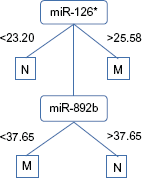
Example of decision trunk generated from the Carlsson1 dataset.

Classification accuracies on all datasets of the decision trunk classification algorithm (DTC), as well as all the algorithms evaluated for comparison, are presented in Table 2. A general trend is that the average performance of all algorithms is quite high. DTC had the highest average classification accuracy (84.47%) and was the best performing of all algorithms on 11 of the 26 datasets (42%). The second and third highest average classification accuracies were achieved by ROCC (83.71%) and kNN (81.34%), which where the best performing algorithms on five (19%) and one (4%) datasets, respectively. ANN also reached > 80% in average classification accuracy, while the remaining algorithms (NB, J48, VFI, SVM, PAM, and TSP) had average accuracies in the range 70% to 80%. It is noteworthy that three of the five best performing algorithms in this evaluation (DTC, ROCC, and TSP) have been designed for expression data, and have the goal of using a minimal number of markers. General-purpose classification algorithms, such as NB, J48, VFI, and SVM, as well as special purpose algorithms using a large set of markers (ie, PAM), generally gave poorer results.

Table 2.

Classification accuracies for all algorithms as determined by leave-one-out cross validation.

Dataset	DTC	J48	NB	VFI	SVM	ANN	KNN	PAM	TSP	ROCC
Carlsson1	97.36	94.74	94.74	94.74	76.32	84.21	86.84	94.74	94.74	89.47
Carlsson2	78.94	96.05	85.53	81.58	84.21	90.79	88.16	85.53	89.47	89.47
Singh	89.21	87.25	62.75	74.51	50.98	91.18	76.47	62.75	95.10	87.25
Sanchez_NM	91.47	87.60	89.92	83.72	93.03	92.25	91.47	88.37	91.47	91.47
Sanchez_ST	90.11	91.21	89.01	72.53	92.31	89.01	89.01	82.42	83.52	90.11
Sanchez_GR	87.91	59.34	83.52	29.67	80.22	83.52	84.62	73.63	87.91	84.62
Sanchez_SU	72.53	59.34	61.54	65.93	57.14	57.14	58.24	57.14	37.36	62.64
Stransky_ST	75.43	52.63	82.46	82.46	82.46	75.44	84.21	87.72	80.70	85.96
Stransky_GR	89.09	80.00	81.82	78.18	81.82	78.18	83.64	78.18	76.36	80.00
VandeVijver_ER	100.0	99.66	89.15	85.76	84.41	92.54	91.19	92.20	95.25	95.93
VandeVijver_SU	71.19	66.10	53.56	64.41	73.22	66.78	70.17	69.15	57.97	69.83
WangY	89.86	75.17	87.41	49.30	86.71	87.76	84.27	87.41	77.97	89.86
Sotiriou_TR	98.94	98.41	87.30	96.30	87.30	96.30	93.65	87.30	100.0	99.47
Sotiriou_GR	76.04	67.07	64.07	74.25	64.07	60.48	74.25	64.07	68.26	70.66
Sotiriou_ER	76.50	78.69	44.26	53.55	81.42	82.51	87.43	40.98	84.15	88.52
WangQ_ST	83.16	73.28	82.18	69.31	72.28	82.18	82.18	78.22	48.51	80.20
WangQ_MY	100.0	99.01	96.04	72.28	80.20	96.04	98.02	94.06	98.02	96.04
Janoueix_ST	65.63	59.38	67.19	68.75	65.63	65.63	71.88	70.31	84.38	73.44
Janoueix_MY	84.44	91.11	77.78	68.89	68.89	73.33	84.44	80.00	82.22	84.44
Attiyeh_ST	78.00	66.00	86.00	31.00	83.00	81.00	90.00	76.00	61.00	90.00
Attiyeh_MY	87.31	89.55	78.36	62.69	67.91	89.55	79.10	76.87	91.79	82.09
Angulo_HI	89.39	77.27	89.39	89.39	89.39	90.91	80.30	89.39	87.88	95.45
Angulo_DI	74.50	70.59	70.59	62.75	74.51	60.78	66.67	62.75	76.47	68.63
Takeuchi_HI	94.40	90.40	93.60	72.00	72.00	95.20	93.60	94.40	89.60	95.20
Takeuchi_DI	86.44	66.10	69.49	77.97	57.63	79.67	72.88	79.66	77.97	84.75
Takeuchi SU	68.45	41.61	53.02	55.70	27.52	41.61	51.68	55.03	56.38	51.01
Average	84.47	77.60	77.72	69.91	74.41	80.15	81.34	77.24	79.79	83.71

Note: Bold values indicate the best performing algorithm(s) for each dataset and the best average accuracy over all datasets.

Comparing the decision trunk classifier to the standard decision tree algorithm J48 reveals that DTC seems to do better on average by being more robust. The two algorithms show comparable performance for many datasets, but J48 occasionally fails and performs considerably worse. This occurred in particular on the datasets Sanchez_GR (87.91% versus 59.34%), Takeuchi_SU (68.45% versus 41.61%), Stransky_ST (75.43% versus 52.63%), and Takeuchi_DI (86.44% versus 66.10%). The higher robustness of DTC can also be seen in the standard deviations of the two algorithms' accuracies over all datasets, which are 9.6 and 16.0, respectively. A one-sided Student's t-test for paired values shows that the difference in average results between DTC and J48 (84.47% versus 77.60%) is significant at the P < 0.01 level (P = 0.0011). A striking difference between the decision trunks and decision trees is the number of markers (nodes) used in the classifiers. While the average number of nodes (levels) in the decision trunks was only 2.0, the average number of nodes in the J48 decision trees was 9.9. It is noteworthy that the “failed” decision trees mentioned above for the Sanchez_GR, Takeuchi_SU, Stransky_ST, and Takeuchi_DI datasets, had on average 13 decision nodes. There were four datasets, however, for which J48 produced very small decision trees with only three decision nodes. In all four of these cases, the classification accuracy was on par with that of the DTC algorithm (Carlsson1: 97.36% for DTC versus 94.74% for J48; VandeVijver_ER: 100% versus 99.66%; Soutirou_TR: 98.94% versus 98.41%; WangQ_MY: 100% versus 99.01%). Figure 3 shows the relationship between the number of nodes and classification accuracy for both algorithms. While there is a clear correspondence between decision tree size and decreased performance, no such trend can be observed for decision trunks.

Figure 3.

Relationship between classification accuracy and the number of decision nodes (markers) for J48 decision trees (red) and the decision trunk algorithm (black) on the 26 datasets.

The accuracies for the DTC reported in Table 2 were obtained when using the stability criterion (see Methods) for selection of the number of levels (L). To investigate if this method for selecting L performs well or if there is substantial room for potential improvement, we compared its results with those gained when choosing the L that gives optimal results (Table 3). It was found that choosing L based on the stability criterion gave less than optimal results on only nine of the 26 datasets (35%), and that the difference in average classification accuracy was around two percentage points (84.47% versus 86.33%). The method based on stability criteria can be described as being slightly conservative, in the sense that it usually fails by building decision trunks that are too small (in six out of nine cases). The average L for the method based on stability criteria was 2.04, as compared to 2.08 when choosing the L that gives the best classification results.

Table 3.

Decision trunk accuracies achieved using a posteriori selection of optimal number of levels (left) and using stability criteria (right).

Dataset	Optimal		Stability
Dataset	L	Accuracy	L	Accuracy
Carlsson1	2	97.36	2	97.36
Carlsson2	3	86.84	2	78.94
Singh	4	90.19	3	89.21
Sanchez_NM	2	91.47	2	91.47
Sanchez_ST	3	90.10	3	90.10
Sanchez_GR	1	87.91	1	87.91
Stransky_ST	1	80.70	2	75.43
Sanchez_SU	2	72.53	2	72.53
Stransky_GR	2	89.09	2	89.09
VandeVijver	1	100.0	1	100.0
VandeVijver_SU	2	79.32	5	71.19
WangY	5	89.86	5	89.86
Sotiriou_TR	2	98.94	2	98.94
Sotiriou_GR	2	76.04	2	76.04
Sotiriou_ER	3	89.07	2	76.50
WangQ_ST	2	83.16	2	83.16
WangQ_MY	1	100.0	1	100.0
Janoueix_ST	2	68.75	1	65.62
Janoueix_MY	2	86.66	1	84.44
Attiyeh_ST	3	83.00	1	78.00
Attiyeh_MY	1	87.31	1	87.31
Angulo_HI	1	89.39	1	89.39
Angulo_DI	1	74.50	1	74.50
Takeuchi_HI	1	97.60	3	94.40
Takeuchi_DI	1	86.44	1	86.44
Takeuchi_SU	4	68.45	4	68.45
Average	2.08	86.33	2.04	84.47

Notes: The nine cases where results differ are marked in bold. In six of the nine cases, the stability criterion leads to non-optimal results by choosing a lower L. The difference in average accuracy was less than two percentage points.

The split-sample approach was applied to further evaluate the robustness of the DTC algorithm. Each of the 26 datasets was repeatedly split into training and test sets and the average classification accuracy recorded (Supplementary Table 1). The resulting average accuracy sank to 79.17%. Thus, after this moderate drop of just over five percentage points, the average accuracy of the DTC was still above the performance of J48 and four other algorithms in the cross-validation (compare with Table 2).

The difficulty of a classification task depends on the distributions of expression values for the two classes to be separated. The greater the overlap between the distributions, the more difficult it will be to classify the samples correctly. To investigate this relationship between distribution and accuracy, 40 artificial datasets with a range of standard deviations and differences between means were generated. The average accuracies of decision trunks generated using these datasets are shown in Figure 4, along with the accuracies for the cancer datasets. Accuracies range from 80%–100% for artificial datasets with an SD = 0.5, regardless of the difference between means, while 1 ≤ SD ≤ 2 requires a difference between means of 1 to 2.5 to achieve 80% accuracy. For comparison, the accuracies from the 26 cancer classification tasks (Table 2) were also plotted in Figure 4. Considering the SD for the top-level marker in the trunks generated from these datasets, most of the classification accuracies are similar to those obtained from the artificial data. There are cases to the far right in the plot, where classification accuracy on cancer datasets is lower than expected. However, these datasets had very high SD (up to 9.6), which explains why accuracy is lower than on the artificial datasets where SD was limited to a maximum of 2.

Figure 4.

Decision trunk classification accuracies for artificial and cancer datasets.

As a test of generality, the DTC algorithm was applied using data from one study as the training set and data from another study as the test set. The two microarray gene expression datasets (Sanchez³¹ and Stransky)³² concern bladder cancer and contain a stratification of tumors according to grade and stage. The probe IDs in both datasets were converted to HUGO Gene Nomenclature Committee symbols, and genes unique to either dataset were removed. Normalization was carried out by dividing the expression values for each gene by the mean expression of the gene, for each dataset separately. Four classification tasks were then carried out, namely by training on Sanchez, and classifying Stransky (and vice versa), first for tumor grade and then for stage. Comparing the results with Table 2, it can be seen that there is essentially no loss of accuracy when classifying the Stransky grade data: 87.27% when training on the Sanchez data versus 89.09% when training on the Stransky data. When classifying the Stransky stage data, accuracy dropped to 66.67% when training on the Sanchez data, compared to 75.43% when training on the Stransky data. Loss of accuracy was generally greater when classifying samples from the Sanchez dataset: from 87.91% to 65.93% for grade and from 90.11% to 73.63% for stage. The greater loss in accuracy when training on the Stransky data can be explained by the fact that the Stransky dataset contains 55 (grade) and 57 (stage) samples, while the Sanchez dataset contains 91 samples for both grade and stage.

To further evaluate the usefulness of selected genes as cancer biomarkers, a comparison of selected markers was conducted between the DTC algorithm and J48. The idea is that if several different approaches identify a gene as a useful marker for classification, it is more likely to be robust. For DTC and J48, the root nodes were compared to determine the overlap of marker selection. Only in six of the 26 classification tasks did the algorithms choose the same marker for their top-level nodes, and this corresponds to the cases where both algorithms perform well.

Discussion

Comparison with other Decision Tree Variants

There are several variations on the theme of decision trees. A simplified version, named decision stumps, generates classifiers containing a single decision node with k outgoing branches, each leading to a leaf node representing one class.²⁴ Random forests consist of sets of decision trees which complement each other in the decision-making process and where the decision is made by summing up the votes of the individual trees.¹⁸ We here introduced a new variation on the decision tree theme, which we named decision trunks, since our classifiers consist of a single sequence of decision nodes, thus resembling the trunk of a tree.

Decision trunks bear some resemblance to fuzzy decision trees,²⁵ a method designed to address the problem that decision trees were originally designed for attributes that take on a discrete set of values. For continuous domains, such as expression data, the attributes must be discretized. This can be done by partitioning the attribute range into two intervals,²⁶ but the “crisp” cutting points resulting from standard decision trees produce high error rates in many real-world applications due to vague and noisy data.²⁷ Fuzzy decision trees were designed to overcome this problem by implementing a “soft” form of discretization.²⁵ A standard decision tree, using crisp discretization, partitions the decision space into a set of non-overlapping subspaces and assigns each object a particular class. In contrast, a fuzzy decision tree, using soft discretization, allows an object to be associated with different paths in the tree and assigns the object a probability of belonging to each class.²⁷ This has been shown to improve robustness in many applications, but at the cost of a more complex training procedure, the introduction of parameters, and trees that are not as easy to interpret as standard decision trees. Decision trunks offer a third alternative, which can be seen as containing some elements of both approaches. The decision trunks algorithm sets crisp thresholds, but only to identify those samples that are clearly defined by a given probe, while deferring decisions on the remaining samples to the next lower level in the trunk. The results presented in this paper indicate that this improves generality and robustness, while giving classifiers that are even simpler and easier to interpret than standard decision trees.

The limited performance of standard decision trees on expression data has also been addressed by using boosting.^3,7,12 The improved classification accuracy of such approaches comes with drawbacks such as the introduction of additional parameters (eg, the number of boosting iterations), and an increased computational cost.

Alternative Methods for Feature Selection

The standard method for feature selection in decision tree algorithms is information gain. Information gain is based on the entropy function, i_t = – p_t log(p_t) – (1 – p_t) log(1 – p_t), where p_t is the proportion of samples in node t that belong to a given class (in a binary classification problem). Thus, i_t measures the “impurity” of node t and is maximal in the root node, where half of the samples belong to each class, and minimal in leaf nodes where all samples belong only to one class. When selecting a marker and expression threshold for the root node t = 1, we will effectively divide the sample set into two subsets, represented by two daughter nodes t = 2 and t = 3. When doing so, we want to minimize the weighted impurity, i₂r₂ + i₃r₃, where r_i is the proportion of samples in node i. Standard decision tree algorithms, therefore, select the combination of marker and expression threshold that maximizes this reduction in impurity (ie, gain in information) for each new node added to the tree.

In order to facilitate comparisons with standard decision tree algorithms, we would want to use the information gain criterion for the selection of markers in decision trunks. This would give a clearer idea of what feature(s) of the decision trunks algorithm that the gains in classification accuracy can be attributed to. Unfortunately, the information gain criterion cannot be implemented in decision trunks without modifications. The decision trunks algorithm adds three outgoing branches from each decision node (in a binary classification problem), and the daughter nodes have different interpretations. The two leaf nodes are, by definition, maximally pure and the middle node is, by definition, impure. Since the upper and lower decision thresholds are calibrated by the quartiles of the sample set, the reduction in impurity (ie, information gain) is constrained in such a way that a huge number of marker and threshold combinations would achieve the same information gain. Thus, information gain is not a meaningful marker selection criterion for classifiers of this type.

Further Development

An attractive feature of decision trees, which also applies to decision trunks, is that a set of symbolic rules can be derived from a decision tree and implemented in a rule-based decision system.¹⁴ The decision nodes on the path leading to the leaf node generate a conjunctive antecedent and the classification specified by the leaf generates the consequent of an “if-then” rule on the form if [e₁< θ₁]Λ … Λ[e_i < θ_i] then C_j, where θ_i represents a threshold value of expression for probe i. Thus, a further development could be to use the decision trunks algorithm to generate rule-based decision support systems.

It can be advantageous in some application scenarios to be able to build classifiers with the option to assign the class label “uncertain” to some samples.¹² This could easily be achieved by a slight modification of the decision trunks algorithm, by simply letting the bottom-level node of the decision trunk have three outgoing branches, labeled C₁, C₂, and “uncertain.” Thus, the last node in the decision trunk would be built in the same way as the internal nodes, with upper and lower thresholds based on the limits of the upper and lower quartiles, and the intermediate node representing uncertain samples. These would be presented to the user for manual inspection or classification using other algorithms.

The decision trunks algorithm is designed for binary classification problems. Multiclass problems can nevertheless be handled using the one-against-all approach, which is commonly used in the machine learning community.^28,29 It reduces a classification problem with k classes (k > 2) into k binary classification problems, where the class label for a given sample in the j th problem is 1 if C_j = j and, 0 otherwise. The whole process of training and testing decision trunks is then repeated for each binary problem, leading to the creation of j decision trunk classifiers, each being specialized on a given class. It would, in principle, be possible to extend the decision trunk algorithm to handle multi-class classification directly, although this would make the algorithm substantially more complicated.

Conclusions

The decision trunk algorithm provides classifiers that: (1) involve a minimal set of markers; (2) are as accurate as classifiers produced by the most powerful machine learning methods; and (3) are easily interpretable and correspond to clinical test procedures. In addition, the algorithm is essentially parameter-free since it is possible to use the stability criterion for setting the parameter L, and therefore also easy to use. Although more tests are certainly always needed, the quite comprehensive evaluation presented in this paper strongly indicates that the algorithm performs equally well as, if not better than, the current state of the art algorithms for the classification of cancer samples using expression data.

Author Contributions

Conceived the idea of a decision trunks algorithm: BO. Jointly developed algorithm details: BU, BO. Implemented the algorithm: BU. Jointly designed the evaluation experiments: BU, BO. Collected the datasets and carried out all experiments: BU. Jointly analyzed the results: BU, KKL, BO. Developed the structure and main arguments of the paper: BO. Made critical revisions and updates of the manuscript: BU, BO, KKL. All authors reviewed and approved of the final manuscript.

Funding

This work was partially funded by the Swedish Knowledge Foundation, (grant 2009/0291).

Competing Interests

Author(s) disclose no potential conficts of interest.

Disclosures and Ethics

As a requirement of the publication, author(s) have provided to the publisher signed confirmation of compliance with legal and ethical obligations including but not limited to the following: authorship and contributorship, conflicts of interest, privacy, and confidentiality, and (where applicable) protection of human and animal research subjects. The authors have read and confirmed their agreement with the ICMJE authorship and conflict of interest criteria. The authors have also confirmed that this article is unique and not under consideration or published in any other publication, and that they have permission from rights holders to reproduce any copyrighted material. Any disclosures are made in this section. The external blind peer reviewers report no conflicts of interest.

References

Alon

, Barkai

, Notterman

Broad patterns of gene expression revealed by clustering analysis of tumor and normal colon tissues probed by oligonucleotide arrays.

Proc Natl Acad Sci U S A. 1999; 96(12): 6745–50.

Golub

T.R.

, Slonim

D.K.

, Tamayo

Molecular classification of cancer: class discovery and class prediction by gene expression monitoring.

Science. 1999; 286(5439): 531–7.

Ben-Dor

, Bruhn

, Friedman

, Nachman

, Schummer

, Yakhini

Tissue classification with gene expression profiles.

J Comput Biol. 2000; 7(3-4): 559–83.

Furey

T.S.

, Christianini

, Duffy

, Bednarski

D.W.

, Schummer

, Haussler

Support vector machine classification and validation of cancer tissue samples using microarray expression data.

Bioinformatics. 2000; 16(10): 906–14.

West

, Blanchette

, Dressman

Predicting the clinical status of human breast cancer by using gene expression profiles.

Proc Natl Acad Sci U S A. 2001; 98(20): 11462–7.

Zhang

, Yu

C Y.

, Singer

, Xiong

Recursive partitioning for tumor classification with gene expression microarray.

Proc Natl Acad Sci U S A. 2001; 98(12): 6730–5.

Dudoit

, Fridlyand

, Speed

T.P.

Comparison of discrimination methods for the classification of tumours using expression data.

Journal of the American Statistical Association. 2002; 97: 77–87.

Guyon

, Weston

, Barnhill

, Vapnik

Gene selection for cancer classification using support vector machines.

Machine Learning. 2002; 46: 389–422.

Khan

, Wei

S.J.

, Ringnér

Classification and diagnostic prediction of cancers using gene expression profiling and artificial neural networks.

Nat Med. 2001; 7(6): 673–9.

10.

Bloom

, Yang

I.V.

, Boulware

Multi-platform, multi-site, microarray-based human tumor classification.

Am J Pathol. 2004; 164(1): 9–16.

11.

Boulesteix

A.L.

, Tutz

, Strimmer

A CART-based approach to discover emerging patterns in microarray data.

Bioinformatics. 2003; 19(18): 2465–72.

12.

Dettling

, Bühlmann

Boosting for tumor classification with gene expression data.

Bioinformatics. 2003; 19(9): 1061–9.

13.

Shedden

K.A.

, Taylor

J.M.

, Giordano

T.J.

Accurate molecular classification of human cancers based on gene expression using a simple classifier with a pathological tree-based framework.

Am J Pathol. 2003; 163(5): 1985–95.

14.

Quinlan

C4.5: Programs for Machine Learning. San Francisco: Morgan Kaufmann; 1993.

15.

Geman

, d'Avignon

, Naiman

D.Q.

, Winslow

R.L.

Classifying gene expression profiles from pairwise mRNA comparisons.

Stat Appl Genet Mol Biol. 2004; 3: Article 19.

16.

Tan

A.C.

, Naiman

D.Q.

, Xu

, Winslow

R.L.

, Geman

Simple decision rules for classifying human cancers from gene expression profiles.

Bioinformatics. 2005; 21(20): 3896–904.

17.

Chopra

, Lee

, Kang

, Lee

Improving cancer classification accuracy using gene pairs.

PLoS One. 2010; 5(12): e14305.

18.

Breiman

Random forests.

Machine Learning. 2001; 45(1): 5–12.

19.

Tibshirani

, Hastie

, Narasimhan

, Chu

Diagnosis of multiple cancer types by shrunken centroids of gene expression.

Proc Natl Acad Sci U S A. 2002; 99(10): 6567–72.

20.

Lauss

, Frigyesi

, Ryden

, Höglund

Robust assignment of cancer subtypes from expression data using a uni-variate gene expression average as classifier.

BMC Cancer. 2010; 10: 532.

21.

Park

P.J.

, Pagano

, Bonetti

A nonparametric scoring algorithm for identifying informative genes from microarray data.

Pac Symp Biocomput. 2001: 52–63.

22.

Meister

, Schmidt

M.H.

miR-126 and miR-126*: new players in cancer.

Scientific World Journal. 2010; 10: 2090–100.

23.

Musiyenko

, Bitko

, Barik

Ectopic expression of miR-126*, an intronic product of the vascular endothelial EGF-like 7 gene, regulates prostein translation and invasiveness of prostate cancer LNCaP cells.

J Mol Med (Berl). 2008; 6(3): 313–22.

24.

Iba

, Langley

Induction of One-Level Decision Trees. Proceedings of the Ninth International Conference on Machine Learning. Aberdeen: Morgan Kaufmann; 1993: 233–40.

25.

Janikow

C.Z.

Fuzzy decision trees: issues and methods.

IEEE Trans Syst Man Cybern B Cybern. 1998; 28(1): 1–14.

26.

Fayyad

U.M.

, Keki

B.I.

On the handling of continous-valued attributes in decision tree generation.

Machine Learning. 1992; 8: 87–102.

27.

Peng

, Flach

P.A.

Soft discretization to enhance the continuous decision tree induction. In: Giraud-Carrier

, Lavrac

, Moyle

, editors. Integrating Aspects of Data Mining, Decision Support and Meta-Learning. Freiburg, Germany; 2001: 109–18.

28.

Dietterich

T.G.

, Bakiri

Solving multiclass learning problems via error-correcting output codes.

J Artif Intell Res. 1995; 2: 263–86.

29.

Rifkin

, Klautau

In defense of one-vs-all classification.

J Mach Learn Res. 2004; 5: 101–41.

30.

Singh

, Febbo

P.G.

, Ross

Gene expression correlates of clinical prostate cancer behavior.

Cancer Cell. 2002; 1(2): 203–9.

31.

Sanchez-Carbayo

, Socci

N.D.

, Lozano

, Saint

, Cordon-Cardo

Defining molecular profiles of poor outcome in patients with invasive bladder cancer using oligonucleotide microarrays.

J Clin Oncol. 2006; 24(5): 778–89.

32.

Stransky

, Vallot

, Reyal

Regional copy number-independent deregulation of transcription in cancer.

Nat Genet. 2006; 38(12): 1386–96.

33.

van de Vijver

M.J.

, He

Y.D.

, van't Veer

L.J.

A gene-expression signature as a predictor of survival in breast cancer.

N Engl J Med. 2002; 347(25): 1999–2009.

34.

Wang

, Klijn

J.G.

, Zhang

Gene-expression profiles to predict distant metastasis of lymph-node-negative primary breast cancer.

Lancet. 2005; 365(9460): 671–9.

35.

Sotiriou

, Wirapati

, Loi

Gene expression profiling in breast cancer: understanding the molecular basis of histologic grade to improve prognosis.

J Natl Canc Inst. 2006; 98(4): 262–72.

36.

Wang

, Diskin

, Rappaport

Integrative genomics identifies distinct molecular classes of neuroblastoma and shows that multiple genes are targeted by regional alterations in DNA copy number.

Cancer Res. 2006; 66(12): 6050–62.

37.

Janoueix-Lerosey

, Lequin

, Brugières

Somatic and germline activating mutations of the ALK kinase receptor in neuroblastoma.

Nature. 2008; 455(7215): 967–70.

38.

Cole

K.A.

, Huggins

, Laquaglia

RNAi screen of the protein kinome identifies checkpoint kinase 1 (CHK1) as a therapeutic target in neuroblastoma.

Proc Natl Acad Sci U S A. 2011; 108(8): 3336–41.

39.

Angulo

, Suarez-Gauthier

, Lopez-Rios

Expression signatures in lung cancer reveal a profile for EGFR-mutant tumours and identify selective PIK3CA overexpression by gene amplification.

J Pathol. 2008; 214(3): 347–56.

40.

Takeuchi

, Tomida

, Yatabe

Expression profile-defined classification of lung adenocarcinoma shows close relationship with underlying major genetic changes and clinicopathologic behaviors.

J Clin Oncol. 2006; 24(11): 1679–88.

41.

Carlsson

, Davidsson

, Helenius

A miRNA signature that separates between normal and malignant prostate tissues.

Cancer Cell International. 2011; 11: 14.

42.