An Empirical Prior Improves Accuracy for Bayesian Estimation of Transcription Factor Binding Site Frequencies within Gene Promoters

Abstract

A Bayesian method for sampling from the distribution of matches to a precompiled transcription factor binding site (TFBS) sequence pattern (conditioned on an observed nucleotide sequence and the sequence pattern) is described. The method takes a position frequency matrix as input for a set of representative binding sites for a transcription factor and two sets of noncoding, 5’ regulatory sequences for gene sets that are to be compared. An empirical prior on the frequency A (per base pair of gene-vicinal, noncoding DNA) of TFBSs is developed using data from the ENCODE project and incorporated into the method. In addition, a probabilistic model for binding site occurrences conditioned on λ is developed analytically, taking into account the finite-width effects of binding sites. The count of TFBS β (conditioned on the observed sequence) is sampled using Metropolis-Hastings with an information entropybased move generator. The derivation of the method is presented in a step-by-step fashion, starting from specific conditional independence assumptions. Empirical results show that the newly proposed prior on β improves accuracy for estimating the number of TFBS within a set of promoter sequences.

Introduction

In bioinformatics, an enduring and fundamental question is how best to use an organism's genome sequence as well as prior knowledge of the DNA sequence preferences of transcription factors (TFs) in order to determine which TFs are responsible for an observed pattern gene expression differences between sample groups, such as tissues at different stages of disease and cells cultured in the presence or absence of a chemical stimulus.^1–3 The general approach of computationally analyzing noncoding DNA sequences within 5’ (upstream) regions of differentially expressed gene sets to identify statistically overrepresented TF binding site (TFBS) sequence matches - known as TFBS enrichment analysis^4–8 - has proved useful for identifying the gene regulatory mechanisms from transcriptome data.^9–14 Databases such as MatBase, ¹⁵ TRANSFAC, ¹⁶ JASPAR, ¹⁷ UniPROBE, ¹⁸ Factorbook, ¹⁹ and FootprintDB ²⁰ are rapidly accumulating position-nucleotide frequency matrices (PFMs) that represent the sequence preferences of individual TFs. This rapid accumulation is driven by high-throughput assays such as ChIP-seq and protein-binding microarrays and through the use of improved in silico structural models for predicting TF-DNA affinities. Although a ChIP-seq assay can be used to map the binding sites of a specific TF genome-wide within a specific cell type or tissue, ²¹ only a small percentage of known TFs have been successfully assayed using this technique. In vertebrates, there have been relatively few reports of applications of ChIP-seq outside of humans and model species such as mouse.^22,23 Thus, the approach of computationally analyzing a set of 5’ regulatory sequences to measure the enrichment of TFBS - leveraging databases of known TFBS sequence patterns - remains unmatched in terms of the number of TFBS sequence patterns that can be simultaneously analyzed. This discovery power is particularly important in vertebrates, for which there are ~1800 different TFs, of which hundreds can be expressed in any given cell type or tissue. ²⁴

Reflecting the importance of this problem, multiple computational approaches have been proposed for PFM-guided detection of enrichment of TFBS within gene-vicinal sequences.^7,25–27 For the purpose of specificity, I define gene-vicinal to mean within approximately 5 kbp (in either direction) of a transcription start site. ²⁸ The TFBS enrichment analysis method of Frith et al. ⁷ involves the direct use of the position-probability matrix (PPM, which is the row-normalized PFM) in order to compute a likelihood ratio of the PPM model to a nucleotide frequency-based background model, for a binding site-sized sequence window at a given position. The likelihood ratios are then averaged over all nucleotide positions within a single gene-vicinal sequence to obtain a single-gene score. For each possible subset of genes from the gene set, the product of gene-level scores is computed, and these subset-level scores are averaged. ⁷ In another approach, Ho Sui et al. ²⁵ used a log-likelihood ratio approach with an empirically determined hard threshold in order to identify TFBS and then used the binomial distribution to test the enrichment of TFBS. Sinha and Tompa ²⁹ used a multi-TF approach in which the weighted sum of occurrences of a specific TF's PPM was computed over binding site configurations for all TF PPMs to be analyzed. The prior on the expected number of binding sites is not treated probabilistically but is a fixed parameter value. Pavesi and Zambelli ²⁷ rescaled the positional log-likelihood score in order to map the score to a compact interval and then computed the maximum of this rescaled score at all positions within a genevicinal sequence; this per-gene score is then averaged over all genes in the gene set. The diversity of methods for PFM-guided TFBS enrichment analysis and the significant numbers of studies (over 600 combined, for Refs. 7 and 25) that have reported using these methods underscores the importance of this problem in the field of bioinformatics.

Despite its discovery power, TFBS enrichment analysis using prior TF binding pattern information in the form of PFMs has a fundamental challenge that PFMs are highly variable in terms of their specificity for nucleotide sequences and in terms of the uncertainty of the composition of the corresponding PPMs.^30,31 Within databases of TFBS sequence patterns, the numbers of representative binding sites from which individual vertebrate TF PFMs have been compiled can vary by four orders of magnitude, from half a dozen to tens of thousands of representative oligomer sequences.^15–17 For cases of TFs with highly specific nucleotide affinity and/or very low sampling of representative binding site sequences, PFM counts of zero pose a problem in the standard PPM-based approach and necessitate the use of ad hoc pseudocounts to enable the scoring of nucleotide sequences that do not perfectly match the TFBS consensus sequence.^32,33 Furthermore, because the precision of the PPM that is associated with a PFM depends directly on the number of representative binding site sequences used to compile the PFM, ³⁰ TFBS enrichment analysis using only the PPM (and not taking into account the uncertainty in the PPM's structure) can be a source of both type I and type II errors. Finally, in order to assess the significance of a finding that the frequency of PPM sequence matches for a TF is statistically overrepresented for 5’ upstream sequences for a gene set versus for a background set of genes, it is necessary to quantify the magnitude of the frequency enrichment and not just statistical significance (eg, using a P value). In addition, it is useful to be able to estimate the uncertainty on the magnitude of the TFBS frequency enrichment. A Bayesian approach to TFBS frequency estimation, as described below, has the potential to address the challenge of highly variable accuracy (sharpness) of known TFBS motifs. Bayesian methods have long been used for de novo motif discovery^34–37 and have also been proposed for TFBS recognition and demonstrated to have improved accuracy over traditional motif scanning. ³⁰ In the context of PFM-guided enrichment analysis, a Bayesian approach is appealing because it could account for uncertainty in the PPM and it could provide an estimate of the TFBS frequency per base pair of noncoding DNA, while appropriately weighting high-quality and low-quality matches to the PPM. By using a Bayesian approach, an additional benefit is that an empirical prior distribution of TFBS frequencies (across many TFs) can be included in the model to improve the TFBS frequency estimation in the case of a weak (ie, degenerate) PPM.

In this article, I describe a Bayesian approach to PFM-guided TFBS enrichment analysis, which produces samples from the posterior distribution of the number of TFBS for a given PFM, within a given sequence. The method incorporates an empirical prior on the per base pair TFBS frequency that is informed by the analysis of human TFBS from the ENCODE project (as opposed to the geometric prior used in a previous study ³⁰ ). Finally, because the method is developed from an explicit joint probability model of all of the observables and model parameters, the method could be readily extended to incorporate other types of regulatory potential scores.^38,39 I show empirical results from applying the new prior to estimate the number of TFBS for a synthetic set of promoter sequences in which representative TFBS sequences are introduced. The empirical results show that the new prior improves accuracy when compared to a previously proposed prior on the per-promoter number of TFBS.

Mathematical Preliminaries and Notation

For the purpose of detecting TFs that may control a given cluster of coexpressed genes, it is simplest to consider a single TF at a time; I use “TFX” as a generic symbol for this TF. (Although this article is focused on single-TF enrichment analysis for simplicity, the pairwise TF enrichment analysis could in principle be accommodated by extensions of the general approach described herein.) Consistent with a Bayesian approach, I start by framing the problem of PFM-based TFBS enrichment analysis in terms of a set of random variables including observations, nuisance parameters, and a single parameter - the number of TFBSs within a given set of gene promoters - whose distribution (conditioned on the observations) will ultimately be sampled. To do so, I introduce a bit of mathematical notation needed to define these random variables. It is convenient to denote the set of natural DNA nucleotides by integers, ⅅ = {1,2,3,4}, corresponding to A, C, G, and T (so the complementary nucleotide for nucleotide d ϵ ⅅ is 5 - d). For simplicity, let the promoter sequences of a cluster of differentially expressed genes be concatenated and represented as a sequence s ϵ ⅅ^L, where L is the total sequence length in base pair. Let the noncoding DNA sequence within the promoters of a set of randomly selected genes that are expressed (but not necessarily differentially expressed) within the same cell type or tissue, be represented by s″ ϵ ⅅ^L”, where L” is the length in base pair. Finally, let s’ ϵ ⅅ^L be a large DNA sequence comprising noncoding, gene-vicinal sequences selected at random and in which any known TFBS (as mapped by high-throughput ChIP-seq studies) have been excluded (here again, L’ is the total length, in base pair). The background model sequence s’ will be used to obtain a model for nucleotide frequencies in non-coding, nonbinding site DNA. The regulatory region sequences s and s″ will be analyzed for a relative enrichment of TFBSs for a given TF, as described below.

The TFX is assumed to have a set of representative binding site sequences (numbering c; depending on the type of assay used to compile the representative binding site sequences, c could range from 6 to 100,000, as shown in Fig. 1) obtained from the literature and/or from high-throughput protein-DNA binding measurements. The representative binding site sequences are assumed to have been multiply aligned; I denote by w the length (in base pair) of the core region of overlapping representative binding sites in the multiple alignment. The counts of nucleotides of each type at each position within a PFM will be denoted by a matrix c ϵ ℂ^w×4, where ℂ = {0, 1, 2, …,c}. I note that c and w are specific to the transcription factor TFX, and this dependence could be denoted by c(TFX) and w(TFX); however, for the simplicity of notation, I use the more compact c and w. The height of the TF matrix, w, can vary significantly from TF to TF; across all 4528 matrices in the TRANSFAC 2015 Professional database, w varies from 5 to 30, with a median of 12. The index set for sequence positions within a binding site for TFX will be denoted by = (1,…, w). The factor TFX is assumed to have an overall frequency per base pair, represented by λ, of binding sites in a given sequence of noncoding, gene-vicinal DNA; I represent our uncertainty about λ by treating it as a random variable Λ on (0, λ_max], where a fixed value λ_max ∈ (0,1) is chosen as an upper limit. An absolute physical upper limit on λ_max would 1/w, given the requirement that binding sites for TFX not overlap. However, TFBSs in mammals are in general sparsely distributed, even within gene-vicinal regions ⁴² ; thus, the value λ_max = 0.001 bp- ¹ is used here (and as seen in the “Modeling P(β\λ)p(λ)” section, of all the TFs in the ENCODE human ChIP-seq dataset, ⁴³ none has a binding site frequency per base pair in gene-vicinal sequence that exceeds 0.001 bp- ¹ ). Because the actual locations of the TFX binding sites within a given non-coding, gene-vicinal sequence of length L are not known, I denote the binding site locations by a {-1,0,1}^L-valued random variable B. Specifically, for the outcome B = β ∈ {-1,0,1}^L, at each location l ∈ {1, …, L},

$${\beta }_l=\{\begin{array}{c}1\hspace{0.17em}\text{if there is plus}-\text{orientation TFBS whose 5}\text{'}\text{end is at location }l\\ 0\hspace{0.17em}\text{if there is no TFBS whose 5}\text{'}\text{end is at location }l\\ -1\hspace{0.17em}\text{if there is a minus}-\text{orientation TFBS whose 5}\text{'}\text{end is at location }l,\end{array}$$

where in the above, +(plus)-orientation means that the PPM pattern derived from c matches the sequence on the forward strand, and -(minus)-orientation means that the PPM pattern matches the sequence on the reverse strand. The use of a discrete parameter to represent the presence/absence of a TFBS at a given nucleotide position (rather than a continuous parameter) makes the space of TFBS configurations more tractable to explore,^30,31 without sacrificing the ability to differentially weight a poor-affinity binding site from a high-affinity binding site in the analysis. The total number of binding sites in a given binding site configuration β is obtained by the L ¹ norm, β≡||β||₁∈ For simplicity of notation, only binding site configurations β for which the entire binding site is contained within the range of sequence positions _r and for which no two binding sites are overlapping by any number of nucleotides (even if the two binding sites have opposite orientations) will be allowed. Thus, the range of B is not the entirety of {-1,0,1}^L, but a subset ⊂ {-1,0,1}^L defined by the above constraints. In the Bayesian approach to TFBS enrichment analysis that described below, B = ∈||B||₁ is the integer-valued random variable whose distribution (conditioned on the observed regulatory region sequences and on the PFM for representative binding sites) is sought.

Figure 1.

The distribution of values of c for a collection of 4,528 vertebrate transcription factors from the TRANSFAC Professional 2013.4 and JASPAR 5.0 databases. The sharp peak in the distribution at c = 100 is due to the inclusion of motif matrix information for which the original sequence alignments are not available (such as from high-throughput in vitro protein-DNA binding screens, ⁴⁰ for which a default value of c = 100 was selected based on consistency with the number of significant digits for the values reported in the motif matrices). The sharp peak at c = 998 is due to the 2,076 structure-derived motifs that were originally obtained using the 3DTF tool ⁴¹ and were then incorporated into the TRANSFAC database). The long tail of c values above 10 ³ represents motif matrices compiled from high-throughput TF location assays such as ChiP-array and ChlP-seq.

Importantly, the probability distribution on the number of binding sites will depend on the length of the DNA sequence being analyzed (longer combined regulatory sequences will, in general, contain more binding sites of a given type), and thus, the probability distribution for || B ||₁ (the number of binding sites) conditioned on the DNA sequence s cannot be directly compared to the probability distribution for B|s” unless L = L”. Thus, in practice, one would compare samples of B/L_r|s with samples of B/L”|s″, with Λ treated as a nuisance variable. A key benefit of a Bayesian approach is that it will not require a specific value for the parameter λ; all possible values (consistent with the imposed constraint λ_max) are considered.

A Bayesian approach to analyzing whether binding sites for TFX are enriched within sequences s’ versus s″ can now be succinctly described as comparing samples from the distribution of

$$B/L|\hspace{0.17em}c,s,s^{\prime }$$

with samples from the distribution of

$$B/L^{″}|\hspace{0.17em}c,s^{″},s^{\prime },$$

with Λ marginalized, under an explicit probability model. Thus, the technical problem to be solved here is how to accurately sample from the conditional distribution

$$B|\hspace{0.17em}c,r,s^{\prime },$$

where r is an arbitrary observed set of (concatenated) promoter sequences (and in practice, one set of samples would be generated for the case r = s and one set of samples would be generated for the case r = s″). I denote the length of the sequence r by L_r (which will have the value L or L″ depending on whether we are modeling the case r = s or the case r = s″), and the sequence of unique positions within the combined gene-vicinal DNA regions by _r = (1, …, L_r). Similarly, I define the sequence of positions within s’ by ‘^r = (1, …,L’). Now, we can more precisely state our goal as modeling the posterior distribution B|r, s’, c. In order to be able to do this, it is convenient to define a matrix-valued random variable Φ and a vector-valued random variable Ψ. The ω × 4 matrix random variable Φ represents the PPM that is associated with the PFM c, and it is a random variable because the true probability model will always be uncertain if the number of representative binding site sequences (ie, the number c) is finite. In keeping with a PPM model, for each sample ϕ from the random variable Φ, each row of ϕ (which I denote by ϕ_g where g ∈ ) has unit L ¹ norm. This means that each row Φ_g of Φ is a random variable whose range is the unit three-simplex H ³ . A central assumption that makes a Bayesian analysis of TFBS enrichment tractable is that the Φ_g are all independent random variables. The ℍ ³ -valued random variable Ψ represents the nucleotide frequencies on s’, and its distribution is generally very sharply peaked since the sequence s’ from which the background model is obtained is usually hundreds to thousands of kilobase pair in length.

In the application of PFM-guided TFBS enrichment analysis, the observations r, c, and s’ are known by definition; however, it is helpful in a Bayesian approach to formally define a generative model in which we can compute the probability of these observations, conditioned on Λ, B, Φ, and Ψ. Such a generative model can be more concisely defined in terms of random variables, and thus, I refer to a ⅅ^L'-valued random variable R for which we have the observed sequence r, and a ⅅ^L'-valued random variable S’ for which we have observed s’, and a {1, …, c}^wx4-valued random variable C for which we have observed c. The random variables in this model are summarized in Table 1.

In order to be able to model the conditional probability of the sequence r given a PFM ϕ, the specified locations of TFBS β, and the background nucleotide frequency model Ψ, it is necessary to define a function that maps a configuration β of binding sites to the set of nucleotide positions within _r that the binding sites occupy. Thus, U(β) is the footprint of the binding sites whose 5’ locations are specified by β. Let us define the set of all pairs of binding site footprint positions and binding site configurations by : Given a configuration of binding sites β, any position within one of the binding sites will correspond to a specific binding site orientation (1 or -1), and this correspondence will be denoted by a mapping ,

$$(l,\beta )\underset{J}{\mapsto }\{\begin{array}{c}1\hspace{0.17em}\text{if }l\hspace{0.17em}\text{is in a forward}-\text{orientation binding site }\\ -1\hspace{0.17em}\text{if}\hspace{0.17em}l\hspace{0.17em}\text{is in a reverse}-\text{orientation}\hspace{0.17em}\text{binding site}.\end{array}$$

Table 1

Random variables in the full probability model for TFBS enrichment analysis.

VARIABLE	SAMPLE/OBSERVATION	RANGE	MEANING
Λ	λ	(0, λmax]	Frequency (per bp) of binding sites within r
B	β	{-1,0,1}Lr	Presence/absence (and orientation) of TFBS
Φ	ϕ	(H 3 )w	The true PPM of the TF
Ψ	Ψ	H 3	Nucleotide frequencies on non-TFBS DNA
R	r	DLr	Gene-vicinal, noncoding sequence
S’	s’	DL’	Background noncoding sequence
C	c	{1, …, c}wx4	The PFM for representative binding sites

In the case of a reverse-orientation binding site, the PPM ϕ will correspond to the reverse complement of the nucleotide sequence within the binding site, in which case it is convenient to define a conditional complementation function 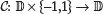by

$$C(d,j)=jd+\frac{5}{2}(1-j),$$

which is the identity on d when and which complements d when j = 1. Similarly, any configuration β and any position l within a binding site will correspond to a specific row of the PFM for the TF, depending on the orientation of the binding site; I denote this correspondence by a mapping ,

$$\begin{array}{c}(l,\beta )\underset{G}{\mapsto }\hspace{0.17em}\text{the index of the row of }c\hspace{0.17em}\text{corresponding}\\ \text{to position}\hspace{0.17em}l\in u(\beta ).\end{array}$$

Finally, in order to be able to model the joint probability of r and s, it will be necessary to count nucleotides of each type (ie, A, C, G, and T) outside of TFBS as well as at different positions within the binding sites of TFX. Outside of TFBS, I represent the nucleotide counts by the 4-vector f whose elements are defined by for all d ∈ . I represent the position-nucleotide counts for the sequence within all TFBS by a ω × 4 matrix σ whose elements are

$${\sigma }_{gd}=\left|\left\{l\in u(\beta )|G(l,\beta )=g\wedge c(r_l,J(l,\beta ))=d\right\}\right|$$

for all g ∈ and d ∈ . Because of the physical constraint that binding sites for TFX cannot overlap, it follows that for all g ∈ . In the next section, I introduce the statistical approach by defining a joint probability model.

Bayesian Approach to TFBS Enrichment Analysis

Having defined random variables to represent all of the observed information (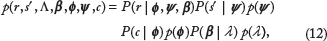R, C, S’) and the latent variables (Φ, Ψ, Λ), and the model parameter B, the first step in a Bayesian approach ⁴⁴ is to define a simplified model for the joint probability distribution. I choose the model

$$p(r,s^{\prime },\Delta ,\beta ,\varphi ,\Psi ,c)=P(r|\varphi ,\Psi ,\beta )P(s^{\prime }|\Psi )p(\Psi )P(c|\varphi )p(\varphi )P(\beta |\lambda )p(|\lambda ),$$

where the condensed notation P(λ) means P(Λ = λ) and so forth for the other random variables, P denotes a probability distribution, and denotes a probability density. Eq. 12 can be derived from first principles based on the following independence assumptions:

$$R\perp s^{\prime },C,\Delta |\varphi ,\Psi ,\beta$$

$$s^{\prime }\perp \Phi ,B,C,\Delta |\Psi$$

$$C\perp \Delta ,B,\Psi |\lambda$$

$$B\perp \Phi ,\Psi |\lambda$$

$$\Phi \perp \Psi ,\Delta$$

$$\Psi \perp \Delta$$

The independence structure of Eq. 12 can be summarized in graphical model notation, ⁴⁵ as shown in Figure 2. To make the joint probability model explicit, each of the conditional probabilities in Eq. 12 will be specified below.

Figure 2.

Graphical model diagram of the independence assumptions shown in Eqs. 13–18. Each arrow denotes a relationship between a parent variable and a child variable. Collectively, the variables and arrows indicate conditional independence as follows: each variable × is independent of other variables, jointly conditioned on all parents of X.

Modeling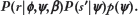

For PFM-guided computational recognition of TFBS, a fundamental assumption is that the probability model for the counts of nucleotides outside of TFBS is independent of the probability model for the counts of nucleotides within TFBS.^32,46 This means that the conditional probability of r can be expressed as the product of conditional probabilities for the subsequences of r corresponding to (the TFBS) and corresponding to (outside the TFBS). Conditioned on Ψ, the nucleotide probabilities at positions outside of TFBS, which are denoted by the random variables {R_l}_l∈Lr\u(β) and the random variables {S_l}_l∈L’, are assumed to satisfy for any l∈_r\U(β), and for any l ∈ ’ (where iid denotes independent and identically distributed). Conditioned on ϕ and β, the nucleotide sequence probabilities at locations within the footprint Û(β) of the binding sites specified by β, the nucleotide probabilities are denoted by random variables that are independent and distributed as follows: for any l∈_r\Û(β). Because the length of s’ is assumed to be quite substantial, the distribution of Ψ|s’ will be quite sharply peaked, and thus, any weak prior on Ψ will have little effect. Thus, it is reasonable to assume a uniform prior . Given the uniform prior assumption for Ψ and the definition in Eqs. 9 and 10 and the assumptions in Eqs. 19–22, the conditional probability of R, S’ has a compact form, that will be compatible with collapsing of ϕ and Ψ (as shown in the “Obtaining the distribution of ” section).

Modeling

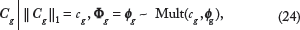
To account for uncertainty in the PFM due to sampling from a finite (and in many cases, very limited) number of representative binding site sequences, the PFM is represented by a random variable C. A core assumption in the field of PFM-guided TFBS recognition is that rows of C, denoted by C_g (where g ∈ ), are independent and multinomial distributed with a fixed number of trials.^47,48 Because in some cases, some representative binding site sequences will be outside the core portion of the multiple alignment from which the PFM is tabulated, the row sums of may in some cases be less than the count of representative binding site sequences. Thus, to accommodate such cases, I denote by the sum of the elements of row g of . In terms of the row-specific counts (for g ∈ ), the conditional distribution of C_g can be expressed as

$$C_g|{\Vert C_g\Vert }_1=c_g,{\Phi }_g={\varphi }_g\sim \text{Mult(}{c}_g\text{,}{\varphi }_{\mathrm{g}}\text{),}$$

for which the formula for immediately follows

The most common approach for selecting the prior probability for the PPM is to choose a uniform prior, in which case is just the constant (3!)^ω. Although other authors have pointed out the possibility of using an empirical prior on ϕ, ³⁰ it is nontrivial to collapse Φ by analytic integration over all ϕ, in the case of a nonuniform , so here I assume a uniform .

Modeling

At a given base pair location with no binding sites nearby (and with no sequence information), I model the probability that there is a binding site - in a specific orientation - as λ/2. In the absence of sequence information, intuition would suggest treating the occurrence or absence of a binding site for TFX at each position in DNA as independent and identically distributed Bernoulli trials. However, because of the physical constraint that two binding sites are not allowed to overlap, each binding site (ie, each nonzero entry of β) affects the probability of a binding site at nearby positions. Specifically, each binding site prevents the possibility of an overlapping binding site (in either orientation) at w - 1 bp positions, and for an additional 2(ω - 1) flanking positions, a binding site is only possible in one orientation. Thus, the probability model consistent with the physical constraints would be

$$\begin{array}{c}P(\beta |\lambda )=N_1(L_r,w,\lambda ){(\lambda /2)}^{\beta }{(1-\lambda )}^{L_r-w\beta -2(w-1)\beta }\\ \times {(1-\frac{\lambda }{2})}^{2(w-1)\beta },\end{array}$$

where is function that is implicitly defined by the law of total probability for P(β|λ). In the limit where L_r ≫ ω, and solving for N₁ using the law of total probability, we have the approximate result,

$$\begin{array}{c}P(\beta |\lambda )\simeq {\left(1+\frac{\lambda w{\left(1-\frac{\lambda }{2}\right)}^{2(w-1)}}{{(1-\lambda )}^{3w-2}}\right)}^{-\frac{L_r}{w}}\\ .{\left(\frac{\lambda {\left(1-\frac{\lambda }{2}\right)}^{2(w-1)}}{2{(1-\lambda )}^{3w-2}}\right)}^{\beta }+O(w/L_r).\end{array}$$

In the case ω = 1, the above can be seen to reduce to ${\lambda }^{\beta }{\left(1-\lambda \right)}^{L,-\beta }/2^{\beta },$ which is the expected joint probability of outcome sequence β for L_r independent trials of the categorical distribution with outcomes (-1,0,1) with probabilities (λ/2,1-λ,λ/2), in which β trials have a nonzero outcome.

The prior distribution reflects the range and relative probability of different Λ values for TFX, before the sequence r has been taken into account. The prior is important because for real-world applications, it can exert a significant effect on the distribution of Λ|r, c. For mammals, the prior can be formulated empirically using binding site frequencies (per base pair of noncoding, gene-vicinal DNA sequence) for 620 human TF ChIP-seq experiments (comprising 119 distinct TFs) obtained from the ENCODE project. ⁴³ For each ChIP-seq experiment, binding sites within regions of noncoding DNA within -1500 to +500 bp transcription start sites of VEGA transcripts (from Ensembl Release 75, GRCh37 assembly coordinates) were mapped, using ChIP-seq peak data that were peak-called using the SPP program ⁴⁹ and for which the data files were downloaded from the ENCODE data access page at the European Bioinformatics Institute from the June 2012 release (http://ftp.ebi.ac.uk/pub/databases/ensembl/encode/integration_datajan2011/byDataType/peaks/june2012/spp/optimal/) in narrowPeak format. The counts of binding sites within these noncoding regions were fit to a Poisson model parameterized by a binding site frequency λ per base pair of DNA; for each ChIP-seq experiment, a λ estimate was obtained using maximum likelihood. The resulting histogram of λ estimates is well-described by a beta distribution, as shown in Figure 3, with parameters as given in Table 2. Thus, it is convenient to adopt a prior density.

$$p(\lambda )=\frac{1}{B({\lambda }_{max};\alpha ,v)}{\lambda }^{\alpha -1}{(1-\lambda )}^{v-1},$$

where B is the incomplete beta function, and the shape hyperparameters are as given in Table 2 (recall that the range of Λ is (0,λ_max]). Combining Eqs. 27 and 28, and in the limit where $\lambda <\sqrt{L_r/w,}$ the product can be approximated

$$\begin{array}{c}P(\beta |\lambda )p=\frac{1}{2^{\beta }({\lambda }_{max};\alpha ,v)}{\lambda }^{\beta +\alpha -1(2w-1)\beta -1}\\ \times (1-O({\lambda }^2)),\end{array}$$

where with our choice of λ_max’ the second-order term can be neglected, resulting in a beta distribution-like dependence on λ,

$$\begin{array}{c}P(\beta |\lambda )p(\lambda )=p(\beta ,\lambda )=\frac{1}{2^{\beta }({\lambda }_{\max };\alpha ,v)}{\lambda }^{\beta +\alpha -1}\\ \times {(1-\lambda )}^{v+L_r-(2w-1)\beta -1},\end{array}$$

for λ∈(0,λ_max] From this equation, and integrating λ over the range from [0,λ_max], we see that the probability model Eq. 26 corresponds to a prior

$$P(\beta )=\frac{B({\lambda }_{max};\beta +\alpha ,v+L_r-(2w-1)\beta )}{2^{\beta }B({\lambda }_{max};\alpha ,v)}.$$

Figure 3.

Distribution of frequencies of TFBS (per base pair of noncoding, gene-vicinal DNA sequence) for human transcription factors, based on the analysis of 620 ChIP-seq datasets from the ENCODE project. ⁴³

Table 2

Parameter estimate for the beta distribution model for the prior p(λ) on the binding site frequency per base pair, for human transcription factors.

	a	V (X104)
Least-squares estimate	1.37	3.62
95% confidence interval	∓0.15	∓0.53

In contrast to Eq. 31, Lähdesmäki and Shmulevich ⁵⁰ used a geometric prior on, βp(β) = 1/2^β+1, implying

$$P(\beta )=q\frac{B!(L_r-\beta )!}{L_r!}\frac{1}{2^{\beta +1}},$$

up to a normalization constant q. A comparison of the two priors (Fig. 4) suggests that the incomplete beta function prior (Eq. 31) may be more conservative than the geometric prior - a hypothesis that I investigate by analyzing simulated promoter sequence data in the next section.

Figure 4.

Plot of the change in log P(β) with the addition of a single binding site, as a function of β, for the incomplete beta function-based prior (Eq. 31) and the previously proposed geometric prior (Eq. 32). The △logp values between the two priors are closer for β = 0 but become greater with increasing β, indicating that the empirical prior in Eq. 31 is not simply equivalent to a rescaling of the geometric prior.

Obtaining the Distribution of B|r, s’,c

The second step in a Bayesian approach ⁴⁴ is to condition on the observed data - in this case, r, s’, and - and then obtain the conditional distribution of the parameter(s) of interest, in this case B. In order to be able to do so, starting from the joint probability model (Eq. 12), the nuisance parameters ϕ and λ must be either estimated or marginalized. A key advantage of the Bayesian approach is that we can take into account the probability distribution of , in the process of eliminating Φ by marginalization. The parameter Ψ can be similarly marginalized, although the uncertainty in the background nucleotide frequency is generally very small for real-world applications in which L’ is large. We marginalize ϕ and Ψ by integration,

$$p(r,s^{\prime },\lambda ,\beta ,c)=\int d^{3w}\varphi \int d^3\Psi \hspace{0.17em}p(r,s^{\prime },\lambda ,\beta ,\varphi ,\Psi ,c).$$

Given Eqs. 12, 23, and 25, the dependence of the integrand in Eq. 33 on ϕ and Ψ has the same algebraic form as the probability density function for independent Dirichlet random variables {Ψ,Φ₁,…,Φ_ω} as a consequence of the fact that the Dirichlet distribution is the conjugate prior for the multinomial distribution. ⁴⁴ Thus, the two integrals in Eq. 33 can be evaluated analytically. ³⁰ The desired joint conditional probability of Λ, B follows by the definition of conditional probability,

$$p(\lambda ,\beta |r,s^{\prime },c)=\frac{p(r,s^{\prime },\lambda ,\beta ,c)}{P(r,s^{\prime },c)}.$$

After performing the integrals in Eq. 33, using Eqs. 30 and 34, and then log-transforming, we have where is function that will not need to be evaluated. The parameter λ can then be marginalized by integration, yielding where B is the incomplete beta function. As we will see below, in order to obtain samples of , it will not be necessary to explicitly evaluate . Now that we have an explicit formula for up to additive terms that do not depend on β, it is possible to generate β samples from this distribution using Markov Chain Monte Carlo (MCMC) sampling.

MCMC approach

For sampling from , the Metropolis-Hastings algorithm, ⁵¹ in which a probabilistic proposal generator g(β,β’) for a transition from β→β’ can be defined so as to optimize the acceptance rate for moves, is convenient. For the problem of TFBS enrichment detection, following the general approach used by Lahdesmaki et al for TFBS recognition, I use a two-stage proposal generator in which a base pair position l ∈ _r is selected at random, and then, depending on the current state of β, binding site removal or addition (in the latter case, with a randomly selected value j ∈ {-1,1}) is proposed (in the case of binding site addition, j = -1 or j = 1 is chosen with equal probability). For this approach, it will be useful to have a simplified expression for the log probability ratio for B_l = j versus B_l = 0, conditioned on r, s’, β_r\[l] it is convenient to define some additional notation in order to make this conditional probability ratio explicit. Without loss of generality, let us assume that the current state for the hypothetical binding site configuration β ∈ , a location l ∈ _r such that β_l = 0, and an orientation j ∈ {-1,1} such that the configuration β with β_l = j would not violate the TFBS physical constraints. In order to simplify notation, I define a function H:^L_r × × {-1,1} × → by

$$H(r,l,j,g)=C(r_{l+j(g-1)},j),$$

whose value represents the nucleotide at position g within the binding site for TFX that has orientation j and whose 5’ most nucleotide is at location l ∈ _r I also define a function by whose value is the count of nucleotides of base d within a binding site for TFX in orientation j whose 5’ most nucleotide is at location l.

Applying Eq. 35 to two different binding site configurations that differ by one binding site being present/absent at a specific location l ∈ _r, and using the definitions of and , we obtain a closed-form expression for the log ratio of the conditional probability of there being a binding site at location l (in orientation j), to the conditional probability that there is not a binding site at l where the notation (x)_[n] denotes the falling factorial and σ is computed for β. Given Eq. 39, sampling from the distribution of can be accomplished using the Metropolis-Hastings algorithm with the following proposal distribution: where S_l is the Shannon entropy of the probabilities , and where the weight exponent q is tuned to achieve the desired average acceptance rate. ⁵² The reason for using a proposal distribution that weights each position by the Shannon entropy is that at most positions , the entropy of the three conditional probabilities and fixed l) is very small, and thus, from the standpoint of optimizing the acceptance rate, it is convenient to weight the generation of proposed moves toward moves with more even odds of move acceptance. Results from empirical testing with sequence lengths L_r = 2 × 10⁴ suggest that a value q = 0.85 gives an acceptance rate of about 0.12, with increasing values of q increasing the acceptance rate. In this study, the Markov chain is initialized by iterating over l = 0 to l = L_r, for each l, setting β_l to be the most probable configuration given Eq. 39, conditioned on β_r\{l} 0. Once the Markov chain has converged, at most positions l ∈ _r, the entropy of the three conditional probabilities and fixed l) is very small, and thus, from the standpoint of optimizing the acceptance rate, it is convenient to weight the generation of proposed moves toward moves with more even odds of move acceptance.

Empirical Results

Based on a direct comparison (Fig. 4) of the incomplete beta function prior (Eq. 31) and the previously proposed geometric prior (Eq. 32), it seems reasonable to suppose that, within the context of a Bayesian approach for PFM-based TFBS frequency estimation (as described in the “Obtaining the distribution of ” section) the incomplete beta function prior and the geometric prior might have different effects on the conditional distribution of the number of TFBS, ie, the samples of B|c, r, s’. To test this hypothesis, I generated a synthetic dataset based on a simulated background sequence s’ (with L’ = 100,000) and 120 gene promoter sequences (each with L_r = 20,000), with uniform probabilities for each nucleotide. Into each simulated base sequence r, and for each of a fixed set of 100 TF PFMs selected at random from TRANSFAC Professional 2015, t ∈ {1, …, 10} TFBS were inserted into the r sequence (using representative binding site sequences from which the PFMs were computed, resulting in a modified sequence rt). Ten samples from the stationary distribution of B (the number of TFBS) were then generated using the MCMC approach described in the “MCMC approach” section (with 5000 burn-in steps, 100 steps per sample, and q = 0.85), for both the geometric prior and the incomplete beta function-based prior (with v = 10,000 and α = 1.0). For each of the two priors and for each combination of sequence r, PFM c, and number of ground-truth binding sites t, the 10 B|c, r_e, s’ samples were averaged, producing one geometric prior sample and one incomplete beta function prior sample for each of the 120,000 combinations of c, r, and t. The distributions of B|c, r_t, s’, organized by t and by prior, as shown in Figure 5, reveal several interesting patterns. First, across the fixed set of 100 randomly selected TFs, the MCMC method incorporating the incomplete beta function prior appears to yield samples that are more accurate than the MCMC method incorporating the geometric prior. In terms of mean-squared error, the MCMC method with the incomplete beta function-based prior is 19.6, whereas the mean-squared error with the geometric prior is 107.7. Second, the samples generated using the MCMC method with the geometric prior appear to be substantially higher-variance than the samples generated using the MCMC method with the incomplete beta function-based prior (quantitatively, the t-averaged standard deviation of the TFBS count samples obtained using the incomplete beta function prior was 4.05 versus 8.75 for the geometric prior.

Figure 5.

Comparing the accuracies of two MCMC implementations of the Bayesian method for estimating the number of binding sites of a TF, based on the geometric prior (Eq. 32) and the incomplete beta functionbased prior (Eq. 31). For each combination of t (number of ground-truth sites) and type of prior, the bar denotes the median, the box denotes the interquartile range, and the whiskers are offset 1.5 interquartile range above or below the 75th and 25th percentiles.

Discussion

This study demonstrates the utility of incorporating an empirical prior on the TFBS frequency per base pair within the context of a Bayesian method for PFM-based TFBS enrichment analysis, but there are several aspects in which the work raises interesting questions that could be explored in future studies. First, in this work, a two-parameter parametric function has been fit to empirical data on the density distribution of frequencies of human TFBS per base pair of noncoding, gene-vicinal sequence. Thus, the results shown here do not reveal to what extent the estimated parameters for the distribution would generalize to TFBS frequencies in other species. At least for the mouse genome, available evidence from the modENCODE project suggests that overall, TF binding within promoter regions is highly conserved between human and mouse. ⁵³ Moreover, for two TFs whose TFBS were assayed in five mammalian species by ChIP-seq, the numbers of genome-wide binding sites did not vary more than 2x between species. ²² Thus, it seems reasonable to expect that the A prior distribution (across TFs) would be similar, for gene-vicinal non-coding sequence. Nevertheless, in future work, it would be informative to estimate the hyperpriors a and V for human, mouse, fruit fly, and worm to enable a cross-species comparison. Second, it would be useful to characterize how the choice of q parameter affects the empirical performance of the MCMC approach used here, ie, the acceptance ratio, the number of steps required for burn-in, and the number of steps required between samples; it may be possible to significantly improve the speed of the proposed MCMC method through tuning q and the sampling parameters. Third, a key aspect to be explored is the extent to which the accuracy improvement with the incomplete beta function-dependent prior is associated with high-count versus low-count PFMs. Intuitively, it seems reasonable to suppose that for most TFs, an increase in the accuracy of the prior would be expected to have more of an effect on the posterior distribution of β when the PFM count is low, since a higher count PFM would be expected to have a much bigger likelihood ratio that would, in turn, be more likely to dominate over the prior on the number of TFBS.

Conclusions

This study presents a Bayesian approach to the bioinformatics problem of PFM-guided TFBS enrichment analysis. The method incorporates an empirical prior on the frequency distribution λ of binding sites for TFs that is based on genome location data from the ENCODE project. In addition, the method incorporates a probabilistic model for TFBS occurrence conditioned on the parameter λ that takes into account the finite width of the TFBS, in contrast to a previous approach in which the TFBS probability was assumed to have a geometric dependence with a fixed factor of 1/2. ³⁰ The sampling equation for adding/removing a binding site (Eq. 39) could be easily extended to include other sources of information, such as a regulatory potential score derived from phylogenetic sequence conservation or from epigenetic measurements. The R software code implementing the MCMC method described in the “MCMC approach” section and the promoter analyses shown in Figure 5 is available at http://github.com/ramseylab/tfbsincbeta.

Author Contributions

Conceived and designed the experiments: SAR. Analyzed the data: SAR. Wrote the first draft of the manuscript: SAR. Contributed to the writing of the manuscript: SAR. Agree with manuscript results and conclusions: SAR. Jointly developed the structure and arguments for the paper: SAR. Made critical revisions and approved final version: SAR. The author reviewed and approved of the final manuscript.