
Abstract
In this study, we introduce an artificial intelligent method for addressing the batch effect of a transcriptome data. The method has several clear advantages in comparison with the alternative methods presently in use. Batch effect refers to the discrepancy in gene expression data series, measured under different conditions. While the data from the same batch (measurements performed under the same conditions) are compatible, combining various batches into 1 data set is problematic because of incompatible measurements. Therefore, it is necessary to perform correction of the combined data (normalization), before performing biological analysis. There are numerous methods attempting to correct data set for batch effect. These methods rely on various assumptions regarding the distribution of the measurements. Forcing the data elements into pre-supposed distribution can severely distort biological signals, thus leading to incorrect results and conclusions. As the discrepancy between the assumptions regarding the data distribution and the actual distribution is wider, the biases introduced by such “correction methods” are greater. We introduce a heuristic method to reduce batch effect. The method does not rely on any assumptions regarding the distribution and the behavior of data elements. Hence, it does not introduce any new biases in the process of correcting the batch effect. It strictly maintains the integrity of measurements within the original batches.
Introduction
Opening remarks
The large-scale transcriptome data obtained from microarray or RNA-Seq experiments usually consist of biological signals of interest, conditional covariance and biases associated with batch effect, originating from different technical conditions. Batch effect can be referred to the transcriptional differences due to nonbiological issues such as: different laboratory operating procedures, differences in RNA isolation, amplification and hybridization, differences in scanner type, settings, calibration drift, etc. These batch-associated background differentials lead to systematic and nonystematic, nonbiological differences in gene expressions and thus creating the need for a preprocessing data preparation stage aimed to reduce batch effect as much as possible, while avoiding the introduction of new biases in the process.
Our study is addressing the process of data correction to reduce batch effect. There are numerous methods to normalize high throughput expression data, but all these methods rely on assumptions regarding the data distribution and behavior. These assumptions are usually tailored toward the requirements of the methods applied in the preprocessing and later analysis. In the literature survey covered in our study, we found no extensive elaboration and discussion regarding the consequences of the original data being substantially different vs the assumptions made. Moreover, to accommodate the preassumed conditions, some of the methods generate normalized data that substantially deviate from the characteristics of the real data. We must keep in mind that batch-effect removal is only a preparation stage for the actual medical or biological research, which will follow. Hence, the normalization process must be conducted as carefully as possible, while minimizing the danger of causing data distortions. It is preferable to leave some minor batch effect uncorrected rather than fundamentally distorting the distribution of the data to fit it into required framework of various data processing methods.
Overview of our approach
To address the issue raised above, we introduce an entirely different concept of normalization to handle the batch effect. The main issues introduced in our study are as follows:
There are no theoretical proofs indicating that the expressions of each gene across the multiple samples must be distributed according to 1 type of distribution or another. Therefore, no assumptions regarding possible distribution of transcriptional measurements within each gene are made.
There are no theoretical proofs indicating that gene expressions of each gene across samples must be distributed in a similar way across the various genes. Thus, our method attempts to correct the batch effect for each gene independently and unrelated to other genes.
The method introduced here is intuitively simple enough, so that medical-biological professionals will be aware of what is done and what is the meaning of the resulting normalized data.
The way the “Batch Effect” is defined, there are no scientifically proven tools to measure it. There are also no scientifically proven and accurate enough methods to measure a degree to which the batch effect is eliminated. Even if there are studies that are claiming that their methods are capable of eliminating the batch effect entirely, it can be claimed only based on their own assumptions. We are not claiming that the introduced method completely eliminates the batch effect. The method will reduce batch effect to the greatest degree possible, while causing minimal data distortions. It is preferable to have some remains of the batch effect, while maintaining the integrity of the original data.
In numerous studies presented in the literature (see “Related Work”), the data go through several transformations until becoming ready for the main purpose: medical or biological research. For example, SCAN transformation aimed to increase signal-to-noise ratio within individual sample performed, following the gene expression measurements. Some methods use logs transformation of raw data. Furthermore, in addition to the “Batch” normalization process, some studies conduct additional data adjustments to prepare the data for the requirements of the methods used for further research. Each such step involves potential distortion to some degree and the cumulative effect of all of them is very difficult to assess. Due to these reasons, our method conducts batch normalization directly on the original raw data, and the resulting data are ready for medical/biological modeling.
Main principles and components of the system
The major components and the procedures of our system are as follows:
Data. We use raw data without any preprocessing modifications. We use well known data mining algorithm (the dynamic k-mean algorithm) to divide the data of each gene into clusters. It is easy to observe by comparing clusters of various genes that the distribution of data is definitely not uniform, and the assumption of uniform data distribution across genes is artificial and incorrect.
Reference point. Every normalization method requires selection of a reference point, based on which the data are adjusted. Any point can be selected as a reference point, and the normalizing process is considered legitimate as long as it is consistent, logical and preserves data integrity (does not introduce biases in the process). The method presented here selects the reference point based on the center of gravity of the main concentrations of data elements (of a specific gene). The main idea is to select the reference point in the area where most of the data elements are located, and then during the normalization process, most (more than 50%) of the data elements will not be changed substantially, especially if the whole batch is located in that region. Only batches that are located further from such selected point will require more drastic adjustment.
Selection of the reference point. The process of selecting the reference point for each gene is as follows:
3.1. First, we find the cluster that contains the most data elements in comparison with other clusters.
3.2. Then, the algorithm selects a contiguous group of clusters (which includes the cluster having largest amount of elements), such that the amount of all the data elements for the whole group exceeds 50% of the total amount of data elements. We name such concentration of data CGCG (Central Gravity of a Cluster Group). The central tendency (or center of gravity) of CGCG will represent the point of reference for the batch normalization process. The idea is that when trying to identify the point of reference for the normalizing process, we are addressing the center of gravity of the main concentration of the data elements, and not the center of the whole data, which could be substantially affected by the batch effect. We find the center of gravity (median) of the CGCG, which becomes a point of reference for the normalization.
Center of gravity for each batch. We must keep in mind that some batches are very small (consist of only few data elements—some have only 2 elements). Obviously, finding center of gravity for such small batches by selecting their median will be highly unreliable. Hence, we use the set of clusters containing that batch. If all the samples of a given batch are located in 1 cluster, then we select cluster’s median as the center of gravity for the batch. If a batch is spread over several clusters, we find the cluster containing the smallest numerical value (of gene expression) of the batch, and the cluster containing the largest numerical value of the batch. Those 2 clusters and all the clusters between them will constitute the relevant data group for the batch. We name the group “Batch Cluster Group” (BCG), and the median of the whole group will represent the center of gravity of the batch.
Recalculation the values. Once we have the center of gravity of the main concentration of the gene data, and the center of gravity of the batch, we can find a ratio between those values and use it to recalculate the values of the data points for that batch.
Related Work
There is a vast literature addressing the batch normalization options. The following is a brief survey of literature relevant to our method.
Liu et al 1 presented a fairly extensive survey of the better-known methods for data preprocessing (normalization methods) for unbalanced transcriptome data. The authors briefly presented 23 methods and they stated, that among the methods surveyed, no method is without some assumptions. Each of the methods surveyed is based on its own assumptions, implying corresponding problems. Another important point that must be kept in mind—the methods surveyed in the article do not necessarily deal specifically with the batch effect. They involve various data preprocessing methods designed to prepare the data for further biological analysis, which is the final and the most important objective. For example, the authors mention the CrossNorm method, as one of the most effective data normalization methods. However, Cheng et al, 2 who introduced the method, clearly stated that all the samples are required to be from the same batch.
In our study, we limit the scope of data normalization to batch effect only. In our judgment, it is preferable to address each type of bias correction separately, and attempt to correct several types of biases in combination only if intuitively, the same type of correction process is applicable to all of them. Otherwise, it is preferable to separate the data preparation procedures into separate processes, each as simple as possible, and as intuitive as possible.
One of the most effective and widespread methods to address the batch effect was introduced by Johnson et al.
3
The method eventually became known as ComBat. The method is based on the Empirical Bayes and involves some assumptions regarding the data. The error terms are assumed to follow a normal distribution with expected value of zero and variance
In ComBat method, the first step is to standardize the data, so that genes have similar overall mean and variance. The method assumes that batch effect usually affects many genes in similar ways (ie, increased expression). The parameters that represent batch effect are estimated by pooling information across genes for each batch. These Empirical Bayes estimates are then used to adjust the data elements for the batch effect. Johnson et al. 3 did not evaluate the consequences of using their method in those cases where the data do not correspond to the various assumptions they made.
Chen et al 8 compared and evaluated several different methods to adjust the data for the batch effect. The testing was made based on measures of precision, accuracy, and overall performance, as defined by the authors. ComBat, an Empirical Bayes method, outperformed the other methods by most metrics. The methods compared were as follows:
DWD (distance-weighted discrimination), 6 based on the support vector machines (SVM) algorithm. DWD did not perform well when batch sizes were small. In addition, it can only analyze 2 batches at a time. Three or more batches may still be adjusted with DWD, using a stepwise approach 6 (very inconvenient in large data sets).
PARM (mean-centering) 9 which is based on gene-wise 1-way analysis of variance (ANOVA). The method sets the mean of any given batch to zero. It performed very well in terms of accuracy. PARM does treat all samples equally, so it can over-correct or under-correct specific samples and it came second after ComBat, based on criteria as defined in the study.
SVA (surrogate variable analysis), 10 combines singular value decomposition (SVD) and a linear model analysis to estimate the eigenvalues. Its limitations: it is not easy to identify the batch effect eigenvector. Thus, SVD may not identify and remove all the batch effects, and may remove other effects not related to batch. In addition, the basic assumption of SVD is that the eigenvectors have Gaussian distributions—this assumption does not always correspond to the actual data. Also, SVD is not robust to outliers when compared with an Empirical Bayes method.
Geometric ratio-based method (Ratio G) scales sample measurements by the geometric mean of a group of reference measurements. 11 Luo et al 11 demonstrated that Ratio G outperformed other methods in adjusting data for use in a predictive model, however, by accuracy Ratio_G performed worse than ComBat.
An Empirical Bayes method, (ComBat), 3 estimates parameters for location and scale adjustment of each batch for each gene separately. This methodological approach reduces batch effects and raises precision and accuracy. The ComBat method outperformed the second-best method by a substantial margin. Unlike the other methods, each of which had at least one major drawback, ComBat performed satisfactorily on all measures. The contrast in performance between ComBat and the other methods increased with decreasing of batch size, suggesting that this Empirical Bayes approach is particularly appropriate for studies with fewer samples per batch. PAMR was a close second, but its performance was impaired with small batch size; only ComBat performed robustly when adjusting small batches, (hence motivating us to compare our algorithm with ComBat).
Stein et al 12 introduced modified ComBat (M-ComBat) that shifts samples to the mean and variance of the “gold-standard,” which is a reference batch, instead of the grand mean and pooled variance.
Therefore, the authors postulate that the Modified ComBat eliminates batch effect related differences while adjusting all samples to a predefined standard. The standardized data are assumed to be normally distributed, and the ordinary least-squares are used to calculate gene-wise mean and standard deviation estimates.
Müller et al 13 presented another comparison of various methods for batch effect correction. They compared 7 methods: (1) Deming regression, 14 which allows to model normally distributed errors; (2) Passing-Bablok regression, 15 that does not introduce assumptions regarding the underlying error distributions; (3) Linear mixed models; (4) Third-order polynomial regression; (5) Nonlinear method qspline, 16 that integrates quantile information of gene expression distributions and uses a cubic spline to fit all values dependent on signal intensities; (6) ComBat (based on empirical Bayes); 3 (7) Matrix factorization-based method for the cases where unwanted factors of variation are unknown, the background noise is modeled by negative control genes. Removal of unwanted variation (RUV) uses negative controls combined with technical replicates when estimating and correcting for batch effects (ReplicateRUV). 17
Each method was first tested on raw log2-transformed data and, in a second step, the tests were repeated following the quantile normalization of the batches. Deming regression, Passing-Bablok regression, linear mixed models, and nonlinear approaches (third-order polynomial regression and the nonlinear method qspline) did not adequately reduce the batch effects. When focusing on the data set of sample replicates, ReplicateRUV outperformed ComBat in terms of batch effect removal and retention of biological variation.
However, when batch effect removal was applied on the entire data, quantile normalization followed by ComBat performed better in comparison with quantile normalization followed by ReplicateRUV or ReplicateRUV without quantile normalization. Various values of ReplicateRUV parameter k (which represents an estimate of the amount of the unwanted factors) were tested. The results did not substantially improve batch effect removal. Therefore, quantile normalization followed by ComBat came out as the most successful approach among the methods tested.
Indeed, combination of Quantile normalization and ComBat is superior over ComBat alone, and Quantile normalization diminishes variances within each batch and supports ranking of genes.
Weishaupt et al 18 attempted correction of batch effects of cerebellar and medulloblastoma (MB) gene expression data sets, using the RUV algorithm. 19 The authors claimed that ComBat3 and SVA 20 use batches as covariates, might face problems in distinguishing between batch effects and biological differences, or might artificially increase differences between phenotypes.21,22 Weishaupt et al 18 claimed that in their study, such difficulties were expected to be relatively stringent, because tumor and normal samples are broadly separated into unique batches. Therefore, they decided to use the RUV method 19 that can correct for batch effects via negative control genes (NCGs). This method needed further knowledge about NCGs that are assumed to obtain almost constant expression between any of the experimental conditions. House-keeping genes were suggested as one potential source of internal controls. 19 However, given that such genes are typically presented with high expression across normal adult tissues, 11 they are not generically applicable to MB. Therefore, batch correction was performed via the naïve RandRUV method. 17 A visual analysis of the relevant dataset demonstrated reducing of batch effect observed in the raw data. A problem with this technique is the lack of golden standard NCGs. The authors overcome this problem by implementing empirical estimation of NCGs. They concluded that the choice of NCGs has a definite effect on the whole process.
Weishaupt et al 18 also addressed the question of how to estimate the existence of batch-effects and measure the data normalization performance. They concluded that the choice of evaluation metrics is perhaps just as crucial as the choice of NCGs, and that variable methods need to be combined to address different aspects of data quality affected by batch effects.
Zhang et al 23 suggested various enhancements to the ComBat method. Similarly, Stein et al 12 (who advocated applying the “Gold Standard” batches in the process of normalization) suggested selecting a batch of superior quality as a natural “reference.”
They argued that the standard ComBat suffers from the problem of “set bias,” 24 meaning that when batches are added to or removed from the data, the normalization procedure must be reapplied, and the resulting values are expected to be different—even for the batches that remained in the data set in various scenarios. Once the test sets are available and combined with the training data, then following the application of ComBat, the training data may change, which makes it necessary to regenerate biomarkers. As ComBat modifies the variance for each gene, it is expected to generate different test statistics, which in turn is expected to result in increased or reduced P value. All this tends to cause some genes to be included or excluded from the biomarker list, thus leading to a different biomarker. If ComBat is applied to several training/test data combinations separately, then the resulting biomarker is expected to be different among these data sets. Hence, the authors emphasize the importance of establishing the training set as a “reference data set,” to which all future batches will be standardized. This allows the training data and biomarker to be fixed in advance while making it possible to apply the biomarker to any amount of additional sets. This idea is especially effective in situations where one batch or data set is/are of more reliable and stable in comparison with others.
Zhang et al 23 also offered improvements of ComBat method on the technical level. They commented that ComBat assumes error term having normal distribution with expected value of zero and variance σ2. The original ComBat method uses all samples to estimate the mean and the variance of batch effects, which leads to a correlation between the samples. Such correlations may cause problems, such as inflating type I error in differential expression detection, if not applied and interpreted properly. In addition, the authors observed evidence in all 4 data sets they tested that their ComBat based model did not completely remove all batch effects.
Therefore, the authors suggested a more complex testing, involving in addition to mean and variance, also skewness and kurtosis. The proposed improvement was based on assumptions of exchangeability across genes regarding the mean, variance, skewness, and kurtosis.
Zindler et al 25 discussed the problem of P value inflation with subsequent false positive results when applying the popular ComBat method. They claimed that utilizing ComBat to correct for batch effects produced substantial magnitude of false discovery rate (FDR). Batch effects tends to substantially reduce the accuracy of measurements, 26 and the use of ComBat to mitigate batch effect can lead to false-positive results, if the sample is not uniformly distributed.
This can lead to group differences caused by measurement errors being wrongly associated to the outcome of interest.27,28 Zindler et al, 25 by full-text search provided in Google Scholar since 2018, identify 54 studies which employed ComBat in their statistical analysis. Unfortunately, none of these studies provided necessary details regarding their batch factor structure, sample distribution, and other ComBat parameters to enable to recreate their analyses. 72.73% of authors merely report that ComBat was used, while the other studies stated the corrected factors, but missed other important information related to the exact number of factors or sample distribution.
Zindler et al 25 indicate that the use of ComBat for batch effect reduction can lead to any false significant results. Their results strongly support the important warnings made by other authors to double-check every step of the process using ComBat for batch effect correction especially on unbalanced samples.21,29,30,31
The Batch Effect Correction Heuristic Algorithm (BECHA)
Let
First, we sort the data (for each gene) in an increasing order. Then, we divide the data into clusters using a variation of the dynamic k-means clustering algorithm (see Algorithm 2 in Yosef et al,
32
in addition, interested reader can see the Algorithm in the appendix). The result of this process is the creation of r clusters:

Step 1—create clusters for each gene.
In our method, the reference point for normalization is defined as the central tendency (center of gravity) of the main concentration of data in each gene, and consists of contiguous group of clusters containing more than 50% of the data elements. The reference point is not based on the whole data to minimize influence of the batch effect on the selection.
To locate the concentration of clusters containing the majority of measurements per gene, the following steps are taken:
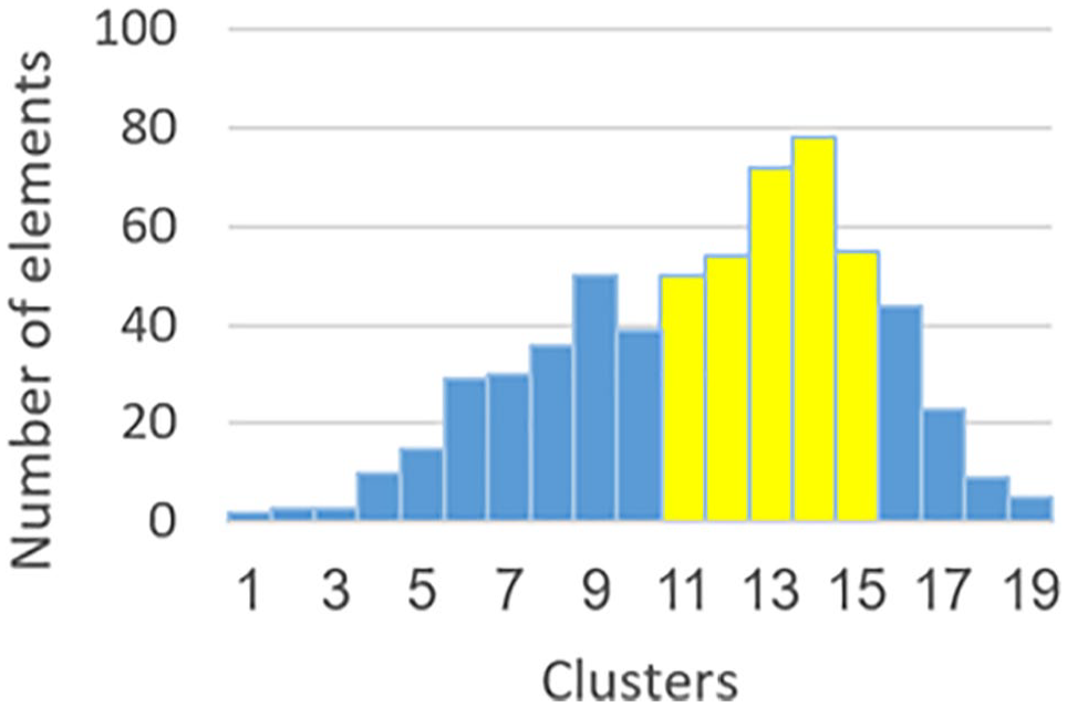
We locate a cluster containing the largest amount of data elements (cluster 14 in Figure 2). This cluster becomes first component of CGCG.
Enlarging CGCG until total amount of data elements in the group constitutes a majority of the gene’s data. We are comparing the cluster located to the left of CGCG and to the cluster located on the right side of CGCG (in Figure 2—cluster 13 is compared with the cluster 15). The larger cluster is merged into CGCG (in our example, it will be cluster 13). The process continues until CGCG contains more than 50% of gene’s data (in our example: clusters 11-15).
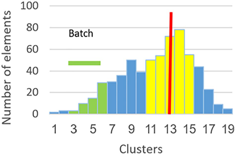
Step 3 consists of computing a central tendency point for CGCG. We use the median as the representative of central tendency, to avoid influence of outliers. In Figure 3, the red bar represents the median.
Step 4 involves finding the BCG, which is a group of clusters containing a given batch. Some batches are very small (having 2 data elements), and therefore, finding central tendency of small batches will be unreliable. Thus, to find central tendency of a given batch, we use contiguous data of all the clusters containing a given batch. In our example (Figure 4), the minimum gene expression of the batch is located in cluster 3. The maximum gene expression of the batch is located in cluster 6. In this case, BCG will consist of the clusters between 3 and 6, inclusive (colored in green).
Step 5: In the overwhelming majority of cases, the amount of data in BCG is large enough for reliable computation of the central tendency. We compute the median of BCG to avoid influence of outliers (see brown bar in Figure 5).
The final step (Figure 6) in the normalization process is to compute the new values for batch’s data elements. First, we compute the ratio between the centroid of the BCG and the centroid of the CGCG. This ratio is applied to every data element in the batch to move it toward the centroid of CGCG.
Step 2—find the Central Gravity Cluster Group.

Step 3—compute the centroid of the CGCG. CGCG indicates Central Gravity Cluster Group.
Step 4—find the Batch Cluster Group (BCG).

Step 5—compute the centroid of the BCG. BCG indicates Batch Cluster Group.

Stp 6—normalization process.
Notes
Important feature of the normalization process is the preservation of the integrity of the data, which means that the ratios among the values of data elements within a batch remain the same (unlike some other methods such as ComBat).
The method is heuristic and intuitively very simple.
No assumptions are made regarding the data distribution within a given gene, or across genes, within a given batch or across the batches.
Algorithm 1: the batch effect correction heuristic algorithm (BECHA)
Input:
Output: Normalized matrix of the genetic expression data.
For each gene
Sort genetic expressions of the gene
Create clusters for gene
Find the Central Gravity Cluster Group (denoted by
For each batch
a. Create batch cluster’s group (denoted by
For each data element
Algorithm 2: the Central Gravity Cluster Group of gene
Input: Set of clusters
Output: The
1. Find cluster
2.
3.
4. While
If
Else (ie,
5.
6. Compute the centroid of
Algorithm 3: the batch cluster’s group
Input: Batch
Output: The batch cluster’s group (
Find cluster containing
Find cluster containing
Compute the centroid of
Addressing various distributions of gene’s data elements
In the previous section, we described the heuristic normalization process. The first step of the process was to divide the data of a gene into clusters. When applying cluster construction procedure, we used parameters that allow the system to divide the data of each gene into no more than 20 clusters, for reasons explained above. When observing the general patterns of clusters’ histograms, we notice, that for a majority of genes, there is a largest cluster (containing the largest amount of data), and the neighboring clusters generally decline as we move away from the largest cluster. The decline is not monotonic, there are ups and downs, but the general trend is declining. When the largest cluster is on the edge of the histogram, then the decline is one-sided.
However, not all histograms behave as described above. There are cases where clusters decrease, reach some minimum, and then turn around and begin to rise again. The increase continues until some local maximum is reached, and then the downward trend begins again. In other words, there are 2 distinct groups of data elements (see Figures 7A and 7B).

(A) 2 distinct groups of data elements 1. (B) 2 distinct groups of data elements 2.
The separate groups of the data points, as described above, can be easily justified. It means that in some genes, genetic expression for one group of individuals significantly differs from another group. For example, group affected by a given illness vs healthy group, or group of ill patients who were treated with a given medicine vs a group that was not treated. However, genetic data could be split into groups by coincidence due to a batch effect—in particular when the additional group is (groups are) small.
The greatest challenge of data preparation is to remove the consequences of batch effect to the greatest degree possible, while maintaining distinction between groups where such a distinction is justifiable. Hence, it becomes necessary to design a normalizing process that will distinguish to the best degree possible between the separate groups (where such separate groups exist), and not treat them as if they are 1 group.
When a separate group is a result of batch effect, then it is necessary to address the whole data of both groups as 1 group, and to apply batch removal normalization for the entire data of these groups. However, when there are 2 (or more) justifiably distinct groups, then the process of normalization becomes more complicated. Because all the groups are still affected by batch effect, batch adjustment must be performed. Nevertheless, to maintain the distinctiveness of these groups, each group will have to be normalized separately (using the same algorithm as described in the previous section).
When normalizing a gene characterized by data divided into groups, the major challenge is to distinguish between a group coincidentally created by the batch effect from a group that truly and justifiably can be defined as separate. For that purpose, it is necessary to design heuristic rules that will allow us to distinguish between these 2 cases. In this study, we used 2 heuristic rules as follows:
Rule 1: If the distinct group is small enough, then it is most likely the result of a batch effect, and such a group should be treated as an integral component of the larger group. The measurement in this case is a percentage of data elements within the smaller group vs total population of the data elements (in a given gene).
Rule 2: The magnitude of the peak (the largest cluster of the additional group) vs clusters of the dominant group (where the global maximum cluster is located).
For rule 1, the question becomes, how to determine, when the group is small enough. To determine such benchmark, the same clustering algorithm was applied, using nonhuman genes/probes associated with Eukaryotic Poly-A RNA Controls supplied in the GeneChip 3 IVT Express Kit. The nonhuman genes cannot be considered (as compared with human genes) affected by some diseases associated with humans, or affected by some medical treatment, etc. Therefore, any distinct group of data elements is considered as being a result of a batch effect. We observed the largest magnitude of such group (as a percentage of total data points [per gene]) and found that for nonhuman genes, the separate, supposedly batch-caused groups do not exceed 10% of the total elements of the gene. Hence, we used 10% as a benchmark in the first heuristic rule. In other words, if there is a separate group of data points, and they are 10% or less vs the total amount of data for that gene, then we consider the smaller group as being a result of batch effect. Figure 8 illustrates rule 1: the group of data elements consisting of clusters 14 through 19 is less than 10% of the total amount of data elements in clusters 1 through 19.
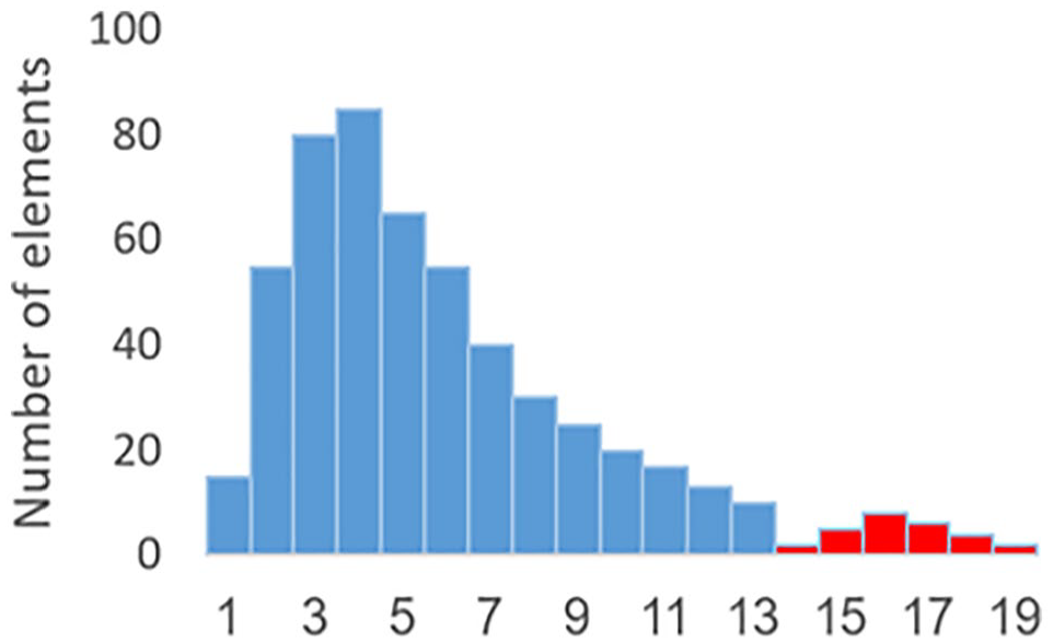
Illustration of rule 1.
In mathematical terms, the rule 1 can be described as follows


where
For the rule 2, we compare the local maximum (the peak cluster) of the smaller group (clusters 14 through 19 in Figure 9) to the last cluster of the larger, adjacent group, located right before the local minimum that separates the 2 groups (cluster 13 in Figure 9). If the cluster of the larger data group next to the local minimum contains more data elements than the maximum cluster of the smaller group, then we treat the smaller group as part of the larger group. In other words, we consider the smaller group being a result of batch effect (see Figure 9, where cluster 13 is larger than cluster 16).

Illustration of the rule 2.
In mathematical terms, the rule 2 can be described as follows
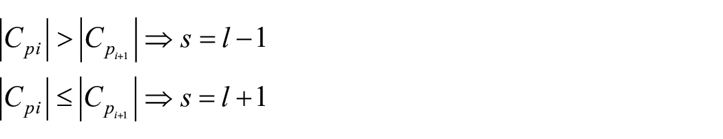
and

where
The 2 rules presented above should be treated as a preliminary work, and more research is needed to find additional heuristic rules to have greater confidence in evaluation process to decide, whether a separate group is truly a legitimate group, or an undesirable result of batch effect. Nevertheless, we have not found any reference in the literature that addresses this issue. The most popular methods for data normalization (to mitigate batch effect) do not address the possibility of 2 legitimate separate groups of data points. Normalization methods based on conventional statistical methodology (eg, ComBat) very often assume normal distribution of the data points within each gene, or uniform distribution of the data across the genes. Such assumptions are definitely unrealistic, at least based on our data. Hence, forcing gene’s data to conform normal, or any other uniform distribution across genes, will certainly cause severe distortion of the data, thus negatively affecting the analysis that follows. Several studies, referenced in the related literature presented above, reached similar conclusions, based on other considerations.
Additional issue that must be addressed in the context of the grouping of data, is the need to determine the border between groups (denoted by

or

In other words, when following the downward trend, and there are at least 2 consecutive increases, then we consider the downward trend broken. The border between the 2 groups will be the smallest cluster between them: the cluster N (eg, cluster 14 in Figures 8 and 9). Note that in the case of clusters of equal height, we move to the next cluster without changing the count.
The procedure to normalize each one of the groups (legitimate groups based on heuristic rules 1 and 2) is the same as presented in the previous chapter. First, we find the point of reference (the center of gravity) for each one of the data groups, separately (see Figures 10 and 11). In other words, we are utilizing the same process as explained in the previous section, only instead of applying it to the whole data of a gene, we apply it to the data of a given sub-group of gene’s data, based on its boundaries. After finding the centers of gravity for each of the data groups, we calculate center of gravity of each batch the same way, as explained in the previous section. Then, we compute the distance between center of gravity of each batch to the centers of gravity of each one of the data groups. We select as the point of reference for normalizing a batch—the center of gravity of the group, where such distance is the shortest. Then, we recompute the data for that batch (perform normalization) as explained in the previous section. Figure 12 illustrates this process. The range of the values of a given batch is represented by a horizontal green bar in the upper part of the figure. Point C represents the Center of Batch Cluster Group (CBCG). It is visually obvious that it is closer to the center of gravity of the cluster group located on the right. Therefore, the point of reference of the right-hand group is selected for normalizing that batch. The value of data points of that batch will be recalculated according to the algorithm presented in the previous section, and the whole batch will move to the right.

Finding the center of gravity of the first group.

Finding the center of gravity of the second group.

Normalizing a given batch.
As will be demonstrated in the next section, normalized data still maintain the distinction of the different groups, in contrast to ComBat, which forces the data into 1 group.
Case Studies
The human peripheral mononuclear blood cell (PBMC) samples from multiple sclerosis patients treated in Multiple Sclerosis Center, Sheba Medical Center, Israel, were processed on Affymetrix HU-133A-2 microarrays (Santa Clara, CA) according to manufacturer protocol between 2006 and 2014. A total 216 samples from 216 distinct individuals, combined from 24 batches associated with working sets consisting of 6 to 11 samples of each were analyzed. For all selected samples, raw CEL files were adjusted for GC content, probe set summarized by median polish algorithm implemented in Partek software ( www.partek.com ) and applied for batch normalization using BECHA and ComBat algorithms.
Note
BECHA allows up to 20 clusters to be constructed. Of course, it is logical to expect that if there are too few data points, the results might be distorted due to numerous clusters being empty. Based on literature, there is no consensus among professionals researching clustering methods, what is the minimum amount of data points which would be sufficient for reliable clustering results. Of course, it is always preferable to have bigger data set. The whole idea of combining many batches into larger data set is to have bigger data. However, if someone wants to find out, what is the lowest limit for reliable results, the way to go is to perform sensitivity test (taking smaller and smaller data sets) and to observe, when results will start changing significantly, in comparison with larger data sets. However, this issue is outside the scope of this study and was not addressed in this article.
The visualization of batch-effects was performed by scatter plot as implemented in Partek software using all prob-sets represented on Affymetrix Inc. HU-133A-2 microarrays or only for probes associated with Eukaryotic Poly-A RNA Controls supplied in the GeneChip 3 IVT Express Kit. The last contains 4 exogenous, pre-mixed, polyadenylated prokaryotic samples (lys, phe, thr, and dap) that are spiked directly into RNA samples before target labeling. Their resultant signal intensities on GeneChip arrays serve as sensitive indicators of target preparation and the labeling reaction efficiency, independent of starting sample quality and served as an indicator of data set variations associated with batch effect.
The results demonstrate, that in raw expression data (Figure 13A), samples clustered according to specific batches, suggesting that working sets present significant contribution to batch effects. A visual inspection after applying the 2 different batch effect adjustment methods BECHA and ComBat (Figure 13B and C) demonstrates a clear removal of the majority of batch effect observed in the raw data. After ComBat adjustment, the clouds associated with different batches are fully overlapped (Figure 13D and F), but the form of clouds (distribution of samples) has been seriously changed. After BECHA adjustment (Figure 13D and E), the batch centers are also similar; however, the form of clouds changed are more precise and clouds resemble the original inter-batch point distribution, suggesting more accurate batch effect adjustment by BECHA.

Visualization of batch effect adjustment. The scatter plot illustrates the 3-dimentional clusters of samples after principal component analysis (PCA) utilizing expression of all HU-133A-2 array probs. Upper panel: (A)—raw data before normalization; (B)—after BECHA; (C)—after ComBat. Lower panel: The samples of each batch were colored by 2 standard deviations (from centroid) clouds; (D)—raw data before normalization; (E)—after BECHA; and (F)—after ComBat.
To exclude the additional sources of heterogeneity affecting our data set, we have performed the principal component analysis (PCA) utilizing only 63 probes that are associated with HU-133A-2 arrays Poly-A RNA controls (Figure 14A to F). Note, even presented PCA analysis is illustrative of what we have observed, that batch adjustment by BECHA is more accurate to preserve inter-batch point distribution. The last suggestion is even more demonstrative by single gene profiling. Figure 15 presents clusters of a single gene characterized by 1 clear group (center of gravity) before normalization (A), after BECHA (B) and ComBat (C) batch adjustment. Both BECHA and ComBat method had similar samples distribution according to clusters. Figure 15D presents the corresponding boxplots of expression of this gene according to each of 24 batches. Similarly, both BECHA and ComBat reduced variability among batches in the same manner. However, the completely different results of normalization were observed when we have referred to single genes with more than 1 center of gravity. The analysis of one of such genes (208612_at) is presented in Figure 16.

Visualization of batch effect adjustment. Scatter plot illustrates the 3-dimentional clusters of samples after Principal Component Analysis (PCA) utilizing expression of HU-133A-2 arrays Poly-A RNA controls. Upper panel: (A)—raw data before normalization; (B)—after BECHA; (C)—after ComBat. Lower panel: The samples of each batch were colored by 2 standard deviations (from centroid) clouds; (D)—raw data before normalization; and (E)—after BECHA; (F)—after ComBat.

Expression profiling of single gene with 1 peak (center of gravity). Upper panel represents distribution of transcriptional levels of 200625_s_at gene across 18 clusters in data set without normalization (A), after BECHA (B) and ComBat (C) adjustment. Lower panel (D) represents 75% interquartile range boxplots of 200625_s_at gene expression associated with each batch in data set before normalization and after BECHA and ComBat adjustment.
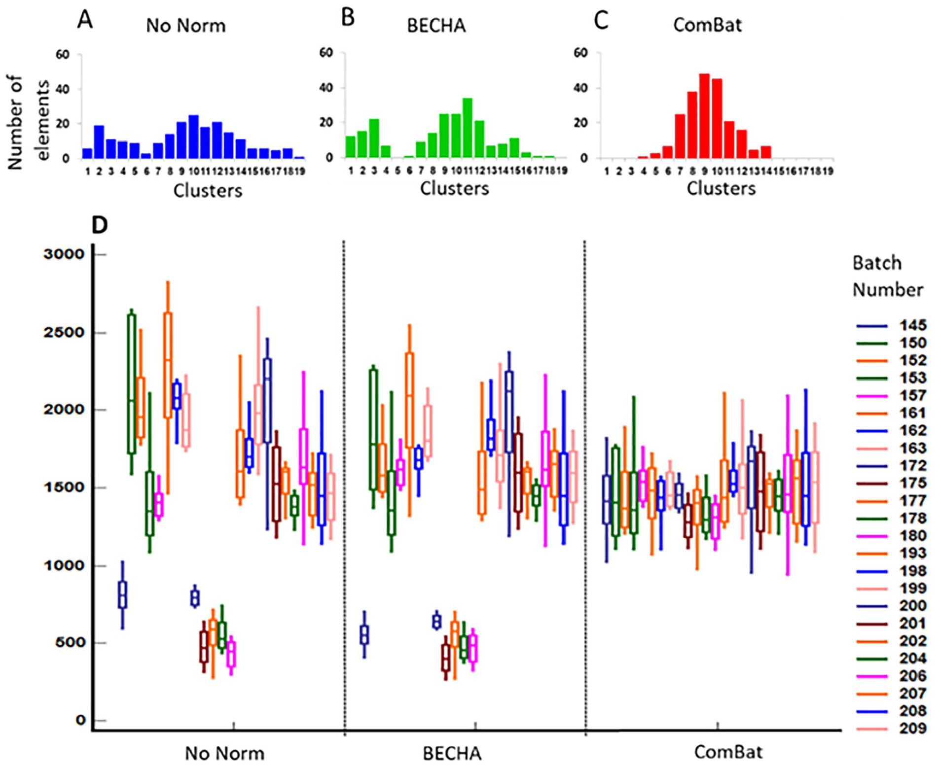
Expression profiling of single gene with 2 subgroups (centers of gravity). Upper panel represents distribution of transcriptional levels of 208612_at gene across 19 clusters in data set without normalization (A), after BECHA (B) and ComBat (C) adjustment. Lower panel (D) represents 75% interquartile range boxplots of 200625_s_at gene expression associated with each batch in data set before normalization (no norm) and after BECHA and ComBat adjustment.
As could be seen, the original 2-peak samples distribution across clusters were transformed into 1 peak by ComBat, while original 2 peak distribution was preserved by BECHA. The adjustment by ComBat greatly reduces batch effect in the cases of genes with the simple 1 center of gravity distribution. However, in more complicated situations characterized by distribution with more than 1 peak, batch adjustment by ComBat could distort original relations between samples that can lead to artificial changes in biological signals.
Note
The evaluation of the batch correction is challenging because the true batch effect influencing various measurements is unknown. One example of the attempt to evaluate normalization appears in Feng and Li, 33 where the authors examine the distribution of expression differentiation between 2 samples across all genes. However, the method is based on numerous assumptions and uses statistical methodology, which requires such assumptions. Based on the literature (section “The Batch Effect Correction Heuristic Algorithm (BECHA)”), all methods included are based on some assumptions regarding the distribution of the data. This makes all such performance tests subjectively dependent on the assumptions made. In contrast, our approach is based on assumption-independent Artificial Intelligence. As was stated above, there is no reliance in our method on a specific distribution of data, and therefore no assumptions were made regarding such distribution. Hence, the tests that are based on some underlying assumptions (regarding the distribution of data), are not applicable in our case. However, we did assure that the ratios among the values of the measurements belonging to the same batch remain the same after normalization, as they were before. We compared these results to ComBat, where the ratios among the values of measurements changed following the normalization, in comparison with the ratios before normalization. Maintaining the same ratios means that the normalization process did not affect the integrity of the data, which is not the case when data is forced into pre-assumed distribution. Therefore, from our perspective, this is the ultimate test. In addition, we performed numerous visual comparisons of the results based on our system vs the results of generated by ComBat, and we noticed that when the data distribution (of a gene) is close enough to normal, both methods generate similar outcomes. However, when the distribution of the data is further away from normal, then the distortions created by ComBat are clearly visible when observing the graphs. We cannot claim that our method is capable of entirely correcting data for batch effect. However, whatever correction is achieved, it is done without distorting the original batches. This is not the case of ComBat and other methods assuming specific data distribution.
Summary and Conclusions
In this study, we introduced an entirely new concept for normalization process designed to reduce batch effect. The method is conceptually simple. There are no assumptions made regarding the raw data distribution in contrast to the statistical methods (involving assumptions such as normal distribution, certain behavior of variance, error term, etc), and therefore, no additional biases are introduced when the behavior of the actual data substantially differs from the assumed one. It is true that BECHA is designed for large data sets, but because the process of normalization addressed in this study is designed in the first place for the purpose of creating large data sets, the problem of small data sets is not really an issue here. BECHA is intuitive, and the consequences of its applications are easy to understand. The ratios among the values of data elements within each batch remain the same before and after normalization, thus maintaining the integrity of the data.
The case study presented examples of batch effect normalization, based on several samples of multiple sclerosis patients. The results were compared with ComBat, thus demonstrating the advantages of BECHA.
Footnotes
Appendix
Let
Acknowledgements
Not applicable.
Funding:
The author(s) received no financial support for the research, authorship, and/or publication of this article.
Declaration Of Conflicting Interests:
The author(s) declared no potential conflicts of interest with respect to the research, authorship, and/or publication of this article.
Author Contributions
AY and ES have made substantial contributions to the conception, design of the work, and development of new normalization algorithm; MS made substantial contributions to the acquisition, analysis, and the creation of new software used in the work; and MG contributed to the clinical application and interpretation of data. All authors have drafted and substantively revised the manuscript and all authors read and approved the final manuscript.
Consent for Publication
Not applicable.
Ethics Approval and Consent to Participate
The study was approved by Sheba Institutional Review Board, and signed informed consent was obtained from all enrolled participants and all methods were performed in accordance with the relevant guidelines and regulations.