Sage Journals: Discover world-class research

Abstract

Small ribonucleic acid (sRNA) sequences are 50–500 nucleotide long, noncoding RNA (ncRNA) sequences that play an important role in regulating transcription and translation within a bacterial cell. As such, identifying sRNA sequences within an organism’s genome is essential to understand the impact of the RNA molecules on cellular processes. Recently, numerous machine learning models have been applied to predict sRNAs within bacterial genomes. In this study, we considered the sRNA prediction as an imbalanced binary classification problem to distinguish minor positive sRNAs from major negative ones within imbalanced data and then performed a comparative study with six learning algorithms and seven assessment metrics. First, we collected numerical feature groups extracted from known sRNAs previously identified in Salmonella typhimurium LT2 (SLT2) and Escherichia coli K12 (E. coli K12) genomes. Second, as a preliminary study, we characterized the sRNA-size distribution with the conformity test for Benford’s law. Third, we applied six traditional classification algorithms to sRNA features and assessed classification performance with seven metrics, varying positive-to-negative instance ratios, and utilizing stratified 10-fold cross-validation. We revisited important individual features and feature groups and found that classification with combined features perform better than with either an individual feature or a single feature group in terms of Area Under Precision-Recall curve (AUPR). We reconfirmed that AUPR properly measures classification performance on imbalanced data with varying imbalance ratios, which is consistent with previous studies on classification metrics for imbalanced data. Overall, eXtreme Gradient Boosting (XGBoost), even without exploiting optimal hyperparameter values, performed better than the other five algorithms with specific optimal parameter settings. As a future work, we plan to extend XGBoost further to a large amount of published sRNAs in bacterial genomes and compare its classification performance with recent machine learning models’ performance.

Keywords

sRNA accuracy paradox imbalance data machine learning AdaBoost XGBoost sRNA prediction

Introduction

Small or noncoding ribonucleic acids (sRNAs or ncRNAs) play a major role in the regulation of several molecular processes within a bacterial cell. They are usually between 50 and 500 nucleotides long and can be classified into two major categories: cis-encoded (or antisense), and trans-encoded sRNAs.¹ The basis of this classification relies on the location of the sRNA sequence within DNA regarding its corresponding messenger RNA (mRNA) target, as well as the base-pair interaction between sRNA and mRNA transcript.² As sRNAs are transcribed from DNA strands but do not undergo translation, they are usually located in non-coding regions of DNA (also referred to as intergenic regions).³ Cis-encoded sRNAs can be found in regions of the genome that overlap with the sequence of their mRNA target, resulting in extensive and complete complementarity of the sRNA-mRNA hybrid.⁴ Trans-encoded sRNAs are found in regions separate from their target mRNA genes; thus, they resemble minimal, but are with effective complementarity to their targets.⁵ In addition, the nonspecific binding of sRNA molecules allows for multiple targets to be accessed by a single trans-encoded sRNA.⁶

The binding of sRNAs to mRNA transcripts plays an important role in regulating transcriptional and/or translational processes. A majority of sRNAs, both cis- and trans-encoded, regulate their respective targets in a negative manner through different mechanisms that interfere with translational machinery.⁷ Small RNAs, such as RyhB⁸ and CsrA⁹ in Escherichia coli, bind to important translation initiation sequences and block translational machinery from recognizing the mRNA transcript. Other sRNAs, such as SgrS in Escherichia coli and Salmonella strains,¹⁰ bind to regions further upstream the translation initiation sites, covering sequences required for promoting translation. Positive effects of sRNAs on translation have also been identified, where sRNAs can bind and alter the structure of a mRNA to be easily accessed by translational machinery.¹¹ In addition, sRNAs can have an impact on the transcriptional activity of a target gene by inhibiting proper termination of a pre-determined transcript.¹²

The recognition of sRNAs in bacteria is useful in understanding the way bacteria regulate gene expression under various environmental conditions. Previous research has revealed the value of sRNAs in regulating gene expression when a bacterium is placed under stress.¹³ Certain stressors, such as nutrient deficiency,^14,15 cell envelope stress,^16-18 and oxidative stress,^19-22 are a few examples where sRNAs are found to be most prevalent in bacterial regulatory systems. In addition, sRNAs play a big role in regulating genes responsible for virulency in pathogenic microbes.²³ Aside from sRNAs being present under stress and virulence, these regulatory molecules have been shown to influence everyday cellular metabolism at primary and secondary levels in different bacterial species.²⁴ While sRNA identification has been thoroughly examined in bacterial model organisms such as Escherichia coli and Salmonella enterica,²⁵ a large majority of bacterial species have yet to be explored for the presence of regulatory sRNAs. The ability to efficiently recognize sRNA sequences in different bacterial genomes can assist in conducting experiments to understand how these regulatory molecules impact cellular processes. Furthermore, identifying sRNAs across different groups of bacteria can shine a light on the evolutionary history of bacterial strains.⁷

To verify the presence of any potential sRNA sequence, various laboratory techniques such as microarrays, Northern blotting, and size-selective RNA sequencing are necessary.²⁶ This verification is necessary to correctly determine the presence of a sRNA in vivo. In addition, other laboratory experimentations are required to validate the mechanisms by which an sRNA interacts with its respective target(s).²⁷ However, such wet-lab experiments are tedious, time-consuming, and costly for laboratory researchers. To maximize efficiency for experimental design, it is crucial to utilize cost-efficient methods of accurately predicting novel sRNA sequences and their potential mRNA targets. Therefore, it is beneficial to employ computational approaches that can streamline experimental verification processes for detecting sRNAs and their interactions with targets.

Recently, various machine learning-based approaches have been applied to predict sRNAs in any given bacterial genome. Grüll et al²⁸ identified putative sRNAs in Rhodobacter capsulatus by the sequence similarity to sRNAs in a sRNA collection and represented each putative sRNA (or a random genomic sequence) as a group of seven numerical attributes that biologically characterize the putative sRNAs’ distinct genomic contexts and characteristics. Then, using the logistic regression model, they obtained the likelihood of the putative sRNAs to be a potential candidate for sRNA. Tang et al²⁹ integrated various sequence-derived 17 feature groups and built two ensemble learning models, the Weighted Average Ensemble Method (WAEM) and the Neural Network Ensemble Method (NNEM), for the sRNA prediction. In another study, Eppenhof and Peña-Castillo³⁰ adopted seven biological features by Grüll et al,²⁸ employed five traditional machine learning algorithms (including Logistic Regression (LR),³¹ Multi-Layer Perceptron (MLP),³² Adaptive Boosting (AB),³³ Gradient Boosting (GB),³⁴ and Random Forest (RF)),³⁵ and assessed the performance of the algorithms on benchmark datasets.

Motivated by the encouraging result from the related research work^28-30 that utilized varied individual feature sets along with several machine learning algorithms, we aim to leverage the classification performance by identifying and combining best features, varying positive to negative data ratios, utilizing another decision tree-based ensemble learning algorithm, eXtreme Gradient Boosting (XGBoost),³⁶ and employing seven evaluation metrics. As in the existent studies,^29,30 we make use of the Salmonella typhimurium LT2 (SLT2) and the Escherichia coli K12 (E. coli K12) datasets. Specifically, we concatenated seven numerical attributes (or features) published work by Eppenhof and Peña-Castillo³⁰ and let G1 denote the group of seven attributes. In addition, we extracted 2,222 sequence-derived features by utilizing the python package repDNA³⁷ and let G2—G15 denote each of 14 sets of attributes, respectively. Characteristics of two previous research that motivated the current study are summarized in Table 1 and details of 15 feature groups are described in Table 2.

Table 1.

Characteristics of related research and this study.

Source	Tang et al²⁹	Eppenhof and Peña-Castillo³⁰	This study
Algorithms	Weighted Average Ensemble Method (WAEM) and Neural Network Ensemble Method (NNEM)	Logistic Regression (LR), Multilayer Perceptron (MP or MLP), Random Forest (RF), Adaptive Boosting (AB, or AdaBoost), and Gradient Boosting (GB)	Logistic Regression (LR), Multilayer Perceptron (MLP), Random Forest (RF), Adaptive Boosting (AB), Gradient Boosting (GB), and eXtreme Gradient Boosting (XGB, or XGBoost)
Training Datasets	Salmonella typhimurium LT2	Rhodobacter capsulatus Streptococcus pyogenes, Salmonella enterica, and combined	Salmonella typhimurium LT2 and Escherichia coli K12
Test Datasets	Salmonella typhimurium LT2	Rhodobacter capsulatus, Streptococcus pyogenes, Salmonella enterica, Escherichia coli K12, and Mycobacterium tuberculosis	Salmonella typhimurium LT2 and Escherichia coli K12
Features	2,222 sequence-derived features	7 biological features	7 biological features and 2,222 sequence-derived features
Feature Groups	G2—G15	G1	G1—G15
Positive to Negative Data Ratio	1-to-1, 1-to-2, 1-to-3, 1-to-4, and 1-to-5	1-to-3 for training data, and either 1-to-37 or 1-to-10 for test data	1-to-1, 1-to-2, 1-to-3, 1-to-4, 1-to-5, 1-to-6, 1-to-7, 1-to-8, 1-to-9, and 1-to-10
Metrices	Accuracy and Area Under the ROC curve (AUROC, or AUC)	AUROC and Area Under the Precision Recall curve (AUPR)	Accuracy, Balanced Accuracy, Precision, Recall, F1-measure, AUROC, and AUPR
Validation	5–fold cross-validation	Random 80% – 20% split for each of 5 training runs	Stratified k–fold cross-validation with k = 5 and k = 10

Abbreviations: AB, Adaptive Boosting; AUPR, Area Under the Precision Recall curve; AUROC, Area Under the ROC curve; GB, Gradient Boosting; LR, Logistic Regression; MLP, Multilayer Perceptron; NNEM, Neural Network Ensemble Method; RF, Random Forest; WAEM, Weighted Average Ensemble Method; XGB, eXtreme Gradient Boosting.

Table 2.

Feature groups publicly available and used for this study.

Abbreviation	Feature group	Number of features	Reference
G1	Biological features	7	Eppenhof & Peña-Castillo³⁰
G2 (F1)	1-mer	4	Tang et al²⁹
G3 (F2)	2-mer	16
G4 (F3)	3-mer	64
G5 (F4)	4-mer	256
G6 (F5)	5-mer	1,024
G7 (F9)	1-RCkmer	2
G8 (F10)	2-RCkmer	10
G9 (F11)	3-RCkmer	32
G10 (F12)	4-RCkmer	136
G11 (F13)	5-RCkmer	512
G12 (F14)	PCPseDNC	17
G13 (F15)	PCPseTNC	65
G14 (F16)	SCPseDNC	18
G15 (F17)	SCPseTNC	66

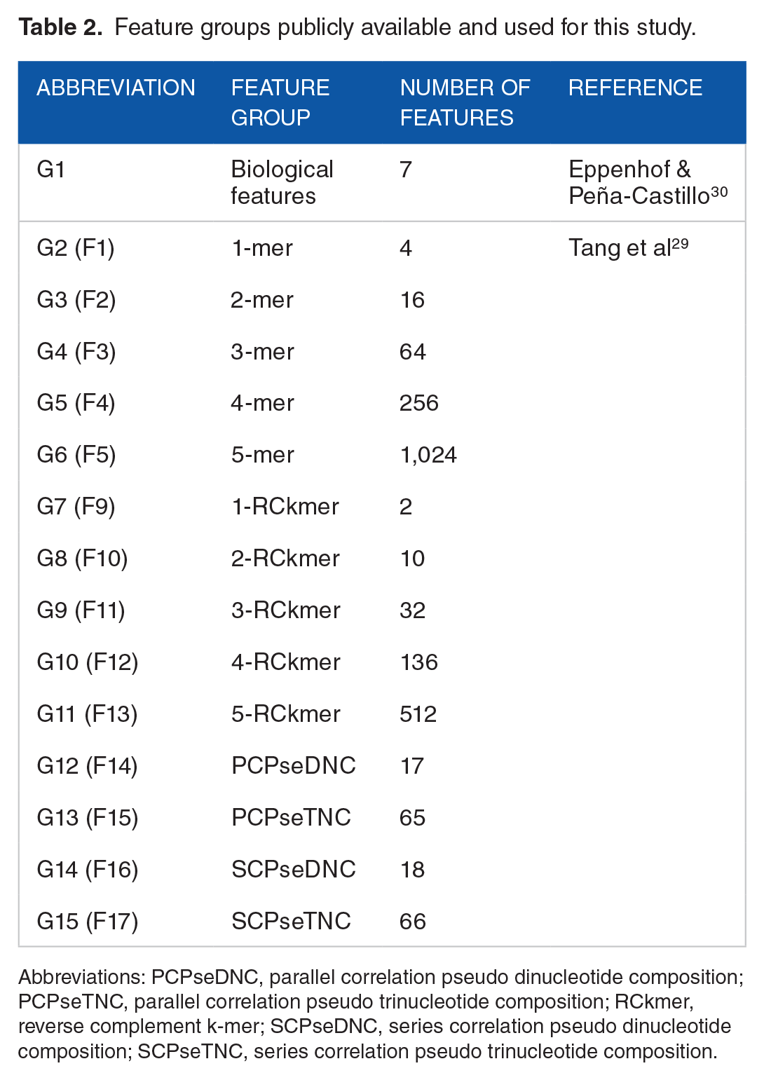
Abbreviations: PCPseDNC, parallel correlation pseudo dinucleotide composition; PCPseTNC, parallel correlation pseudo trinucleotide composition; RCkmer, reverse complement k-mer; SCPseDNC, series correlation pseudo dinucleotide composition; SCPseTNC, series correlation pseudo trinucleotide composition.

As in Table 1, the sRNA datasets are imbalanced as the class of interest (i.e. positive, or minority class) is relatively rare, compared to the other class (i.e. negative, or major classes). One of the most common challenges while trying to classify imbalanced data is that the classifier can be heavily biased toward the majority negative class.^38,39 To illustrate the challenge in evaluating classification performance on imbalanced data, let us consider that accuracy, the most often used metric that measures the fraction of correctly classified instances, is employed to evaluate the classification performance with the skewed dataset, whose positive to negative data ratio is 1-to-10. As the minority class makes 10% of the instances while the majority occupies the remaining 90% of the instances, one can obtain an accuracy of 0.9 (i.e. 90%) by simply predicting all instances as the majority class. The minority class has very little impact on the accuracy as compared to that of the majority class. An accuracy of 0.9 (i.e. 90%) seems high; however, it can be misleading as it has no predictive power on the minority class. This is called accuracy paradox, which states that predictive model with a given level of accuracy may have greater predictive power than models with higher accuracy.⁴⁰ Accuracy paradox has been identified and discussed in real-life applications with skewed or imbalanced datasets.^41-43

In this research, we interpreted the prediction of sRNAs as a supervised learning with imbalanced data. Then, we aimed to comparatively assess three questions on the learning problem: what numerical features extracted from sRNAs are suitable for learning; what traditional classification algorithms are robust to various feature groups, and what evaluation metrics are appropriate for measuring the performance of learning from imbalanced data, using published data and well-studied metrics for classification performance.

Materials and Methods

Datasets

To effectively compare our classifier performance against currently existing predictive models, we utilized the same training and testing datasets originally generated and used by Tang et al²⁹ and Eppenhof and Peña-Castillo.³⁰ Specifically, we used data from the Salmonella typhimurium LT2 (SLT2) genome and the Escherichia coli K12 (E. coli K12) genome. Browser Extensible Data (BED) files from the study by Eppenhof and Peña-Castillo³⁰ contain information about all experimentally verified sRNAs in SLT2, such as genomic coordinates, length, and strand in which the sRNAs are located. First, we processed the BED files and extracted the respective sRNA sequences from the genome. For sequences located on the negative strand, we generated the reverse complement of the equivalent sequence on the positive strand. After compiling these sequences, we stored this list of verified sRNAs as a positive dataset.

An ideal negative dataset is one that is clearly separable from the positive dataset. We used the dataset used by Eppenhof and Peña-Castillo.³⁰ They generated the negative instances from the coding regions of DNA that are characteristically distinct from the intergenic/non-coding sRNA sequences and then they removed any negative data that overlapped with positive sRNA sequences to ensure that this negative dataset would perform optimally. The remaining dataset had approximately 10 times as many negative instances as positive instances. Therefore, we assessed the performances of learning models with varying positive-to-negative instance ratios to consider all the spectrum of the data ratios, where 1-to-1 ratio is balanced, and the others are imbalanced.

The two specific datasets were publicly available for SLT2. The first STL2 dataset is the fixed training-test split with a total of 1239 instances, including 361 (90(+) and 271(-)) training instances and 878 (23(+) and 855(-) test instances and the other one is the whole positive-negative split with the total of 1986 (182(+) and 1804(-)) instances, where plus (+) and minus (-) symbols denote positive and negative sRNAs, respectively. We used the fixed training-test data to compare the performance between the training-test split and the k-fold cross-validation. The fixed training-test dataset with the reduced number of instances, selected from the whole positive-negative split, was originally used by Tang et al²⁹ and later by Eppenhof and Peña-Castillo.³⁰ The whole positive-negative split is the second STL2 dataset and it is available in the BED files by Eppenhof and Peña-Castillo.³⁰ The whole positive-negative split dataset with 1986 instances of SLT2 was used to assess the feature importance and feature group importance. E. coli K12 dataset has only the positive-negative split with the total of 1369 (125(+) and 1244(-)) instances. As the positive-to-negative instance ratio is approximately 1-to-10, the positive-negative split datasets were used to assess how the different data ratios affect the classification performance.

Sequence-derived feature sets

From the positive and negative sRNAs in SLT2 and E. coli K12, we extracted the total of 15 groups of distinct numerical features, which have been already studied in the related approaches.^28-30 Using a Python pipeline tool, sRNACharP³⁰ (available at https://github.com/BioinformaticsLabAtMUN/sRNACharP), we obtained numerical features that characterize various biochemical aspects of each sequence. Specifically, the tool generates the group (denoted as G1) of seven features, including free energy of the sRNA secondary structure (f1), distance to the closest promoter upstream of the sRNA (f2), distance to the closest Rho-independent terminator (f3), distance to the closest left Open Reading Frame (ORF) (f4), Boolean value (0 or 1) indicating if sRNA is on the same strand as left ORF (f5), distance to the closest right ORF (f6), and Boolean value indicating if sRNA is on the same strand as right ORF.

In addition to above seven biological features extracted, utilizing another python package, repDNA³⁷ (available at http://bioinformatics.hitsz.edu.cn/repDNA/), we converted each input sequence into a list of L1-norm normalized values relating to different sequence-derived characteristics. Tang et al²⁹ extracted a total of 17 distinct numerical feature groups (indexed from F1 to F17) from the 182 experimentally verified sRNAs in SLT2 for their study. However, using repDNA, we were able to generate only a total of the 14 feature groups as follows: K-mer (with k ranging from 1 to 5) (G2—G6), reverse compliment k-mer (with k ranging from 1 to 5) (G7—G11), parallel correlation pseudo dinucleotide composition (G12), parallel correlation pseudo trinucleotide composition (G13), series correlation pseudo dinucleotide composition (G14), and series correlation pseudo trinucleotide composition (G15). Specifically, mismatch profile group,³⁰ including the three feature sets F5—F7, was not used for our study. For the reference, the indices of our feature groups and the matched feature groups by Tang et al²⁹ are given in Table 2.

The k-mer features represent the frequency of the unique k-sized subsequences in each given sequence. For example, 1-mer would return the four frequency values, corresponding to the four mononucleotides (i.e. adenosine (A), cytosine (C), guanine (G), and thymine (T)). For 2-mer, it would return 16 frequency values for the 16 dinucleotides, respectively. The reverse compliment k-mer functions act in a similar fashion; however, it removes redundancies based on sub-sequences that are the reverse complement of each other. The four pseudo-nucleotide composition features return the frequencies of different dinucleotide and trinucleotide sequences relating to specific physiochemical properties. A more in-depth explanation can be found in the repDNA manual. The entire feature set collected for this study consists of 2,229 features over 15 feature groups, which include both G1 with seven features and G2—G15 with 2,222 features, as summarized in Table 2.

Tools and software

The entire experiment was performed on Google Colab, a collaborative Python Integrated Development Environment (IDE). repDNA³⁷ package and sRNACharP³⁰ pipeline tool were utilized to extract numerical sequence-derived features that characterize various biochemical aspects of each RNA sequence for our study. Scikit-learn (sklearn) (ver. 1.0)⁴⁴ for the implementation of the six machine learning algorithms in Python: Logistic Regression (LR) (LogisticRegression()), Multi-Layer Perceptron (MP or MLP) (MLPClassifier()), Random Forest (RF) (RandomForestClassifier()), Adaptive Boosting (AB or AdaBoost) (AdaBoostClassifier()), Gradient Boosting (GB) (GradientBoostingClassifier()), and eXtreme Gradient Boosting (XGB or XGBoost) (XGBClassifier()), which is the scikit-learn wrapper class for the XGBoost library.³⁶ Finally, all figures based on the performance metrics were generated through MATLAB (ver. R2021a).

Hyperparameter values for classification algorithms

Eppenhof and Peña-Castillo³⁰ used five traditional classification algorithms, including Logistic Regression (LR), Multi-Layer Perceptron (MP or MLP), Adaptive Boosting (AB or AdaBoost), Gradient Boosting (GB),³⁴ and Random Forest (RF), with specific hyperparameter values to fit each model. They obtained best parameter values for each algorithm in terms of maximizing the average area under the ROC curve (AUROC or AUC) with leave-one-out cross-validation (LOO CV) on the training data. Finding best hyperparameters and values that optimize each learning algorithm and specific datasets is another challenging research problem. Therefore, we used the identical hyperparameters and values originally found by Eppenhof and Peña-Castillo.³⁰ They performed leave-one-out cross-validation (LOO CV) on the training data as depicted in Figure 2 of Eppenhof and Peña-Castillo³⁰ and identified best parameter values per each classifier that maximized the average area under the ROC curve (AUROC).

Specifically, for LR (LogisticRegression()), the maximum likelihood and the balanced mode are used to adjust class weights inversely proportional to class frequencies in the input data (i.e. class_weight ='balanced'). For MLP (MLPClassifier()), the standard backpropagation with the logistic sigmoid activation function, a hidden layer with 400 neurons, the maximum iteration of 200, the quasi-Newton optimizer, the L2 penalty of 0.0001, a constant running rate, the initial learning late with 0.9, the exponent for inverse scaling learning rate with 0.8 are used (i.e. hidden_layer_sizes = (400), activation ='logistic', solver ='lbfgs', max_iter = 200, alpha = 0.0001, verbose = 0, learning_rate ='constant', learning_rate_init = 0.9, power_t = 0.8). For AB (AdaBoostClassifier()), a random forest (RF) (RandomForestClassifier()) classifier with 100 decision trees (estimators) and a maximum depth of 1 is used. (i.e. n_jobs = 3, n_estimators = 100, max_depth = 1). For GB (GradientBoostingClassifier()), a total of 50 decision trees (estimators) with a maximum depth of 15, maximum features of 7, minimum samples (at a leaf node) of 5, stochastic gradient boosting with subsampling of 0.9 are used (i.e. n_estimators = 50, max_depth = 15, max_features = 7, min_samples_leaf = 5, verbose = 1, subsample = 0.90). For RF (RandomForestClassifier()), the maxim number of decision trees (estimators) of 400 and the maximum number of features (for the best split in a node) of 2 are set (i.e. n_jobs = 3, n_estimators = 400, max_features = 2).

EXtreme Gradient Boosting (XGBoost, or XGB) is the one of the latest evolutions of the traditional decision tree algorithm.³⁶ As it is known to optimize the performance of existing decision tree-based models, we employed XGBoost to see if it further improves upon the results of the existing studies. Particularly, we executed XGBoost (XGBoostClassifier()) with no search for best hyperparameter values; thus, the baseline experimental performance of XGBoost reported here can be improved further with a grid search of hyperparameter values if needed.

Evaluation metrics

Confusion matrix summarizes a model’s capability for generating true positives (TP), true negatives (TN), false positives (FP), and false negatives (FN), where TP is the number of positive instances correctly classified as positive, TN is the number of negative instances correctly classified as negative, FP is the number of negative instances incorrectly classified as positive, and FN is the number of positive instances incorrectly classified as negative.

Evaluation metrics can be defined directly from a confusion matrix as follows.

Accuracy, defined as (TP + TN)/(TP + FP + TN + FN), is the most often used metric that measures the fraction of correctly classified instances. As discussed previously, accuracy is not an appropriate evaluation metric for imbalanced data since it does not distinguish between the numbers of correctly classified examples of different classes. Specifically, it ignores two different types of errors, false positive (i.e. Type I error) and false negative (i.e. Type II error).

Precision (also known as positive predictive value), defined as TP/(TP + FP), measures how often an instance was predicted as positive that is originally known positive.

Recall (also known as TP rate or sensitivity), defined as TP/(TP + FN), measures how many of positive instances in a dataset were detected. Note that specificity (also known as true negative rate or 1—FP rate), defined as TN/(TN + FP), measures how many of negative instances in a dataset were detected. In evaluation performance for imbalanced data, it is desirable to improve recall without hurting precision. However, this goal is often conflicting, as we try to increase the TP for the minority class, the FP is also often increased, which results in reduced precision. Also, precision can be biased by very unbalanced class priors in the test sets.

More advanced evaluation metrics have been proposed to remedy for accuracy paradox for imbalanced data as follows.

The first alternative is balanced accuracy,^45,46 which is designed to avoid inflated performance estimates on imbalanced data. It is defined as the macro average of recall scores per class (or equivalently, raw accuracy where each sample is weighted according to the inverse prevalence of its true class). Notice that for a balanced dataset, balanced accuracy score is equal to accuracy and for a binary case, it is equivalent to the arithmetic mean of sensitivity

(TPN) and specificity (TNR) (= ½ (TP/(TP + FN) + TN/((TN + FP)). Therefore, different from accuracy, balanced accuracy computes the average of the percentage of positive class instances correctly classified and the percentage of negative class instances correctly classified, taking into consideration to give an equal weight to the relative proportions for the two classes.

The second alternative is F1 score (also known as balanced F-score or F-measure), a special case of the general equation Fβ-measure,⁴⁷ defined as Fβ = (1 + β2)*(precision*recall) / ((β 2 *precision) + recall). Fβ-measure is a family of metrics that can measure trade-offs between precision and recall by outputting a single value that reflects the goodness of a classifier in the presence of rare classes. With a higher β, the more weight or emphasis is on recall over precision. Specifically, F1 score (i.e. β = 1) is a harmonic mean of precision and recall; thus, both precision and recall are equally weighted.

The third alternative is Area Under the Receiver Operating Characteristic curve (AUROC)⁴⁸ (also known as area under the curve (AUC)), which is a numerical representation of a binary classifier’s ability to differentiate between positive and negative inputs. AUROC is based on a ROC curve, which is plotted to visualize the classification performance between TP rate (also known as Recall or sensitivity) at the y-axis and FP rate (= 1–specificity = 1–TN/(TN + FP) = FP/(FP + TN)) at all classification thresholds. Therefore, ROC curves represent the trade-off between different TP rates and FP rates.

The fourth alterative metric to better understand the trade-offs between precision and recall for imbalanced data is Area Under the Precision-Recall curve (AUPR),^49,50 which is another numerical representation of a binary classifier’s ability to differentiate between positive and negative inputs. AUPR is based on a PR curve like AUROC on a ROC curve. Notice that while in a ROC curve, FP rate (also as recall) is at x-axis and TP rate at y-axis, in PR curves, recall is at x-axis and precision at y-axis. Previous research suggests that AUPR provide more robust and better performance metrics for imbalanced data.^49-51 Furthermore, AUPR is considered a better discriminator of classification performance than AUROC.

Throughout the empirical study, we aimed to gain insight on characteristics of target datasets, importance of numerical features extracted from sRNAs, effectiveness of seven metrics on imbalanced class distributions, and effect of positive-to-negative data ratio (from 1-to-1 to 1-to-10). The predictive power of all six classification models were assessed by seven metrics over k-fold cross-validation.⁵² Both 5-fold cross-validation (5-fold CV) and 10-fold cross-validation (10-fold CV) were performed, where each dataset was split into k equal-sized folds using the stratified sampling and all the performance metrics were macro-averaged over the k-fold iterations for k = 5 and 10, respectively. Particularly, stratified k-fold cross-validation is employed to unbiasedly learn from imbalanced class distributions. Note that the range of all seven metrics used in this study is [0, 1] with no unit, which can be interpreted as percentages; however, for simplicity, the real values in [0, 1] are used as they are. Also, mean and standard deviation (std) of metric values from k-fold cross-validation are denoted by (mean±std) for reference.

Results and Discussion

Conformity test for Benford’s law on lengths of sRNAs in Salmonella typhimurium LT2 (SLT2) and Escherichia coli K12 (E. coli K12)

In 1881, Simon Newcomb⁵³ originally found that numbers more frequently begin with smaller digits than with larger digits and the probability of each following digit at the most significant position progressively decreases. Later in 1938, Frank Benford⁵⁴ rediscovered and extended it with extensive testing and analysis with a wide variety of observations of natural numbers in numerous real-life datasets. Therefore, it is known as a first digit law, leading digit phenomenon, or Benford-Newcomb phenomenon. According to Benford’s law, there are expected frequencies of digits in a randomly generated dataset. Specifically, the leading digits of numbers in a naturally occurring set of numbers do not occur with uniform probability; thus, it has become one of the most popular digital analytical techniques for numerous applications such as accounting, economies, natural sciences, engineering, medicines, to name a few. Some known criteria for data to obey Benford’s law include that the quantities are geometrically distributed, the mean is greater than the median, and data span several orders of magnitude.^55-57

Our focus is to examine whether sRNA lengths conform the leading digit phenomenon as observed in various natural numbers in real-life applications. sRNAs maintain variation under different selection pressures in genomes. Although primary sequence variation is originated by random mutation, mutated sequences coevolve with their corresponding target gene sequences, resulting in optimal gene regulating mechanisms. Therefore, sRNA lengths may not comply a leading digit phenomenon of the Benford’s law. If there are deviations from Benford’s law, we may conclude that sRNAs do not evolve through random mutation alone. Instead, specific nucleotide locations are differentially constrained due to biological adaptation to complementary sequences in target genes.

The summary statistics of the lengths of the known sRNAs of the two datasets are as follows: SLT2 (count = 182, mean = 206.98, std = 184.20, median = 145.50, min = 45, Q1= 95.25, Q2= 145.50, Q3= 258.50, max = 1,236) and E. coli K12 (count = 125, mean = 156.63, std = 148.56, median = 113.0, min = 40, Q1 = 82, Q2 = 113, Q3 = 184, and max = 1454), where Q1, Q2, and Q3 stand for first, second, and third quartile, respectively. The length distribution of sRNAs in SLT2 can be found in Figure 1 by Tang et al.²⁹ Other detailed stochastic properties or characteristics of the sRNAs are yet to be analyzed, but we noticed that the mean of the lengths of the known sRNAs is greater than the corresponding median as well as the grouped length distribution in Figure 1 by Tang et al²⁹ is skewed. Therefore, to further characterize the sRNAs, we investigated whether there might exist any regularities in the sRNA-size distribution, using the conformity test for Benford’s law.^53-55

Figure 1.

The first 1 digit test for the lengths of sRNAs in SLT2 (top) and E. coli K12 (bottom). Each graph depicts distribution of first 1 digits (in bar graphs), region of confidence level, and entries with significant positive or negative deviations (in orange bar graphs). The region of 95% confidence interval is shown in the left graph and the region of 99.9% confidence interval in the right graph, respectively. The graphs and results are generated using the python package Benford_py (available at https://github.com/milcent/benford_py).

The first 1 digits (F1Ds) of the sRNA size of SLT2 do not conform to Benford’s law as the Mean Absolute Deviation (MAD) of 0.035434 is greater than the critical value of 0.015000. For the 95% confidence interval, it fails both Kolmogorov-Smirnov (K-S) test (0.111058 > 0.100662 (critical value)) and Chi-square test (24.564711 > 15.507000 (critical value)). Particularly, F1D 1 is with significant positive deviation (0.30103 (expected), 0.412088 (observed), and 3.185464 (z-score)) and F1D 4 is with significant negative deviation (0.096910 (expected), 0.038462 (observed), and 2.540099 (z-score)). However, for the 99.9% confidence interval, it passes both K-S test (0.111058 < 0.183089 (critical value)) and Chi-square test (24.564711 < 37.332000 (critical value)).

The F1Ds of the sRNA size of E. coli K12 do not conform to Benford’s law, either. The MAD of 0.048015 is greater than critical value of 0.015000. For the 95% confidence interval, it passes K-S test (0.109098 < 0.121463 (critical value)), but it fails Chi-square test (29.896199 > 15.507000 (critical value)). Particularly, the two entries are with significant positive deviations: F1D 8 (0.051153 (expected), 0.112 (observed), and 2.884925 (z-score)) and F1D 1 (0.301030 (expected), 0.408 (observed), and 2.509756 (z-score)) and two entries are with significant negative deviations: F1D 4 (0.096910 (expected), 0.032 (observed), and 2.301939 (z-score)) and F1D 2 (0.176091 (expected), 0.096 (observed), and 2.233476 (z-score)). However, for the 99.9% confidence interval, it passes both K-S test (0.111058 < 0.183089 (critical value)) and Chi-square test (24.564711 > 37.332000 (critical value)).

Even though the F1Ds of the lengths of the known sRNAs in SLT2 and E. coli K12 have the cases of nonconformity to Benford’s law in terms of MAD, both datasets have cases of passing the K-S test and the Chi-square test with the small number of instances as discussed above. Therefore, it might be too early to draw a conclusion. The deviations from Benford’s law might be attributed to the small subset (or sample) problem, lacking statistical power and representativeness, or the latent bias toward different dynamics of biological domains as discussed by Friar et al.⁵⁷

Classification with G1 feature group of fixed training-test split data of SLT2

We analyzed the learning models’ performance on the fixed G1 dataset published by Eppenhof and Peña-Castillo.³⁰ The dataset captures a unique set of seven biological features for sRNAs. First, these seven features are extracted for each instance (or sequence) in the fixed G1, which consists of the reduced set (i.e. the selected instances) from the full SLT2 data. Then, we assessed classification performance of six classification models (LR, MLP, AdaBoost, GB, RF, and XGBoost). The fixed training-testing split of G1 executed one time execution, while k-fold cross-validation (CV) performed k iterations. Eppenhof and Peña-Castillo³⁰ originally found the optimized hyper-parameter values for LR, MLP, AdaBoost, GB, and RF, that could maximize AUROC; thus, we used the optimized hyper-parameters for the five algorithms as they were. However, we did not exploit optimal parameter values for XGBoost in our study. We assessed the classification performance using both 5–fold CV and 10–fold CV as shown in Figure 2. We found that the difference of mean performance between 5–fold CV and 10–fold CV was not significant. For example, two-tailed t-test for two independent means at significant levelα = .01 for AUPR is as follows: LR (t(13) =-0.369, P = .726) with 5-fold CV (0.37 ± 0.04) and 10-fold CV (0.41 ± 0.17); MLP (t(13) = -0.845, P = .414) with 5-fold CV (0.62 ± 0.01) and 10-fold CV (0.67 ± 0.11); AdaBoost (t(13) = -0.341, P = .738) with 5-fold CV (0.82 ± 0.01) and 10-fold CV (0.84 ± 0.05); GB (t(13) = -0.186, P = .855) with 5-fold CV (0.79 ± 0.02) and 10-fold CV (0.80 ± 0.07); RF (t(13) = -0.314, P = 0.759) with 5-fold CV (0.80 ± 0.01) and 10-fold CV (0.82 ± 0.07); and XGBoost (t(13) = -0.875, P = 0.397) with 5-fold CV (0.82 ± 0.02) and 10-fold CV (0.85 ± 0.05). Therefore, we rather discuss the result with 10-fold CV in the remaining sections, unless otherwise specified.

Figure 2.

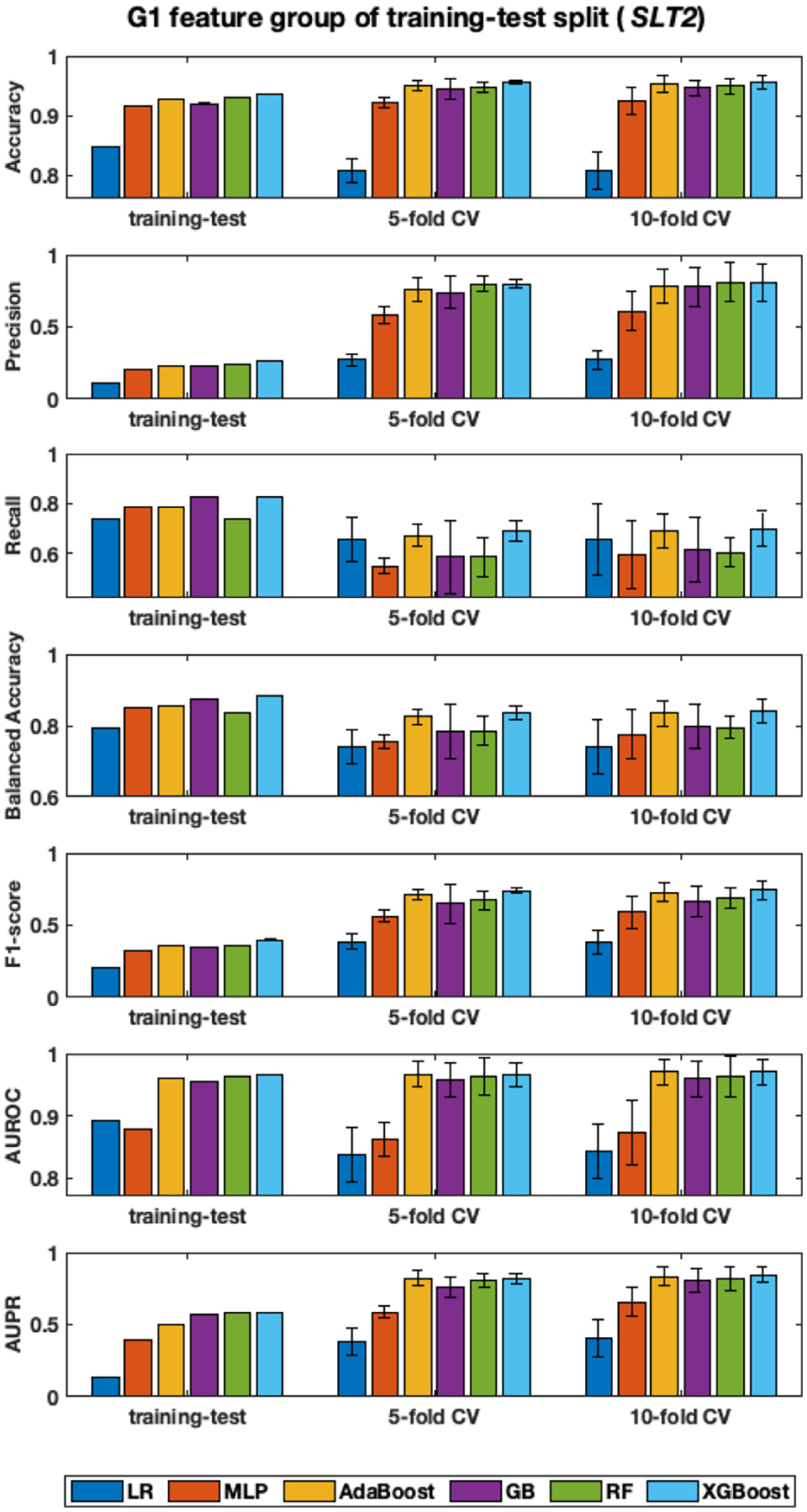
Classification performance on fixed training-test split of G1 feature group of sRNAs in SLT2. Each subplot shows classification performance of six classification algorithms, measured by one of seven metrics. The x-axis displays the tree groups of experiments, including the fixed (or published) training-test split, 5-fold CV, and 10-fold CV. The range of y-axis is adjusted to emphasize changes in values. Only single mean value is available for fixed training-test split, while both micro-average means and standard deviations are calculated over 5-/10-fold cross-validations.

In terms of accuracy, precision, and recall, it is ambiguous to rank the performance. However, the other four metrics clearly helps identify algorithms’ performance. Overall, LR and MLP performed poorly; GB and RF did reasonably better; and AdaBoost and XGBoost demonstrated best performance. As GB, RF, AdaBoost, and XGBoost are tree-based ensemble models, similar results could be expected in fact. It is important to note that XGBoost without optimized parameters performs roughly as similar as or even a little bit better than AdaBoost with optimized parameters. Specifically, with G1 feature group of the fixed training-test split of SLT2, AdaBoost and XGBoost achieved AUROC (0.97 ± 0.02, 0.97 ± 0.02) and AUPR (0.835 ± 0.028, 0.847 ± 0.048), respectively.

Figure 2 clearly illustrates that training-test split experiences the accuracy paradox we discussed earlier. Specifically, accuracy values by all six algorithms for the training-test split are high. High recall values attribute to high accuracy values, although corresponding precision values are very low.

It was trained once with the dedicated training dataset and then tested once with the dedicated test dataset; thus, classification performance was affected by the bias latent in the fixed training-test split. It means that if the original training-test split is biased, this biased data split causes low precision, and the one-time running does not help resolve the bias. As illustrated in Figure 2, stratified k-fold CV helps distribute bias over k iteration, resulting in improved precision performance without deteriorating recall performance. Stratified k-fold CV and advanced metrics (including balanced accuracy, F1-score, AUROC, and AUPR), which have been proposed to address the accuracy paradox for imbalanced class distributions, worked properly with the fixed G1 feature group.

Analysis of importance of individual features in G1 feature group

Individual feature quality is critical to overall performance of learning algorithm. Therefore, we analyzed the importance of seven individual numerical features (or attributes) within G1 feature group. Previously, Eppenhof and Peña-Castillo³⁰ identified three levels of the attribute importance as follows: high (distance to the closest left Open Reading Frame (ORF) (f4), distance to the closest right ORF (f6), and distance to the closest Rho-independent terminator (f3)); medium (free energy of secondary structure (f1) and distance to the closest promoter (f2)); and low (on the same strand as its left ORF (f5) and on the same strand as its right ORF (f7)).

Eppenhof and Peña-Castillo³⁰ determined the attribute importance by measuring the decrease in accuracy caused by the exclusion of a single attribute upon running the RF algorithm in their study. Different from their approach, we recognized feature importance by measuring the classification performance in terms of seven metrics caused by a single attribute-based learning with the four learning algorithms as shown in Figure 3. The performance with GB and RF was not reported as the two algorithms were not feasible with a single feature. Specifically, we observed that learning algorithms with a single scalar attribute as an input feature was challenging as ill-defined conditions such as the zero division were introduced during the algorithmic steps or metric computation. As shown in Figure 3, accuracy metric was not able to reveal the importance of individual features for all four learning algorithms. However, the remaining six metrics worked well with each single feature and were able to identify three levels of attribute importance, previously identified by Eppenhof and Peña-Castillo,³⁰ for seven individual features (i.e. f1–f7) of G1 in SLT2 and E. coli K12.

Figure 3.

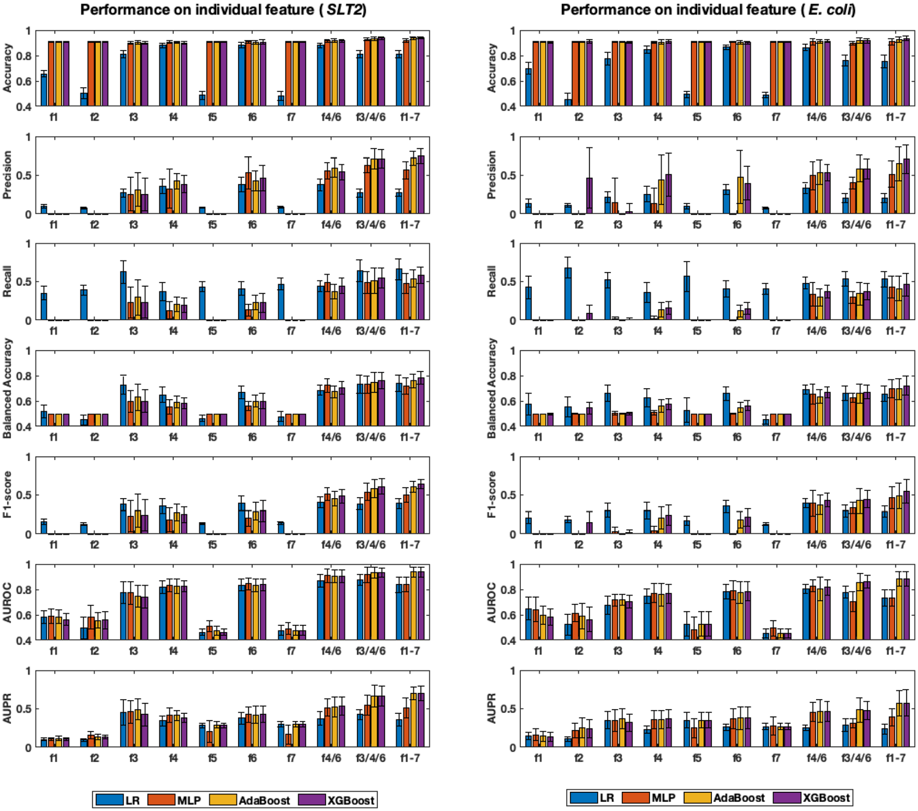
Classification performance on individual features within G1 feature group. Seven individual features are denoted by f1, f2, etc. and combined features are denoted by f4/6, f3/4/6, and f1-7, respectively. Standard deviation is represented by error bars and the range of y-axis is adjusted to emphasize changes in values.

We further investigated feature importance by combining multiple features as follows: f4 and f6 (denoted as f4/6); f3, f4, and f6 (denoted as f3/4/6); and all seven features, which is G1 (also denoted as f1–7) in Figure 3. The three attributes, f3, f4, and f6, are the high important attributes by Eppenhof and Peña-Castillo.³⁰ The intuition behind this combination is that combining important attributes results in a more important feature set. More careful visual inspection was needed to observe the improvement of accuracy with the extension as the change is relatively small, while the other five metrics clearly demonstrated improved performance along with the increased size of combined feature set, i.e. f4/6 ⩽ f3/4/6 ⩽ f1-7, where “⩽” indicates improved performance. Accordingly, G1 itself turned out to be the best combined feature group and it worked well with all seven metrics and four algorithms. Particularly, we found that AB and XGB performed well overall. Specifically, with G1 of STL2, AdaBoost and XGBoost achieved accuracy (0.937 ± 0.009, 0.942 ± 0.008), balanced accuracy (0.758 ± 0.053, 0.78 ± 0.049), precision (0.72 ± 0.088, 0.748 ± 0.09), recall (0.539 ± 0.113, 0.583 ± 0.107), F1-score (0.606 ± 0.068, 0.642 ± 0.056), AUROC (0.938 ± 0.038, 0.936 ± 0.041), and AUPR (0.698 ± 0.079, 0.701 ± 0.092), respectively. Also, with G1 of E. coli K12, AB and XGB achieved accuracy (0.925 ± 0.022, 0.933 ± 0.018), balanced accuracy (0.693 ± 0.08, 0.72 ± 0.076), precision (0.648 ± 0.217, 0.707 ± 0.185), recall (0.411 ± 0.154, 0.46 ± 0.15), F1-score (0.493 ± 0.165, 0.547 ± 0.148), AUROC (0.884 ± 0.058, 0.881 ± 0.055), and AUPR (0.569 ± 0.163, 0.575 ± 0.174), respectively.

The models evaluated with a single non-inclusive numerical feature and accuracy metric didn’t provide useful information regarding the importance of individual features. It rather gets stuck with the accuracy paradox as there exist imbalanced class distributions in both datasets. However, we observed that every feature captures a unique characteristic; thus, the combination of all seven features results in best classification performance. Our data confirm that features by Tang et al²⁹ and Eppenhof and Peña-Castillo³⁰ features work well for predicting sRNAs in our tested genomes.

Analysis of importance of individual feature groups (G1–G15)

We adopted the same idea of exploiting the importance of the individual features of G1 and recognized the importance of the individual feature groups. Like the individual features in the previous section, we measured classification performance on every individual feature group from G1 to G15 in terms of six learning algorithms with seven metrics. The overall performance was consistently similar, regardless of learning algorithms, evaluation metrics, and datasets with some variations; thus, we reported the performance only with the two best performing classifiers, AB and XGB in Figure 4.

Figure 4.

Classification performance on individual feature groups with AdaBoost and XGBoost. Left graphs represent classification performance for SLT2 and right ones are for the E. coli K12 dataset. Standard deviation is represented by error bars and y-axis range is adjusted to emphasize changes in values.

Tang et al²⁹ analyzed contributions of individual feature-based predictors as weights to their ensemble model, called WAEM, and concluded that all individual feature-based predictors were useful for improving the sRNA predicting performance. Specifically, they recognized the importance of individual features as follows: high (G4 (F4), G6 (F5), G10 (F12), G11 (F13), and G13 (F14)); and low (G2 (F1), G3 (F2), G7 (F9), G8 (F10), G12 (F14), and G15 (F17)). See the detailed discussion on the optimal weights for their WAEM models in Figure 4 by Tang et al.²⁹ Referring the seven subplots in Figure 4, we recognized the importance of individual feature groups as follows: high (G10 and G11), medium high (G4, G5, G6, and G13), medium low (G8 and G12), and low (G2, G7, and G15), which is consistent with what Tang et al²⁹ observed in their study. Notice that Tang et al²⁹ obtained the feature group importance as the contribution (or weight) to their specific ensemble model, while we recognized the feature group importance by directly measuring the classification performance in terms of evaluation metrics, when a single feature group was used as an input for learning algorithms, as we did for the assessment of the feature importance.

Still, G1 yielded stable results over all the algorithms as well as it performed better than the remaining 14 feature groups (G2–G15). Among the remaining 14 feature groups, G11 results in the second-best performance and G7 performed the worst. We observed during the experimental study that the low performing single feature groups, particularly G2 and G7, incorrectly classified all test data into the negative class (i.e. one class assignment). Tang et al²⁹ hinted that no feature groups extremely poorly performed and different features could bring different information. Thus, we tested the performance with the two combined groups: G2–14 and G1–15. As displayed in Figure 4, G2–14 improved performance better than the other 14 feature groups (i.e. G2 to G15) and G1–15 improved it further, close to or slightly better than G1’s performance. Therefore, we conclude that the most consistent and optimal performance for each model comes from the use of all combined feature groups (G1–15) rather than a single feature group.

Assessment of classification performance on combined feature groups

We considered 15 sequence characterizations (G1–G15) of each single sRNA sequence to numerical features. We employed six classification algorithms and seven performance assessment metrics. Then, we separately explored how classification performance changed with individual features, with individual feature groups, and with combined feature groups. Through stratified 10-fold CV, we recognized the three best forming groups of features, G1(7), G2–15(2222), and G1–15(2229) and illustrated their performance in Figures 3 and 4.

G2–15(2222) feature group is a combination of 14 feature groups, which was a subset of the original feature groups by Tang et al.²⁹ It includes 2222 numerical features, which are independent from the seven features of G1(7) feature group. The 10-fold CV performance for G2–15(2222) feature group is better than each of the 14 individual feature groups as shown in Figure 4; however, it turned out that its performance is worse than the performance of G1(7).

G1–15(2229) is a combination of G1(7) and G2–15(2222), by which it was intended to combine different information in the two sets of feature groups. It results in a total of 2229 numerical features. We found that G1–15 performed consistently better than G2–15 feature group and G1(7) feature group as shown Figures 4 and 5. Particularly, G1–15(2229) achieves best performance with AdaBoost and XGBoost algorithms, beating the two other tree-based ensemble methods, GB and RF. Furthermore, it highlights best performance when it is combined with AUROC and AUPR with stratified k-fold CV.

Figure 5.

Classification performance on combined feature groups. Left graphs represent classification performance for SLT2 and right ones are for E. coli K12 dataset. Standard deviation is represented by error bars and y-axis range is adjusted to emphasize changes in values.

After inspecting the confusion matrix for each of the 10-fold CV folds, we found that both GB and RF assigned every input to the negative label instead of learning to differentiate the two class labels. This one class assignment resulted in a low AUROC for both models. Meanwhile, both AdaBoost and XGBoost demonstrated similar performance, maintaining the high performance with the larger feature set. Specifically, this result hinted that the combined feature group, G1–15, might be a good feature set that matched well with specific learning models and evaluation metrics, resulting in the robust classification performance in learning the imbalanced class distributions.

As recommended in the literature, the four metrics, including balanced accuracy, F1-score, AUROC, and AUPR, worked consistently with imbalanced class distributions. Particularly, AdaBoost and XGBoost with the largest feature set (G1–15) were consistently learning and accurately classifying the sequences. Another result worth noting is that the model comparisons consistently hold for the two datasets that were tested.

Performance with varying positive-to-negative instance ratios

Another variable factor that may affect the performance of machine learning models is the positive-to-negative (or negative-to-positive) instance ratio. We assessed the performance of all six learning algorithms using the positive-to-negative instance ratios from one balanced ratio (1-to-1) to nine imbalanced ones (from 1-to-2 to 1-to-10). For example, we used all the known sRNA sequences as positive ones and adjusted the number of negative sequences so that the correct number of negative sequences for the specified ratio can be fed to the learning algorithm.

As before, the overall performance was consistently similar with a little variation, regardless of algorithms, metrics, and feature groups. Specifically, we observed three patterns of classification performance change over varying positive-to-negative data ratios of the largest feature group (i.e. G1-15 with 2,229 features) as shown in Figure 6: increasing, stable, and decreasing upon increasing negative-to-positive instance ratios. Similar patterns were also observed in other individual feature groups (not reported). Specifically, as in the previous study by Tang et al,²⁹ we found that accuracy increases as the number of negative instances increases, which means that the highest accuracy value was obtained at the positive-to-negative instance ratio of 1-to-10. In this case, it is highly probable that the learning algorithm experiences the accuracy paradox condition, simply by assigning class labels to the major class. Therefore, it is known that accuracy is not a reasonable metric for imbalanced data distributions. Only AUROC performance maintains the stable (or horizontal) pattern without much up and down fluctuations over varying imbalance ratios. Assume the case that the learning algorithm experiences the accuracy paradox because of the imbalanced class distributions. Therefore, if AUROC remaining the stable pattern as shown in Figure 6, then AUROC might not be appropriate for the case. We found that the remaining performance plots with precision, recall, balanced accuracy, F1-score, and AUPR show a decreasing trend along with an increase of the positive-to-negative imbalance instance ratios.

Figure 6.

Classification performance change over varying positive-to-negative data ratios of G1-15 feature group. Left graphs represent classification performance for SLT2 and right ones are for E. coli K12 dataset. Standard deviation is represented by error bars and y-axis range is adjusted to emphasize changes in values.

The increasing or decreasing trends over the increasing negative-to-positive instance ratios might be applicable to recognize the balancing factor (i.e. the ratio between positive and negative instances) and/or the class labels of a set of instances as the expected trends can be estimated with adding and removing known instances. Accordingly, it can be a potential future work as it might be also adaptable to an online learning scenario with streamlining data.

Conclusion

The mean lengths of sRNAs in SLT2 and E. coli K12 are greater than the corresponding median as well as the grouped length distributions are skewed, which partially supports the criteria that obey Benford’s law. However, the expanded conformity tests (MAD, K-S test, and Chi-square test) do support for the 99.9% confidence interval, while it does not fully support for the 95% confidence interval. The deviations from Benford’s law might be attributed to the small subset (or sample) problem, lacking statistical power and representativeness, or a latent bias of different sRNA dynamics of functional domains toward interaction with their target genes.

Different from Eppenhof and Peña-Castillo³⁰ and Tang et al,²⁹ we identified importance individual features (or feature groups) by directly measuring the performance of the metrics when a single attribute (or a single feature group) was used as an input for each learning algorithm, which is simpler and straight-forward. Three levels of feature importance in features in G1 feature group, previously identified in the literature, were recognized, including distance to the closest left ORF (f4), distance to the closest right ORF (f6), and distance to the closest Rho-independent terminator (f3)). Also, the levels of feature group importance, previously identified in the literature, were recognized, including 4-RCkmer (G10) and 5-RCkmer (G11) as best feature groups, while 1-mer (G2) and 1-RCkmer (G7) as worst performing feature groups.

Combining a few well-performing features worked better than a single feature and combining all seven features (i.e. G1(7)) performed better than combining a few features as well as G2–15(2222) feature group. The best performing feature set is G1–15(2229), which consists of G1(7) and G2–15(2222). We validated that no single feature group performed extremely poorly, and different features could bring different information. GB and RF tended to result in one-class assignment as the feature set size increased. AdaBoost and XGBoost with G1–15 feature group consistently generated high AUROC and AUPR values, indicating that both models similarly learned well for all experimental settings. AdaBoost and XGBoost with G1–15 feature group performed better with increased features. Therefore, it is worth extending this study to validate the performance of the two ensemble learning algorithms with sRNAs in more genomes available in biological databases.

Supplemental Material

sj-xlsx-1-bbi-10.1177_11779322221118335 – Supplemental material for Prediction of Bacterial sRNAs Using Sequence-Derived Features and Machine Learning

Supplemental material, sj-xlsx-1-bbi-10.1177_11779322221118335 for Prediction of Bacterial sRNAs Using Sequence-Derived Features and Machine Learning by Tony Jha, Jovinna Mendel, Hyuk Cho and Madhusudan Choudhary in Bioinformatics and Biology Insights

Footnotes

Funding:

The author(s) disclosed receipt of the following financial support for the research, authorship, and/or publication of this article: This work was supported by the National Science Foundation (USA), Award #2050232 to Madhusudan Choudhary (PI) and Hyuk Cho (Co-PI). Tony Jha, an undergraduate at University of California at Berkeley received a stipend for the 2021 summer research REU program.

Declaration of Conflicting Interests:

The author(s) declared no potential conflicts of interest with respect to the research, authorship, and/or publication of this article.

Author Contributions

This work is a product of the intellectual effort of the whole team and that all members have contributed in various degrees to the analytical methods used, the research concept, the experiment design, and the manuscript preparation.

Supplemental Material

Supplemental material for this article is available online.

References

Waters

Storz

. Regulatory RNAs in bacteria. Cell. 2009;136:615-628. doi:10.1016/j.cell.2009.01.043.

Ying

Chen

. Predicting sRNAs and Their Targets in Bacteria. Genomics Proteomics Bioinformatics. 2012;10:276-284. doi:10.1016/j.gpb.2012.09.004.

Fuli

Wenlong

Xiao

, et al. A genome-wide prediction and identification of intergenic small RNAs by comparative analysis in Mesorhizobium huakuii 7653R. Front Microbiol. 2017;8:1730-1730. doi:10.3389/fmicb.2017.01730.

Ellis

Trussler

Haniford

. A cis-encoded sRNA, Hfq and mRNA secondary structure act independently to suppress IS200 transposition. Nucleic Acids Res. 2015;43:6511-6527. doi:10.1093/nar/gkv584.

Bloch

Węgrzyn

Nejman-Faleńczyk

. Small and smaller-sRNAs and MicroRNAs in the regulation of toxin gene expression in prokaryotic cells: a mini-review. Toxins (Basel). 2017;9:181. doi:10.3390/toxins9060181.

Gottesman

. Micros for microbes: non-coding regulatory RNAs in bacteria. Trends Genet. 2005;21:399-404. doi:10.1016/j.tig.2005.05.008.

Storz

Vogel

Wassarman

. Regulation by small RNAs in bacteria: expanding frontiers. Mol Cell. 2011;43:880-891. doi:10.1016/j.molcel.2011.08.022.

Bos

Duverger

Thouvenot

, et al. The sRNA RyhB regulates the synthesis of the Escherichia coli methionine sulfoxide reductase MsrB but Not MsrA. PLoS ONE. 2013;8:e63647. doi:10.1371/journal.pone.0063647.

Baker

Eöry

Yakhnin

Mercante

Romeo

Babitzke

. CsrA inhibits translation initiation of Escherichia coli hfq by binding to a single site overlapping the Shine-Dalgarno sequence. J Bacteriol. 2007;189:5472-5481. doi:10.1128/jb.00529-07.

10.

Azam

Vanderpool

. Translation inhibition from a distance: The small RNA SgrS silences a ribosomal protein S1-dependent enhancer. Mol Microbiol. 2020;114:391-408. doi:10.1111/mmi.14514.

11.

Soper

Mandin

Majdalani

Gottesman

Woodson

. Positive regulation by small RNAs and the role of Hfq. Proc Natl Acad Sci USA. 2010;107:9602-9607. doi:10.1073/pnas.1004435107.

12.

Chen

Morita

Gottesman

. Regulation of transcription termination of small RNAs and by small RNAs: molecular mechanisms and biological functions. Front Cell Infect Microbiol. 2019;9:201. doi:10.3389/fcimb.2019.00201.

13.

Holmqvist

Wagner

EGH

. Impact of bacterial sRNAs in stress responses. Biochem Soc Trans. 2017;45:1203-1212. doi:10.1042/bst20160363.

14.

Mohd-Padil

Damiri

Sulaiman

Chai

S-F

Nathan

Firdaus-Raih

. Identification of sRNA mediated responses to nutrient depletion in Burkholderia pseudomallei. Sci Rep. 2017;7:17173. doi:10.1038/s41598-017-17356-4.

15.

Thomason

Fontaine

De Lay

Storz

. A small RNA that regulates motility and biofilm formation in response to changes in nutrient availability in Escherichia coli. Mol Microbiol. 2012;84:17-35. doi:10.1111/j.1365-2958.2012.07965.x.

16.

Coornaert

Mandin

Springer

Gottesman

Guillier

. MicA sRNA links the PhoP regulon to cell envelope stress. Mol Microbiol. 2010;76:467-479. doi:10.1111/j.1365-2958.2010.07115.x.

17.

Guo

Updegrove

Gogol

Shabalina

Gross

Storz

. MicL, a new σE-dependent sRNA, combats envelope stress by repressing synthesis of Lpp, the major outer membrane lipoprotein. Genes Dev. 2014;28:1620-1634. doi:10.1101/gad.243485.114.

18.

Papenfort

Pfeiffer

Mika

Lucchini

Hinton

Vogel

. SigmaE-dependent small RNAs of Salmonella respond to membrane stress by accelerating global omp mRNA decay. Mol Microbiol. 2006;62:1674-1688. doi:10.1111/j.1365-2958.2006.05524.x.

19.

Barshishat

Elgrably-Weiss

Edelstein

, et al. OxyS small RNA induces cell cycle arrest to allow DNA damage repair. Embo J. 2018;37:413-426. doi:10.15252/embj.201797651.

20.

Gao

Chen

Tian

, et al. The novel ncRNA OsiR positively regulates expression of katE2 and is required for oxidative stress tolerance in Deinococcus radiodurans. Int J Mol Sci. 2020;21:3200. doi:10.3390/ijms21093200.

21.

Fröhlich

Gottesman

. Small regulatory RNAs in the enterobacterial response to envelope damage and oxidative stress [published online ahead of print July 6, 2018]. Microbiol Spectr. doi:10.1128/microbiolspec.RWR-0022-2018.

22.

Lalaouna

Baude

, et al. RsaC sRNA modulates the oxidative stress response of Staphylococcus aureus during manganese starvation. Nucleic Acids Res. 2019;47:9871-9887. doi:10.1093/nar/gkz728.

23.

Chakravarty

Massé

. RNA-dependent regulation of virulence in pathogenic bacteria. Front Cell Infect Microbiol. 2019;9:337-337. doi:10.3389/fcimb.2019.00337.

24.

Bobrovskyy

Vanderpool

. Regulation of bacterial metabolism by small RNAs using diverse mechanisms. Annu Rev Genet. 2013;47:209-232. doi:10.1146/annurev-genet-111212-133445.

25.

Jørgensen

Pettersen

Kallipolitis

. sRNA-mediated control in bacteria: An increasing diversity of regulatory mechanisms. Biochim Biophys Acta Gene Regul Mech. 2020;1863:194504. doi:10.1016/j.bbagrm.2020.194504.

26.

Altuvia

. Identification of bacterial small non-coding RNAs: experimental approaches. Curr Opin Microbiol. 2007;10:257-261. doi:10.1016/j.mib.2007.05.003.

27.

Georg

Lalaouna

Hou

, et al. The power of cooperation: experimental and computational approaches in the functional characterization of bacterial sRNAs. Mol Microbiol. 2020;113:603-612. doi:10.1111/mmi.14420.

28.

Grüll

Peña-Castillo

Mulligan

Lang

. Genome-wide identification and characterization of small RNAs in Rhodobacter capsulatus and identification of small RNAs affected by loss of the response regulator CtrA. RNA Biol. 2017;14:914-925.

29.

Tang

Shi

Yue

Zhang

. Sequence-based bacterial small RNAs prediction using ensemble learning strategies. BMC Bioinformatics. 2018;19:503. doi:10.1186/s12859-018-2535-1.

30.

Eppenhof

EJJ

Peña-Castillo

. Prioritizing bona fide bacterial small RNAs with machine learning classifiers. PeerJ. 2019;7:e6304. doi:10.7717/peerj.6304.

31.

Ostir

Uchida

. Logistic regression: a nontechnical review. Am J Phys Med Rehabil. 2000;79:565-572. doi:10.1097/00002060-200011000-00017.

32.

Castro

Oblitas

Santa-Cruz

Avila-George

. Multilayer perceptron architecture optimization using parallel computing techniques. PLoS ONE. 2017;12:e0189369. doi:10.1371/journal.pone.0189369.

33.

Freund

Schapire

. Experiments with a new boosting algorithm. Paper presented at: Proceedings of the Thirteenth International Conference on International Conference on Machine Learning; July 3-6, 1996; Bari, Italy.

34.

Natekin

Knoll

. Gradient boosting machines, a tutorial. Front Neurorobot. 2013;7:21-21. doi:10.3389/fnbot.2013.00021.

35.

Breiman

. Random forests. Machine Learn. 2001;45:5-32. doi:10.1023/A:1010933404324.

36.

Chen

Guestrin

. XGBoost: a scalable tree boosting system. Paper presented at: Proceedings of the 22nd ACM SIGKDD International Conference on Knowledge Discovery and Data Mining; August 13-17, 2016:785-794; San Francisco, CA.

37.

Liu

Fang

Wang

Chou

. repDNA: a Python package to generate various modes of feature vectors for DNA sequences by incorporating user-defined physicochemical properties and sequence-order effects. Bioinformatics. 2015;31:1307-1309. doi:10.1093/bioinformatics/btu820.

38.

Krawczyk

. Learning from imbalanced data: open challenges and future directions. Progress in Artificial Intelligence. 2016;5:221-232. doi:10.1007/s13748-016-0094-0.

39.

Haibo

Yunqian

. Imbalanced datasets: from sampling to classifiers. In: He

, eds. Imbalanced Learning: Foundations, Algorithms, and Applications. New York, NY: IEEE; 2013:43-59.

40.

Valverde-Albacete

Peláez-Moreno

. 100% Classification Accuracy Considered Harmful: The Normalized Information Transfer Factor Explains the Accuracy Paradox. PLoS ONE. 2014;9:e84217. doi:10.1371/journal.pone.0084217.

41.

Xingquan

Ian

, eds. Knowledge Discovery and Data Mining: Challenges and Realities. Hershey, PA: IGI Global; 2007.

42.

Ciza

Balakrishnan

. Improvement in minority attack detection with skewness in network traffic. https://ui.adsabs.harvard.edu/abs/2008SPIE.6973E..0NT/abstract. Published 2008.

43.

Fernandes

Irigoien

Goikoetxea

, et al. Fish recruitment prediction, using robust supervised classification methods. Ecol Model. 2010;221:338-352. doi:10.1016/j.ecolmodel.2009.09.020.

44.

Pedregosa

Varoquaux

Gramfort

, et al. Scikit-learn: machine learning in Python. J Mach Learn Res. 2011;12:2825-2830.

45.

Brodersen

Ong

Stephan

Buhmann

. The balanced accuracy and its posterior distribution. Paper presented at: 2010 20th International Conference on Pattern Recognition; August 23-26, 2010:3121-3124; Istanbul, Turkey.

46.

Kelleher

Namee

D’Arcy

. Fundamentals of Machine Learning for Predictive Data Analytics: Algorithms, Worked Examples, and Case Studies. Cambridge, MA: The MIT Press; 2015.

47.

van Rijsbergen

. Information retrieval: new directions: old solutions. Paper presented at: Proceedings of the 6th Annual International ACM SIGIR Conference on Research and Development in Information Retrieval; June 6-8, 1983; Bethesda, MD. doi:10.1145/511793.511831.

48.

Fawcett

. An introduction to ROC analysis. Pattern Recogn Lett. 2006;27:861-874. doi:10.1016/j.patrec.2005.10.010.

49.

Davis

Goadrich

. The relationship between Precision-Recall and ROC curves. Paper presented at: Proceedings of the 23rd International Conference on Machine Learning; June 25, 2006; Pittsburgh, PA. doi:10.1145/1143844.1143874.

50.

Saito

Rehmsmeier

. The precision-recall plot is more informative than the ROC plot when evaluating binary classifiers on imbalanced datasets. PLoS ONE. 2015;10:e0118432. doi:10.1371/journal.pone.0118432.

51.

Lever

Krzywinski

Altman

. Classification evaluation. Nat Methods. 2016;13:603-604. doi:10.1038/nmeth.3945.

52.

Jung

. A K-fold averaging cross-validation procedure. J Nonparametr Stat. 2015;27:167-179. doi:10.1080/10485252.2015.1010532.

53.

Newcomb

. Note on the frequency of use of the different digits in natural numbers. Am J Math. 1881;4:39-40.

54.

Benford

. The law of anomalous numbers. Proc Am Philos Soc. 1938;78:551-572.

55.

Nigrini

Wells

. Benford’s Law: Applications for Forensic Accounting, Auditing, and Fraud Detection. New York, NY: Wiley; 2012.

56.

Pietronero

Tosatti

Vespignani

. Explaining the uneven distribution of numbers in nature: the laws of Benford and Zipf. Physica A. 2001;293:297-304. doi:10.1016/S0378-4371(00)00633-6.

57.

Friar

Goldman

Pérez-Mercader

. Genome sizes and the Benford distribution. PLoS ONE. 2012;7:e36624. doi:10.1371/journal.pone.0036624.

Supplementary Material

Please find the following supplemental material available below.

For Open Access articles published under a Creative Commons License, all supplemental material carries the same license as the article it is associated with.

For non-Open Access articles published, all supplemental material carries a non-exclusive license, and permission requests for re-use of supplemental material or any part of supplemental material shall be sent directly to the copyright owner as specified in the copyright notice associated with the article.

0.00 MB

0.06 MB