Sage Journals: Discover world-class research

Abstract

The problem of selecting important variables for predictive modeling of a specific outcome of interest using questionnaire data has rarely been addressed in clinical settings. In this study, we implemented a genetic algorithm (GA) technique to select optimal variables from questionnaire data for predicting a five-year mortality. We examined 123 questions (variables) answered by 5,444 individuals in the National Health and Nutrition Examination Survey. The GA iterations selected the top 24 variables, including questions related to stroke, emphysema, and general health problems requiring the use of special equipment, for use in predictive modeling by various parametric and nonparametric machine learning techniques. Using these top 24 variables, gradient boosting yielded the nominally highest performance (area under curve [AUC] = 0.7654), although there were other techniques with lower but not significantly different AUC. This study shows how GA in conjunction with various machine learning techniques could be used to examine questionnaire data to predict a binary outcome.

Keywords

genetic algorithm machine learning NHANES questionnaire

Introduction

High-dimensional datasets provide many mathematical and statistical challenges, as well as some opportunities, and will likely lead to novel theoretical developments. A major challenge of dealing with high-dimensional datasets is that, in many cases, not all the measured variables are considered important for understanding the underlying phenomena of interest.¹ While certain computationally expensive techniques² can construct predictive models with considerable accuracy from high-dimensional data, reduction of these data prior to modeling is a separate problem that has received recent attention. Genetic algorithms (GAs), in particular, provide an attractive approach to reduce such a dataset.³ The GA method, compared to other popular methods, offers a wider solution space; handles noisy functions well; handles large, poorly understood search spaces easily; and can be easily modified for different problems.⁴

Over the years, GA methodology has evolved, as has the range of its applications. GAs have been employed in searching for the best subset of single nucleotide polymorphisms (SNPs) associated with a phenotype,^5–10 searching for the shortest route and multiple semishortest routes in one search,¹¹ and prediction of small molecule binding modes to macromolecules.¹²

Surveys and questionnaires are widely used in various areas of research, especially in health-related fields, as they provide a relatively efficient method of sampling many individuals in an inexpensive and less obtrusive manner.^13,14 Questionnaires have been used to study musculoskeletal, psychological, cardiovascular, and other disorders,^15–21 and as the popularity of questionnaires has grown, so has the potential for new understanding via advanced statistical techniques such as GA. Although GA has been successfully applied to questionnaire variable selection in the context of family medicine, stressful life events,²² and sleep apnea diagnosis,²³ its application to the selection of questionnaire data for predictive modeling of disease outcome is relatively novel. Outside biomedical research, Madden utilized GAs in the analysis of questionnaire data to ascertain students’ attitudes toward their schoolwork, showing that GAs may be used to generate logical rules, which predict one variable in relation to others.²⁴ Additionally, Yukselturk et al applied GA in predicting student dropout utilizing only 10 variables.²⁵

GAs use a heuristic search and optimization method inspired by natural evolution and have been successfully applied to a wide range of complex real-world problems. Beginning with a randomly generated population of chromosomes (potential solutions), the algorithm carries out a process of fitness-based selection in which the parent chromosomes are recombined to generate a successor population. The process is iterated, evolving a sequence of successive generations, until the average fitness of chromosomes increases to reach a stopping criterion. Thus, GAs evolve a best solution to a given problem according to the specified fitness function.²⁶ The detailed theories behind GA are beyond the scope of this article but are discussed in other publications.^27–29

In our study, GA was used to select questions from the 1999 to 2000 National Health and Nutrition Examination Survey (NHANES) most predictive of five-year mortality as indicated in a follow-up survey. Specifically, GA selected the top 24 questions from an initial 123 variables. Utilization of these 24 variables and selected variable subsets for predictive modeling, using five-year mortality as the outcome of interest, was carried out using a variety of machine learning methods, including gradient boosting, artificial neural network (ANN), elastic net, support vector machine (SVM), ridge regression (RR), logistic regression, random forest, least absolute shrinkage and selection operator (LASSO), partial least squares-discriminant analysis (PLS-DA), and classification trees (implemented in the R package RPART [recursive partitioning and regression trees]). All of these techniques yielded optimum results when all 24 variables were included in the analysis, with gradient boosting demonstrating the best nominal performance.

Methods

Variable quality control and imputation

Participants with linked mortality data from the NHANES (1999-2000) were included in the study (Table 1). The NHANES is designed to monitor the health and nutritional status of the American civilian population using annual interviews and medical examinations. Mortality data were accessed from the National Death Index (NDI) with an end point of December 2006.³⁰ The 1999-2000 NHANES questionnaire data initially included a heterogeneous cohort of 9,965 individuals who answered 2,058 questions (variables), 5,444 of whom had available five-year mortality data and were included in the current study (412 cases/5,032 controls) (Table 1). Variables with > 30% missing information or zero variance were removed from the analysis, as were groups of highly collinear variables. All data were transformed to an integer scale with uniform directionality, with higher numerical responses indicating poorer health status. For variables where directionality was not explicit, the order was inferred from factors known to contribute to mortality. Variables that could not be transformed in this manner were removed, generating 123 variables to be used in our final analysis. Missing information for the remaining variables was imputed using Amelia II as required for implementation of GALGO GA software in R.^31,32 Amelia II imputes missing values using the expectation-maximization (EM) with bootstrapping algorithm. The algorithm utilizes the familiar EM algorithm on multiple bootstrapped samples of the original incomplete data to draw values of the complete-data parameters.³¹ Historically, the rule of thumb for multiple imputations is to use M = 5.³³ We took the average of five imputation results and rounded the numerical responses to the nearest whole numbers according to the initial responses given. In order to circumvent the further effects of variable missingness or strong correlations among our variables, as well as the effects of the number of observations (ie, 5,444 individuals) being higher than our number of parameters (ie, 2,058 questions), we implemented a ridge prior of at least 10% of our number of observations. This promotes numerical stability by shrinking the covariances among the variables toward zero without changing the means of variances.³¹

Table 1

Demographics of questionnaire respondents with available five-year mortality data.

Age	18-20	20-29	30-39	40-49	50-59	60-69	70-79	≥80
Individuals	568	871	824	763	585	817	594	422
Ethnicity	white^*	Black^*	Mexican American	Other Hispanic		Other Race/Multi-Racial
Individuals	2329	1035	1550	337		193

Note:

Non-Hispanic.

The data were then randomly divided into 70% training (3,810 individuals [288 cases/3,522 controls]) and 30% testing (1,634 individuals [124 cases/1,510 controls]) sets. GA was performed in the training set using the procedure described in the following section. The predictive ability of the variables selected by the GA was then determined in an independent testing set.

Genetic algorithm

GA is a feature selection method that identifies variables that are most likely predictors of a given binary outcome. The procedure starts by generating a random population of variable clusters. These clusters, or chromosomes, are then assessed for their ability to accurately predict the binary outcome using a nearest centroid fitness function, which has been found to outperform other multivariate selection functions, including random forests and SVMs, when paired with GA. ³² In general, the initial variable cluster is mutated to form a new cluster of variables with higher classification accuracy, and the process is repeated until a desired level of accuracy is achieved.^28,32 GA is advantageous in that during the exploration of the space of possible solutions, it does not evaluate solutions one by one but evaluates a set of solutions simultaneously. Moreover, it is less prone to entrapment within local minima and does not require assumptions about the interactions between features.^34,35 To overcome the inherent problems of randomized algorithms, however, it is occasionally proposed that GA be run multiple times on a given optimization problem to provide the best solution.³⁶ Thus, we implemented 10 GA iterations to select NHANES questionnaire variables predictive of five-year mortality and considered the average output of GA. Further information about GA can be found in several references.^4,27–29

Machine learning techniques

The optimally selected variables from the GA were then used to build predictive models using various machine learning techniques, including gradient boosting, ANN, elastic net, SVM, RR, logistic regression, random forest, LASSO, PLS-DA, and Classification Trees, with optimized parameters (Table 2). These algorithms were then compared to determine the technique and set of variables demonstrating the most accurate prediction. All machine learning technique calculations were performed using various R packages under R version 3.1.2.^37–45 While the intent of this article is to compare the predictive performances of various machine learning algorithms, we also provide some background about these methods to assist the readers.

Table 2

Fine-tuning parameters for ANN, gradient boosting, SVM, PLS-DA, elastic net, and random forests to achieve the highest AUC values in the test set (f = frequency).

TECHNIQUE		TOP 24 QUESTIONS	TOP 13 QUESTIONS (f > 0.2)	TOP 9 QUESTIONS (f < 0.3)	TOP 5 QUESTIONS (f > 0.4)	TOP 3 QUESTIONS (f= 1.0)
ANN	Hidden layers	3	30	50	3	3
	Decay parameter	0.04	0.04	0.04	0.001	0.04
Gradient boosting	Number of trees	5000	10000	5000	1000	10000
	Interaction depth	4	1	1	3	2
SVM	Gamma	10^-6	10^-5	10	10^-4	2
	Epsilon	1	1	1	1	0.01
PLS-DA	Factors (14 questions only)	8	–	–	–	–
Elastic net	Elastic Net mixing parameter (alpha)	0.01	0.1	0.1	0.2	0.1
Random forest	Node size	50	50	50	10	10
	Number of trees	10	10	10	10	10

Gradient boosting

This is a general method for improving the accuracy of any given learning technique. In this approach, the goal is to approximate the functional relationship between independent variables and the outcome variable by minimizing some prespecified loss function. This process involves the combination and weighting of many relatively weak or inaccurate rules (usually decision tree models) to produce an ensemble predictor with higher predictive accuracy.⁴⁶

Artificial neural network

Artificial neural networks are a family of machine learning techniques that are modeled after biological networks of neurons. This technique attempts to infer the relationship between a set of inputs and an outcome of interest by using learning algorithms to assign numeric weight to each input measurement. The sum of the weighted inputs is used for outcome prediction.⁴⁷

Elastic net

This technique combines the LASSO and ridge penalties, yielding an intermediate penalty with typically fewer regression coefficients approximating to zero than LASSO. Like LASSO, it is particularly useful for variable selection in high-dimensional settings, producing sparse models that preserve predictive power and encourage grouping of correlated predictors.⁴⁸

support vector machine

This algorithm involves projection of the data points in a training set with n input variables into n-dimensional space and the construction of an (n — 1)-dimensional surface (called a hyperplane) that maximizes the distance between cases and controls (or any binary categorization). New samples are then mapped into the same space, and the binary outcome is predicted based upon which side of the hyperplane each sample falls on.⁴⁹

Ridge regression

This method is an extension of classical regression that involves imposing a constraint on the sum of the squares of the regression coefficients such that they do not exceed a chosen tuning parameter. The effect of this is to shrink the regression coefficient estimates to small, nonzero values. This approach exploits the bias-variance tradeoff, reducing variance of the coefficient estimates by increasing their bias. This shrinkage of coefficients prevents overfitting by compensating for the variance inflation that occurs due to multicollinearity. This technique is particularly powerful for high-dimensional problems.⁵⁰

Logistic regression

This simple method is a special case of generalized linear models that evaluates the dependence of a binary variable on one or more independent variables using maximum likelihood techniques. It is intrinsically simple and valuable in solving binary classification problems.⁵¹

Random forest

This algorithm involves constructing a collection of decision trees using rule-based classification or regression methods. Each tree is constructed from a bootstrap sample extracted from the training set and is developed independently of others. A large number of trees constructed this way are used to form an ensemble (known as a forest) that collectively votes to optimally classify input vectors.^2,52

LASSO regression

Like RR, this method is an extension of classical regression but uses a different penalty. This penalty involves constraining the sum of the absolute values of the regression coefficients such that they do not exceed a chosen tuning parameter. Unlike RR, some coefficients may shrink to zero, making LASSO especially useful for variable selection problems. The result is a set of solutions that are shrunken versions of the typical least-squares estimates as in the case of linear regression, compensating for overfitting that may occur in the presence of multicollinearity, or in high-dimensional settings.⁵³

Partial least squares-discriminant analysis

In PLS-DA, the goal is to reduce the dimensionality of data with a large number of input variables, while simultaneously accounting for membership in classes representing categories of some discrete (eg, binary) outcome. Dimension-reduction is carried out by the construction of new variables (referred to as latent variables) using linear combinations of the input variables. The linear combinations are generated in such a way as to maximize correlation of the latent variables with the categorical outcome. This resulting model can then be used to carry out predictions for new samples.⁵⁴

classification trees

This is a powerful, intuitive non-parametric technique that involves binary recursive splitting of a training set into increasingly homogeneous subsets using the input variables. This produces a tree-like construct (known as a decision tree) that, after being optimized, can be used to categorize new samples.⁵⁵

Assessing model performance

Given a binary classification that can be positive or negative, the area under the receiver operating characteristic curve (area under curve [AUC]) measures the probability that a prediction method will rank a randomly chosen positive sample over a randomly chosen negative sample. Thus, AUC = 1 represents a perfect model and AUC = 0.5 represents a model that yields no advantage over random guessing. AUC is useful in that it is calculated from the direct value output of a prediction method across all thresholds rather than the binary output dependent upon threshold placement. Additionally, it does not vary with the distribution of class labels in the sample set.⁵⁶ We implemented the pROC package to calculate the AUCs.⁵⁷

Results and Discussion

From an initial 2,058 variables (questions), 123 remained after excluding variables with > 30% missing information, zero variance, or collinearity (Table 3). Data from this initial preprocessing were then subjected to imputation using Amelia II as required for the GA analysis using GALGO.^31,32

Table 3

Breakdown of variables used in the analyses.

VARIABLE	NUMBER
Initial	2058
> 30% missing	1929
Zero variance	1
Perfectly collinear	5
Final	123

GA was performed using the 123 variables (ie, questions, Supplementary Table 1) and the training set consisting of 3,810 individuals. The default configuration shows three plots summarizing the characteristics of the population of selected chromosomes (Supplementary Fig. 1) or, within the context of our study, variable clusters. The topmost plot shows the number of times each gene (ie, question/variable) is present in a stored chromosome. By default, the top 50 genes are colored, whereas the top 7 are labeled (variables 24, 27, 55, 59, 60, 90, and 118). From the plot (Supplementary Fig. 1, top), it is apparent that variable 60 was included most frequently in the stored chromosomes, followed by variables 90 and 59. Also frequently included were variables 24, 27, 55, and 118. Once the top-ranked genes are stabilized, a second plot shows the stability of the rank of the top 50 genes (Supplementary Fig. 1, middle), aiding in the decision of whether or not to continue the process further. Unstable genes that demonstrate inconsistent rank or importance are indicated by numerous colors besides black and gray. Commonly, the top 7 black genes are stabilized quickly, in 100-300 solutions, whereas low-ranked gray genes would require thousands of solutions to be stabilized. Again, the top 7 aforementioned variables were the most highly ranked in this GA run, suggesting that they are the most important questions for predicting mortality. Finally, the bottom plot displays the distribution of the number of generations needed by the GA process to produce a solution (Supplementary Fig. 1), indicating how difficult the search problem is for the configuration of GA.

Before further analysis and refinement were performed, we first determined whether we were getting acceptable solutions. The success of the configured GA search can be determined by looking at the evolution of the fitness value across generations. On average, GA reached a solution in generation 4, which indicates an excellent result (Supplementary Fig. 2). The blue and cyan lines show the average fitness for all chromosomes and for those that have not reached a goal, respectively. These lines delimit an empirical confidence interval for the fitness across generations. The characteristic plateau effect is useful to decide whether or not the search is working effectively to reach our goal, which is marked with a dotted line. In general, our result indicates that we have achieved a stable solution within early generations.

Stochastic searches such as the GA are very efficient methods to identify solutions to an optimization (ie, classification) problem. However, they only explore a small portion of the total model space. The starting point of any GA search is a random population. This implies that different searches are likely to provide different solutions. As such, in order to extensively explore the entire space of models, it is critical to collect a large number of chromosomes. GALGO offers a diagnostic tool to determine when the GA searches reach some degree of convergence. This analysis is simply based on the frequency with which each gene (ie, question) appears in the chromosome population. As chromosomes (ie, variable clusters) are selected, the frequency of each gene in the population changes until no new solutions are found.³² Thus, we monitor the stability of gene ranks based on their frequency as a way to visualize model convergence (Supplementary Fig. 3). The most frequent 50 genes (ie, questions) are shown in eight different colors with about six or seven genes per color. 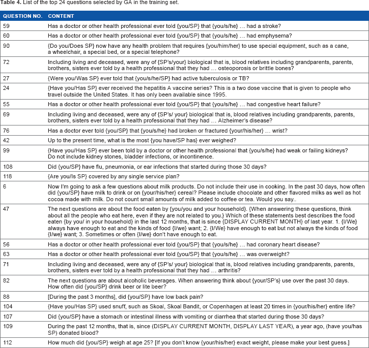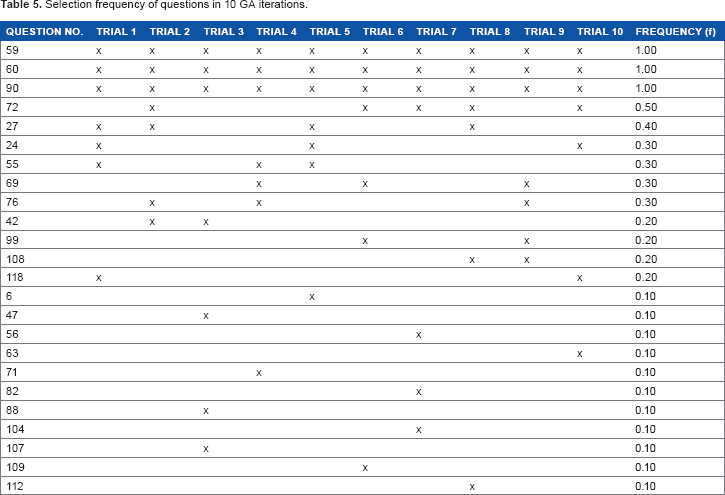The genes are ordered by rank along the horizontal axis, while the vertical axis indicates gene frequency (top portion of y-axis) and the color coded rank of each gene in previous evolutions (Supplementary Fig. 3). Changes in the ranks of the genes are coded by different colors (below the frequency). The top genes are stabilized in order with black genes first, then red, green, and so on, with the gray genes considered to be most unstable or of lowest priority (Supplementary Fig. 3).

Ten GA iterations using the training set data were performed using 123 questions, and each run generated seven questions, with some overlapping results. Multiple GA runs were used because multiple isolated iterations are more advantageous than a single GA run and reach the global solution using fewer function evaluations.⁵⁸ From the initial 123 variables, GA output the top 24 questions for predictive modeling strategies (Table 4). Investigation of the most stable results (black color coded genes, Supplementary Fig. 3) shows that questions 90, 59, and 60 are the most frequent variables appearing in each of the GA iterations (Table 5). Variable 90 is a question regarding health problems that require the participant to use special equipment, such as a cane or a wheelchair; variable 59 is a stroke-related question; and variable 60 is an emphysema-related question. Physical disabilities often require the use of special equipment.⁵⁹ Persons with disabilities also have higher rates of hospitalization and emergency department use, yet they have more problems with health care access than those without disabilities.⁸⁷ It is reasonable, then, that variable 90 can serve as a probable predictor of an individual's five-year mortality. Stroke, on the other hand, is the leading cause of mortality and morbidity in developed countries,⁶⁰ and stroke survivors often face ongoing mortality risks and stroke recurrence.⁶¹ In fact, it has been shown that the five-year survival rate after a single stroke is only 29%,⁶² supporting our evidence for variable 59 as a five-year mortality predictor. Lastly, emphysema, an obstructive pulmonary disease characterized by the destruction and weakening of the alveolar walls, has been found in its advanced stages to influence mortality significantly.⁶³ Thus, this validates our assessment of variable 60 as a predictor of five-year mortality.

Table 4

List of the top 24 questions selected by GA in the training set.

QUESTION NO.	CONTENT
59	Has a doctor or other health professional ever told {you/SP} that{you/s/he} … had a stroke?
60	Has a doctor or other health professional ever told {you/SP} that {you/s/he} … had emphysema?
90	{Do you/Does SP} now have any health problem that requires {you/him/her} to use special equipment, such as a cane, a wheelchair, a special bed, or a special telephone?
72	Including living and deceased, were any of {SP's/your} biological that is, blood relatives including grandparents, parents, brothers, sisters ever told by a health professional that they had … osteoporosis or brittle bones?
27	{Were you/Was SP} ever told that {you/s/he/SP} had active tuberculosis or TB?
24	{Have you/Has SP} ever received the hepatitis A vaccine series? This is a two dose vaccine that is given to people who travel outside the United States. It has only been available since 1995.
55	Has a doctor or other health professional ever told {you/SP} that {you/s/he} … had congestive heart failure?
69	Including living and deceased, were any of {SP's/ your} biological that is, blood relatives including grandparents, parents, brothers, sisters ever told by a health professional that they had … Alzheimer's disease?
76	Has a doctor ever told {you/SP} that {you/s/he} had broken or fractured {your/his/her} … wrist?
42	Up to the present time, what is the most {you have/SP has} ever weighed?
99	{Have you/Has SP} ever been told by a doctor or other health professional that {you/s/he} had weak or failing kidneys? Do not include kidney stones, bladder infections, or incontinence.
108	Did {you/SP} have flu, pneumonia, or ear infections that started during those 30 days?
118	{Are you/Is SP} covered by any single service plan?
6	Now I'm going to ask a few questions about milk products. Do not include their use in cooking. In the past 30 days, how often did {you/SP} have milk to drink or on {your/his/her} cereal? Please include chocolate and other flavored milks as well as hot cocoa made with milk. Do not count small amounts of milk added to coffee or tea. Would you say..
47	The next questions are about the food eaten by {you/you and your household}. {When answering these questions, think about all the people who eat here, even if they are not related to you.} Which of these statements best describes the food eaten {by you/ in your household} in the last 12 months, that is since {DISPLAY CURRENT MONTH} of last year. 1. {I/We} always have enough to eat and the kinds of food {I/we} want; 2. {I/We} have enough to eat but not always the kinds of food {I/we} want; 3. Sometimes or often {I/we} don't have enough to eat.
56	Has a doctor or other health professional ever told {you/SP} that {you/s/he} … had coronary heart disease?
63	Has a doctor or other health professional ever told {you/SP} that {you/s/he} … was overweight?
71	Including living and deceased, were any of {SP's/ your} biological that is, blood relatives including grandparents, parents, brothers, sisters ever told by a health professional that they had … arthritis?
82	The next questions are about alcoholic beverages. When answering think about {your/SP's} use over the past 30 days. How often did {you/SP} drink beer or lite beer?
88	[During the past 3 months], did {you/SP} have low back pain?
104	{Have you/Has SP} used snuff, such as Skoal, Skoal Bandit, or Copenhagen at least 20 times in {your/his/her} entire life?
107	Did {you/SP} have a stomach or intestinal illness with vomiting or diarrhea that started during those 30 days?
109	During the past 12 months, that is, since (DISPLAY CURRENT MONTH, DISPLAY LAST YEAR), a year ago, (have you/has SP) donated blood?
112	How much did {you/SP} weigh at age 25? [If you don't know {your/his/her} exact weight, please make your best guess.]

Table 5

Selection frequency of questions in 10 GA iterations.

QUESTION NO.	TRIAL 1	TRIAL 2	TRIAL 3	TRIAL 4	TRIAL 5	TRIAL 6	TRIAL 7	TRIAL 8	TRIAL 9	TRIAL 10	FREQUENCY (f)
59	x	x	x	x	x	x	x	x	x	x	1.00
60	x	x	x	x	x	x	x	x	x	x	1.00
90	x	x	x	x	x	x	x	x	x	x	1.00
72		x				x	x	x		x	0.50
27	x	x			x			x			0.40
24	x				x					x	0.30
55	x			x	x						0.30
69				x		x			x		0.30
76		x		x					x		0.30
42		x	x								0.20
99						x			x		0.20
108								x	x		0.20
118	x									x	0.20
6					x						0.10
47			x								0.10
56							x				0.10
63										x	0.10
71				x							0.10
82							x				0.10
88			x								0.10
104							x				0.10
107			x								0.10
109						x					0.10
112								x			0.10

The GA methodology provides a large collection of variable clusters. However, even though these are indicated as adequate solutions, it is unclear which variables should be chosen for developing a classifier, that is, which of the questions are of significant biological interpretation or clinical importance. It is essential, then, to develop a model that is representative of the population. We accomplished this by using the frequency of questions in the population of variable clusters as the criterion for inclusion in our predictive modeling strategies. Prior to implementing these machine learning techniques, we first tested the predictive ability of the top variables using the default strategy of forward selection in GALGO. Using the forward selection method, GALGO generated only two representative models. The first model generated two genes (ie, questions), with variables 90 and 59, while the second model generated three genes with variables 90, 59, and 60. Clearly, these indicate the potential of implementing these variables for predictive modeling.

All questions (n = 24) selected by the 10 GA iterations were then used to construct predictive models in our training set using various machine learning algorithms. Once models were constructed, we assessed the predictive abilities of these machine learning techniques using AUC as the criterion in our independent testing set. In utilizing these techniques, the optimization of tuning parameters is critical. As such, we tested a wide range of tuning parameters (Table 2) in each of our algorithms and reported the results that garnered the highest AUC values (Table 6). Utilizing all 24 variables selected by the GA, gradient boosting demonstrated the most accurate prediction (AUC = 0.7654), using 5,000 trees and allowing an interaction depth of four units. Classification Tree, on the other hand, was the least accurate technique (AUC = 0.6657). Despite the robust performance of the gradient boosting algorithm, its AUC performance was not significantly different (P > 0.05) from that of ANN, elastic net, SVM, RR, or logistic regression. This top performing algorithm was found, however, to significantly outperform (P < 0.05) random forest, LASSO, PLS-DA, and Classification Tree techniques (Table 7). It is interesting to note that PLS-DA did not perform optimally (AUC = 0.6756) compared to the other machine learning techniques, including logistic regression, using eight factors and Bayes probabilistic method as optimum parameters. PLS-DA had a specific limitation in our analysis in that the algorithm only worked after removing variables with zero or near zero variance. As such, the low-performing AUC can likely be attributed to the limited number of included variables (n = 14). It is also interesting to note that logistic regression demonstrated moderate predictive accuracy (AUC = 0.7405) using these top 24 variables. This is not surprising, though, since it has been shown previously that logistic regression may, in some instances, outperform more advanced techniques.⁶⁴

Table 6

AUC values of different algorithms using the top 24 questions generated by GA and selected subsets based on selection frequency (f) by GA. PLS-DA utilized the top 14 questions after removing variables with zero or near zero variance (Table 8).

TECHNIQUE	AUC
	TOP 24 QUESTIONS	TOP 13 QUESTIONS (f ≥ 0.2)	TOP 9 QUESTIONS (f ≥ 0.3)	TOP 5 QUESTIONS (f ≥ 0.4)	TOP 3 QUESTIONS (f = 1.0)
Gradient boosting	0.7654	0.7371	0.6981	0.6659	0.6629
ANN	0.7522	0.7157	0.7154	0.6714	0.6629
Elastic net	0.7436	0.7216	0.7008	0.6629	0.6629
SVM	0.7417	0.7102	0.675	0.6637	0.6611
Ridge regression	0.7414	0.7169	0.6889	0.6595	0.6629
Logistic regression	0.7405	0.7168	0.6985	0.6597	0.6629
Random forest	0.7258	0.6969	0.6191	0.5912	0.5712
LASSO	0.7135	0.7009	0.6882	0.6628	0.6628
PLS-DA	0.6756	–	–	–	–
Classification trees	0.6657	0.6657	0.647	0.647	0.647

Table 7

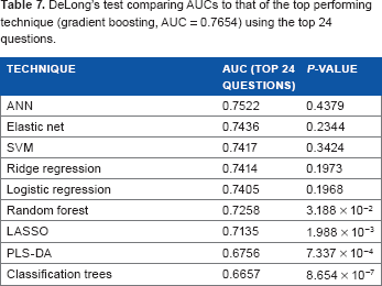
DeLong's test comparing AUCs to that of the top performing technique (gradient boosting, AUC = 0.7654) using the top 24 questions.

TECHNIQUE	AUC (TOP 24 QUESTIONS)	P-VALUE
ANN	0.7522	0.4379
Elastic net	0.7436	0.2344
SVM	0.7417	0.3424
Ridge regression	0.7414	0.1973
Logistic regression	0.7405	0.1968
Random forest	0.7258	3.188 x 10^-2
LASSO	0.7135	1.988 x 10^-3
PLS-DA	0.6756	7.337 x 10^-4
Classification trees	0.6657	8.654 x 10^-7

Table 8

Fourteen questions used in PLS-DA after removing those with zero or near zero variance from the initial 24 variables (AUC = 0.6756).

QUESTION NO.	CONTENT
90	{Do you/Does SP} now have any health problem that requires {you/him/her} to use special equipment, such as a cane, a wheelchair, a special bed, or a special telephone?
72	Including living and deceased, were any of {SP's/ your} biological that is, blood relatives including grandparents, parents, brothers, sisters ever told by a health professional that they had … osteoporosis or brittle bones?
24	{Have you/Has SP} ever received the hepatitis A vaccine series? This is a two dose vaccine that is given to people who travel outside the United States. It has only been available since 1995.
69	Including living and deceased, were any of {SP's/ your} biological that is, blood relatives including grandparents, parents, brothers, sisters ever told by a health professional that they had … Alzheimer's disease?
76	Has a doctor ever told {you/SP} that {you/s/he} had broken or fractured {your/his/her} … wrist?
42	Up to the present time, what is the most {you have/SP has} ever weighed?
6	Now I'm going to ask a few questions about milk products. Do not include their use in cooking. In the past 30 days, how often did {you/SP} have milk to drink or on {your/his/her} cereal? Please include chocolate and other flavored milks as well as hot cocoa made with milk. Do not count small amounts of milk added to coffee or tea. Would you say..
47	The next questions are about the food eaten by {you/you and your household}. {When answering these questions, think about all the people who eat here, even if they are not related to you.} Which of these statements best describes the food eaten {by you/ in your household} in the last 12 months, that is since {DISPLAY CURRENT MONTH} of last year. 1. {I/We} always have enough to eat and the kinds of food {I/we} want; 2. {I/We} have enough to eat but not always the kinds of food {I/we} want; 3. Sometimes or often {I/we} don't have enough to eat.
63	Has a doctor or other health professional ever told {you/SP} that{you/s/he} … was overweight?
71	Including living and deceased, were any of {SP's/ your} biological that is, blood relatives including grandparents, parents, brothers, sisters ever told by a health professional that they had … arthritis?
82	The next questions are about alcoholic beverages. When answering think about {your/SP's} use over the past 30 days. How often did {you/SP} drink beer or lite beer?
88	[During the past 3 months], did {you/SP} have low back pain?
107	Did {you/SP} have a stomach or intestinal illness with vomiting or diarrhea that started during those 30 days?
112	How much did {you/SP} weigh at age 25? [If you don't know {your/his/her} exact weight, please make your best guess.]

We also considered subsetting variable clusters based on the frequency of their selection by GA. Owing to the aforementioned constraints on variable inclusion in PLS-DA, it was not performed with the smaller variable subsets. Utilizing the 13 most frequently selected variables, gradient boosting still garnered the best AUC performance (AUC = 0.7371), using 10,000 trees and allowing an interaction depth of one unit as the optimum parameter. Conversely, Classification Tree was still the least optimal technique (AUC = 0.6657) (Table 6). We further subset and analyzed the top nine most frequently selected variables and found ANN as the best performing technique (AUC = 0.7154), using 50 hidden layers and a 0.04 decay parameter. ANN was also the top performing technique (AUC = 0.6714) after further downsizing to include only the five most frequently selected questions, using three hidden layers and a 0.04 decay parameter. All of our ANN analyses utilized 200 maximum iterations as the optimum parameter. Finally, our analysis using the three most frequently selected variables yielded similar AUC values with 5 out of 10 techniques, including gradient boosting, ANN, elastic net, RR, and logistic regression (AUC = 0.6629). LASSO also performed quite similarly (AUC = 0.6628), while Classification Trees again yielded the poorest performance (AUC = 0.6470) (Table 6). It should be noted that despite tuning various parameters in each of these machine learning techniques, the AUC values converged similarly to a common value of -0.6629 in 50% of all algorithms when only the three most frequently selected variables were considered.

It is also important to observe that the AUC values decrease as fewer variables are considered in the analysis, suggesting that even the variables selected less frequently by GA contribute to predictive capability. Thus, the use of all 24 selected variables allowed for the best performance overall and gradient boosting in particular provided the most accurate model.

Gradient boosting ensemble classifiers are a family of powerful machine learning techniques that have shown considerable success and flexibility in a wide range of applications.^65–68 The high flexibility of this technique can be attributed to its high degrees of freedom, which make the choice of the most appropriate loss function a matter of trial and error.⁸⁸ Thus, it is unsurprising that boosting performed so well in our study, as it has in other classification and prediction tasks.^69–73 To fully understand the current study, however, it is important to note that no machine learning technique will perform best in all settings and that even traditional statistical approaches may outperform learning algorithms in some cases.^74,75 The performance of statistical and machine learning techniques is dependent on the population and outcome of interest, the availability and dimensionality of variables,^76,77 and the criteria used to evaluate algorithm performance.⁷⁸ Consequently, studies comparing machine learning techniques for various classification and prediction tasks have produced heterogeneous results. For example, while LASSO fared relatively poorly in our study, it has performed optimally compared to other machine learning algorithms in various settings.^79–81 It has been shown, however, that LASSO provides better prediction in high-dimensional orthogonal problems with few true predictors, while RR and elastic net can effectively handle many variables with moderate predictive power.⁸⁹ Since our analysis only included variables suggested by GA to have some degree of predictive power, LASSO performance suffered while RR and elastic net had a slight advantage. The relatively accurate performance of ANN, too, may be attributed to its ability to handle complex or nonlinear relationships between variables, as are often encountered in predicting health outcomes.^82,83 Decision tree-based methods (random forests and classification trees) yielded suboptimal performance in our study, likely due to the size and complexity of the training set, which can confound tree construction and reduce node purity.⁸⁴ Classification trees performed most poorly, however, likely due to the added tendency of individual decision trees to overfit in large training sets.⁸⁵ PLS-DA, on the other hand, is capable of handling more complex problems,⁸⁶ but its performance likely suffered from the limited number of variables utilized by the technique.

The optimization of questionnaire variable selection and the ability to construct predictive models using selected variables represent a promising enterprise for researchers and clinicians alike. With techniques such as those employed in our study, interesting questions may be posed regarding the importance of variables for understanding a certain outcome, enabling rational questionnaire design and improved diagnostic or prognostic capabilities. However, independent validation is needed before such methods are integrated into everyday clinical practice. Additionally, to optimize predictive reliability, machine learning techniques must be chosen according to the characteristics of the population and variables in question, as illustrated in our study.

We also explored the interdependency of our variables by implementing a gene interaction network model in GALGO. In Supplementary Figure 4, the numerical values 1 through 7 (coded in black) represent the seven most highly ranked or most prioritized variables (questions 59, 60, 90, 72, 27, 24, and 55 represent numerical values 1-7, respectively) from our earlier GA stochastic search analyses. This figure illustrates the interdependency of these top-ranked variables, with line thickness representing the relative dependency strength. The figure suggests that the top seven questions are, for the most part, independent of each other. It is shown, however, that numerical values 3 (question 90) and 5 (question 27), and 2 (question 60) and 6 (question 24) show strong interdependence, perhaps implying that such questions may cluster together in multivariate models. Further detailed investigation and explanation regarding these interactions are the next steps to follow in this study.

Conclusion

This study provided a novel examination of GA as a useful tool for variable selection in the context of questionnaire data. From an initial set of 123 variables, GA selected 24 variables from the NHANES for use in predictive modeling of five-year mortality with machine learning techniques. This study was uniquely comprehensive in its consideration of such techniques, and gradient boosting performed most optimally (AUC = 0.7654), significantly outperforming random forest, LASSO, PLS-DA, and Classification Tree techniques (P < 0.05). Its performance, however, was not significantly different (P > 0.05) than that of ANN, elastic net, SVM, RR, or logistic regression. Insights obtained from this study can be used to design automated methods for variable selection and outcome prediction in a clinical setting. Further independent validation is needed, however, for these methods to be considered in everyday clinical practice.

Author contributions

Conceived and designed the experiments: GGD. Analyzed the data: GGD, LJA, GB. Wrote the first draft of the manuscript: GGD. Contributed to the writing of the manuscript: GGD, LJA, GB. Agree with manuscript results and conclusions: GGD, LJA, GB. Jointly developed the structure and arguments for the paper: GGD, LJA, GB. Made critical revisions and approved the final version: GGD, LJA, GB. All authors reviewed and approved the final manuscript.

supplementary Materials

supplementary Table S1. The questionnaire used in the GA procedure.

supplementary Figure 1. Sample default monitoring of accumulated chromosomes in trial 1.

supplementary Figure 2. Sample evolution of the maximum fitness across generations in 303 independent searches for trial 1.

supplementary Figure 3. Sample gene rank stability in 300 chromosomes in trial 1.

supplementary Figure 4. Sample gene interaction network within models for trial 1.

Footnotes

Acknowledgments

We would like to acknowledge the NHANES and the NDI for providing the data.

References

Fodor

I.K.

A Survey of Dimension Reduction Techniques. LLNL Technical Report, UCRL-ID-148494; 2002: 1–18.

Breiman

Random forests. Mach Learn [Internet]. 2001 [cited 2015 Feb 6]; 45(1): 5–32. Available from: http://link.springer.com/article/10.1023/A%3A1010933404324.

Yang

, Honavar

Feature subset selection using a genetic algorithm. In: Liu

, Motoda

, editors. Feature Extraction, Construction and Selection [Internet]. Berlin: Springer; 1998: 117–36 [cited 2015 Feb 6]. Available from: http://link.springer.com/chapter/10.1007/978-1-4615-5725-8_8.

Sivanandam

S.N.

, Deepa

S.N.

Introduction to Genetic Algorithms. Berlin: Springer Science & Business Media; 2007: 453.

de Oliveira

F.C.

, Borges

C.C.

, Almeida

F.N.

. SNPs selection using support vector regression and genetic algorithms in GWAS. BMC Genomics. 2014; 15(suppl 7): S4.

Gong

, Guo

, Li

, Zhu

, Lv

, Rao

. Application of a genetic algorithm - support vector machine hybrid for prediction of clinical phenotypes based on genome-wide snp profiles of sib pairs. In: Wang

, Jin

, editors. Fuzzy Systems and Knowledge Discovery [Internet]. Berlin: Springer; 2005 [cited 2015 Feb 28]. 830–5. Available from: http://link.springer.com/chapter/10.1007/11540007_103.

Mouawad

A.E.

, Mansour

Multi-marker-LD based genetic algorithm for tag SNP selection. Interdiscip Sci. 2014; 6(4): 303–11.

Mooney

, Wilmot

; Bipolar Genome Study

, McWeeney

The GA and the GWAS: using genetic algorithms to search for multilocus associations. IEEE/ACM Trans Comput Biol Bioinforma. 2012; 9(3): 899–910.

Yang

C-H

, Chuang

L-Y

, Chen

Y-J

, Tseng

H-F

, Chang

H-W

. Computational analysis of simulated SNP interactions between 26 growth factor-related genes in a breast cancer association study. OMICS. 2011; 15(6): 399–407.

10.

Chang

W-C

, Fang

Y-Y

, Chang

H-W

. Identifying association model for single-nucleotide polymorphisms of ORAI1 gene for breast cancer. Cancer Cell Int [Internet]. 2014 [cited 2015 Jul 14]; 14(1): 29. Available from: http://www.cancerci.com/content/14/1/29/abstract.

11.

Inagaki

, Haseyama

, Kitajima

A genetic algorithm for determining multiple routes and its applications. In: Proceedings of the 1999 IEEE International Symposium on Circuits and Systems, 1999 ISCAS ‘99, Vol. 6; 1999: 137–40.

12.

Jones

, Willett

, Glen

R.C.

, Leach

A.R.

, Taylor

Development and validation of a genetic algorithm for flexible docking1. J Mol Biol [Internet]. 1997 [cited 2015 Feb 28]; 267(3): 727–48. Available from: http://wvww.sciencedirect.com/science/article/pii/S0022283696908979.

13.

Wiley. Designing and Conducting Health Surveys: A Comprehensive Guide. Aday

L.A.

, Cornelius

L.J.

, eds. 3rd ed. [Internet]. [cited 2015 Jul 27]. Available from: http://www.wiley.com/WileyCDA/WileyTitle/productCd-0787975605.html.

14.

Dillman

D.A.

Mail and Internet Surveys: The Tailored Design Method - 2007 Update with New Internet, Visual, and Mixed-Mode Guide. New York City: John Wiley & Sons; 2011: 572.

15.

Kuorinka

, Jonsson

, Kilbom

. Standardised Nordic questionnaires for the analysis of musculoskeletal symptoms. Appl Ergon. 1987; 18(3): 233–7.

16.

Legault

E.P.

, Cantin

, Descarreaux

Assessment of musculoskeletal symptoms and their impacts in the adolescent population: adaptation and validation of a questionnaire. BMC Pediatr. 2014; 14: 173.

17.

Berwick

D.M.

, Murphy

J.M.

, Goldman

P.A.

, Ware

J.E.

, Barsky

A.J.

, Weinstein

M.C.

Performance of a five-item mental health screening test. Med Care. 1991; 29(2): 169–76.

18.

Knouse

L.E.

, Zvorsky

, Safren

S.A.

Depression in adults with attention-deficit/ hyperactivity disorder (ADHD): the mediating role of cognitive-behavioral factors. Cogn Ther Res [Internet]. 2013 [cited 2015 Jul 27]; 37(6): 1220–32. Available from: http://link.springer.com/article/10.1007/s10608-013-9569-5.

19.

Thapar

, Hammerton

, Collishaw

. Detecting recurrent major depressive disorder within primary care rapidly and reliably using short questionnaire measures. Br J Gen Pract. 2014; 64(618): e31–7.

20.

Rissanen

T.H.

, Voutilainen

, Virtanen

J.K.

. Low intake of fruits, berries and vegetables is associated with excess mortality in men: the Kuopio Ischaemic Heart Disease Risk Factor (KIHD) Study. J Nutr. 2003; 133(1): 199–204.

21.

Zhang

W.L.

, Lopez-Garcia

, Li

T.Y.

, Hu

F.B.

, van Dam

R.M.

Coffee consumption and risk of cardiovascular events and all-cause mortality among women with type 2 diabetes. Diabetologia [Internet]. 2009 [cited 2015 Jul 27];52(5): 810–7. Available from: http://www.ncbi.nlm.nih.gov/pmc/articles/PMC2666099/.

22.

Sali

, Roohafza

, Sadeghi

, Andalib

, Shavandi

, Sarrafzadegan

Validation of the revised stressful life event questionnaire using a hybrid model of genetic algorithm and artificial neural networks. Comput Math Methods Med. 2013; 2013: 601640.

23.

Sun

L.M.

, Chiu

H-W

, Chuang

C.Y.

, Liu

A prediction model based on an artificial intelligence system for moderate to severe obstructive sleep apnea. Sleep Breath. 2011; 15(3): 317–23.

24.

Madden

A.D.

Genetic algorithms: a pragmatic, non-parametric approach to exploratory analysis of questionnaires in educational research. Educ Res [Internet]. 1999 [cited 2015 Feb 6]; 41(2): 163–72. Available from: http://dx.doi.org/10.1080/0013188990410204.

25.

Yukselturk

, Ozekes

, Türel

Y.K.

Predicting dropout student: an application of data mining methods in an online education program. Eur J Open Distance E-Learn [Internet]. 2014 [cited 2015 Feb 7]; 17(1): 118–33. Available from: http://www.degruyter.com/view/j/eurodl.2014.17.issue-1/eurodl-2014-0008/eurodl-2014-0008.xml.

26.

McCall

Genetic algorithms for modelling and optimisation. J Comput Appl Math [Internet]. 2005 [cited 2015 Feb 28];184(1): 205–22. Available from: http://www.sciencedirect.com/science/article/pii/S0377042705000774.

27.

Whitley

A genetic algorithm tutorial. Stat Comput [Internet]. 1994 [cited 2015 Feb 28]; 4(2): 65–85. Available from: http://link.springer.com/article/10.1007/BF00175354.

28.

Goldberg

D.E.

Genetic Algorithms in Search, Optimization and Machine Learning. 1st ed. Boston, MA: Addison-Wesley Longman Publishing Co., Inc.; 1989.

29.

Gopi

ES.

Algorithm Collections for Digital Signal Processing Applications Using Matlab. Berlin: Springer Science and Business Media; 2007: 200.

30.

Anson

, Luy

Mortality in an International Perspective. Berlin: Springer Science and Business Media; 2014: 360.

31.

Amelia

I.I.

A Program for Missing Data [Internet] [cited 2015 Jan 19]. Available from: http://gking.harvard.edu/amelia/.

32.

Trevino

, Falciani

GALGO: an R package for multivariate variable selection using genetic algorithms. Bioinformatics [Internet]. 2006 [cited 2015 Jan 19]; 22(9): 1154–1156. Available from: http://bioinformatics.oxfordjournals.org/content/22/9/1154.

33.

Berglund

, Heeringa

S.G.

Multiple Imputation of Missing Data Using SAS. Cary: SAS Institute; 2014: 164.

34.

Lakany

, Conway

B.A.

Understanding intention of movement from electroencephalograms. Expert Syst [Internet]. 2007 [cited 2015 Jul 1];24(5): 295–304. Available from: http://onlinelibrary.wiley.com/doi/10.1111/j.1468-0394.2007.00435.x/abstract.

35.

Izabela Rejer

K.L.

Genetic algorithm and forward selection for feature selection in EEG feature space. J Theor Appl Comput Sci. 2013; 7(2): 72–82.

36.

Cao

B-Y

, Nasseri

Fuzzy Information and Engineering and Operations Research and Management. Berlin: Springer Science & Business Media; 2013: 558.

37.

from others GR with contributions. gbm: generalized boosted regression models [Internet]. 2015 [cited 2015 Jul 1]. Available from: http://cran.r-project.org/web/packages/gbm/index.html.

38.

Ripley

, Venables

nnet: Feed-Forward Neural Networks and Multinomial Log-Linear Models [Internet]. 2015 [cited 2015 Jul 1]. Available from: http://cran.r-project.org/web/packages/nnet/index.html.

39.

Friedman

, Hastie

, Simon

, Tibshirani

glmnet: lasso and elastic-net regularized generalized linear models [Internet]. 2015 [cited 2015 Jul 1]. Available from: http://cran.r-project.org/web/packages/glmnet/index.html.

40.

Meyer

, Dimitriadou

, Hornik

.; (libsvm C++-code). e1071: Misc Functions of the Department of Statistics (e1071), TU Wien [Internet]. 2014 [cited 2015 Jul 1]. Available from: http://cran.r-project.org/web/packages/e1071/index.html.

41.

Therneau

, Atkinson

, Ripley

(author of initial R port). rpart: Recursive partitioning and regression trees [Internet]. 2015 [cited 2015 Jul 1]. Available from: http://cran.r-project.org/web/packages/rpart/index.html.

42.

Cutler F original by LB and A, Wiener R port by AL and M. randomForest: Breiman and Cutler's random forests for classification and regression [Internet]. 2014 [cited 2015 Jul 1]. Available from: http://cran.r-project.org/web/packages/randomForest/index.html.

43.

Roever

, Raabe

, Luebke

, Ligges

, Szepannek

, Zentgraf

klaR: Classification and visualization [Internet] 2014 [cited 2015 Jul 14]. Available from: http://cran.r-project.org/web/packages/klaR/index.html.

44.

Max Kuhn. Contributions from, Wing

, Weston

, Williams

. caret: Classification and Regression Training [Internet]. 2015 [cited 2015 Jul 14]. Available from: http://cran.r-project.org/web/packages/caret/index.html.

45.

R for Mac OS X [Internet] [cited 2015 Jun 7]. Available from: http://cran.r-project.org/bin/macosx/.

46.

Buhlmann

, Hothorn

Boosting algorithms: regularization, prediction and model fitting. Stat Sci. 2007; 22(4): 477–505.

47.

Jain

A.K.

, Mao

, Mohiuddin

K.M.

Artificial neural networks: a tutorial. Computer. 1996; 29(3): 31–44.

48.

Zou

, Hastie

Regularization and variable selection via the elastic net. J R Stat Soc Ser B. 2005; 67: 301–20.

49.

Cortes

, Vapnik

Support-vector networks. Mach Learn. 1995; 20(3): 273–97.

50.

Hoerl

A.E.

, Kennard

R.W.

Ridge regression: biased estimation for nonorthogonal problems. Technometrics. 1970; 12(1): 55–67.

51.

Walker

S.H.

, Duncan

D.B.

Estimation of the probability of an event as a function of several independent variables. Biometrika [Internet]. 1967 [cited 2015 Jul 14]; 54(1-2): 167–79. Available from: http://biomet.oxfordjournals.org/content/54/1-2/167.

52.

Sulaiman

H.A.

, Othman

M.A.

, Othman

M.F.I.

, Rahim

Y.A.

, Pee

N.C.

Advanced computer and communication engineering technology. In: Proceedings of the 1st International Conference on Communication and Computer Engineering. Springer; 2014: 1063.

53.

Tibshirani

Regression shrinkage and selection via the lasso. J R Stat Soc. 1996; 58(1): 267–88.

54.

Haenlein

, Kaplan

A.M.

A beginner's guide to partial least squares analysis. Underst Stat. 2004; 3(4): 283–97.

55.

Strobl

, Malley

, Tutz

An introduction to recursive partitioning: rationale, application and characteristics of classification and regression trees, bagging and random forests. Psychol Methods. 2009; 14(4): 323–48.

56.

Fawcett

, Flach

P.A.

A response to Webb and Ting's on the application of ROC analysis to predict classification performance under varying class distributions. Mach Learn. 2005; 58(1): 33–8.

57.

Robin

, Turck

, Hainard

, Tiberti

, Lisacek

, Muller J-CS and M. pROC: Display and Analyze ROC Curves [Internet]. 2015 [cited 2015 Jul 1]. Available from: http://cran.r-project.org/web/packages/pROC/index.html.

58.

Faber

, Klaas

Estimating the uncertainty in estimates of root mean square error of prediction: application to determining the size of an adequate test set in multivariate calibration. Chemom Intell Lab Syst [Internet]. 1999 [cited 2015 Mar 29]; 49(1): 79–89. Available from: http://www.sciencedirect.com/science/article/pii/S0169743999000271.

59.

Surveillance for certain health behaviors among states and selected local areas -United States, 2010 [Internet] [cited 2015 May 16]. Available from: http://www.cdc.gov/mmwr/preview/mmwrhtml/ss6201a1.htm.

60.

fs310_2008.pdf [Internet]. [cited 2015 May 16]. Available from: http://www.who.int/mediacentre/factsheets/fs310_2008.pdf.

61.

Sun

, Lee

S.H.

, Heng

B.H.

, Chin

V.S.

5-year survival and rehospitalization due to stroke recurrence among patients with hemorrhagic or ischemic strokes in Singapore. BMC Neurol [Internet]. 2013 [cited 2015 May 16]; 13(1): 133. Available from: http://www.biomedcentral.com/1471-2377/13/133/abstract.

62.

Smajlović

, Kojić

, Sinanović

Five-year survival-after first-ever stroke. Bosn J Basic Med Sci Udruženje Basičnih Med Znan Assoc Basic Med Sci. 2006; 6(3): 17–22.

63.

Martinez

F.J.

, Foster

, Curtis

J.L.

. Predictors of mortality in patients with emphysema and severe airflow obstruction. Am J Respir Crit Care Med [Internet]. 2006 [cited 2015 May 16]; 173(12): 1326–34. Available from: http://www.atsjournals.org/doi/abs/10.1164/rccm.200510-1677OC.

64.

Whalen

, Pandey

A comparative analysis of ensemble classifiers: case studies in genomics. ArXiv13095047 Cs Q-Bio Stat [Internet]. 2013 [cited 2015 Jul 5]; Available from: http://arxiv.org/abs/1309.5047.

65.

Bissacco

, Yang

M-H

, Soatto

Fast human pose estimation using appearance and motion via multi-dimensional boosting regression. In: IEEE Conference on Computer Vision and Pattern Recognition, 2007 CVPR ‘07;2007: 1-8.

66.

Hutchinson

R.A.

, Liu

L-P

, Dietterich

T.G.

Incorporating boosted regression trees into ecological latent variable models. In: Twenty-Fifth AAAI Conference on Artificial Intelligence [Internet]. 2011 [cited 2015 Jul 14]. Available from: http://www.aaai.org/ocs/index.php/AAAI/AAAI11/paper/view/3711.

67.

Pittman

S.J.

, Brown

K.A.

Multi-scale approach for predicting fish species distributions across coral reef seascapes. PLoS One. 2011; 6(5): e20583.

68.

Johnson

, Zhang

Learning nonlinear functions using regularized greedy forest. IEEE Trans Pattern Anal Mach Intell. 2013; 36(5): 942–54.

69.

Ogutu

J.O.

, Piepho

H-P

, Schulz-Streeck

A comparison of random forests, boosting and support vector machines for genomic selection. BMC Proc. 2011; 5(suppl 3): S11.

70.

Moisen

G.G.

, Freeman

E.A.

, Blackard

J.A.

, Frescino

T.S.

, Zimmermann

N.E.

, Edwards

T.C.

Jr . Predicting tree species presence and basal area in Utah: a comparison of stochastic gradient boosting, generalized additive models, and tree-based methods. Ecol Model [Internet]. 2006 [cited 2015 Jul 20]; 199(2): 176–87. Available from: http://www.sciencedirect.com/science/article/pii/S0304380006002560.

71.

Roe

B.P.

, Yang

H-J

, Zhu

, Liu

, Stancu

, McGregor

Boosted decision trees as an alternative to artificial neural networks for particle identification. Nucl Instrum Methods Phys Res Sect Accel Spectrometers Detect Assoc Equip [Internet]. 2005 [cited 2015 Jul 20]; 543(2-3): 577–84. Available from: http://arxiv.org/abs/physics/0408124.

72.

Truccolo

, Donoghue

J.P.

Nonparametric modeling of neural point processes via stochastic gradient boosting regression. Neural Comput. 2007; 19(3): 672–705.

73.

Shi

, Paiement

, Grangier

, Yu

Learning from heterogeneous sources via gradient boosting consensus. In: Proceedings of the 2012 SIAM International Conference on Data Mining [Internet]. Society for Industrial and Applied Mathematics; 2012 [cited 2015 Jul 20]. 224–35. Available from: http://epubs.siam.org/doi/abs/10.1137/1.9781611972825.20.

74.

Kaiserman

, Rosner

, Pe'er

Forecasting the prognosis of choroidal melanoma with an artificial neural network. Ophthalmology. 2005; 112(9): 1608.

75.

Kim

Y.S.

, Sohn

S.Y.

, Kim

D.K.

, Kim

, Paik

Y.H.

, Shim

H.S.

Screening test data analysis for liver disease prediction model using growth curve. Biomed Pharmacother. 2003; 57(10): 482–8.

76.

Song

, Mitnitski

, Cox

, Rockwood

Comparison of machine learning techniques with classical statistical models in predicting health outcomes. Stud Health Technol Inform. 2004; 107(pt 1): 736–40.

77.

Guyon

, Weston

, Barnhill

, Vapnik

Gene selection for cancer classification using support vector machines. Mach Learn. 2002; 46(1-3): 389–422.

78.

Roumani

Y.F.

, May

J.H.

, Strum

D.P.

, Vargas

L.G.

Classifying highly imbalanced ICU data. Health Care Manag Sci. 2012; 16(2): 119–28.

79.

Jiménez-Montero

J.A.

, González-Recio

, Alenda

Comparison of methods for the implementation of genome-assisted evaluation of Spanish dairy cattle. J Dairy Sci. 2013; 96(1): 625–34.

80.

Ogutu

J.O.

, Schulz-Streeck

, Piepho

H-P

. Genomic selection using regularized linear regression models: ridge regression, lasso, elastic net and their extensions. BMC Proc [Internet]. 2012 [cited 2015 Jul 20];6(Suppl 2): S10. Available from: http://www.biomedcentral.com/1753-6561/6/S2/S10/abstract.

81.

Mansiaux

, Carrat

Detection of independent associations in a large epi-demiologic dataset: a comparison of random forests, boosted regression trees, conventional and penalized logistic regression for identifying independent factors associated with H1 N1pdm influenza infections. BMC Med Res Methodol [Internet]. 2014 [cited 2015 Jul 20]; 14(1): 99. Available from: http://www.biomedcentral.com/1471-2288/14/99/abstract.

82.

Liew

P-L

, Lee

Y-C

, Lin

Y-C

. Comparison of artificial neural networks with logistic regression in prediction of gallbladder disease among obese patients. Dig Liver Dis [Internet]. 2007 [cited 2015 Jul 20];39(4): 356–62. Available from: http://www.sciencedirect.com/science/article/pii/S1590865807000047.

83.

J.V.

Advantages and disadvantages of using artificial neural networks versus logistic regression for predicting medical outcomes. J Clin Epidemiol [Internet]. 1996 [cited 2015 Jun 21];49(11): 1225–31. Available from: http://www.science-direct.com/science/article/pii/S0895435696000029.

84.

Srivastava

, Han

E-H

, Singh

, Kumar

Parallel formulations of decision-tree classification algorithms. In: 1998 International Conference on Parallel Processing, 1998 Proceedings. Minneapolis, MN. 1998. 237–44.

85.

Cook

E.F.

, Goldman

Empiric comparison of multivariate analytic techniques: advantages and disadvantages of recursive partitioning analysis. J Chronic Dis. 1984; 37(9-10): 721–31.

86.

Boulesteix

A-L

, Strimmer

Partial least squares: a versatile tool for the analysis of high-dimensional genomic data. Brief Bioinform. 2007; 8(1): 32–44.

87.

Gulley

S.P.

, Rasch

E.K.

, Chan

The complex web of health: relationships among chronic conditions, disability, and health services. Public Health Rep [Internet]. 2011 [cited 2015 May 16]; 126(4): 495–507. Available from: http://www.ncbi.nlm.nih.gov/pmc/articles/PMC3115209/.

88.

Natekin

, Knoll

Gradient boosting machines, a tutorial. Front Neurorobotics [Internet]. 2013 [cited 2015 Jul 14];7. Available from: http://www.ncbi.nlm.nih.gov/pmc/articles/PMC3885826/.

89.

Waldron

, Pintilie

, Tsao

M-S

, Shepherd

F.A.

, Huttenhower

, Jurisica

Optimized application of penalized regression methods to diverse genomic data. Bioinformatics [Internet]. 2011 [cited 2015 Jul 20];27(24): 3399–406. Available from: http://bioinformatics.oxfordjournals.org/content/27/24/3399.

Development and Application of a Genetic Algorithm for Variable Optimization and Predictive Modeling of Five-Year Mortality Using Questionnaire Data

Abstract

Keywords

Introduction

Methods

Variable quality control and imputation

Genetic algorithm

Machine learning techniques

Gradient boosting

Artificial neural network

Elastic net

support vector machine

Ridge regression

Logistic regression

Random forest

LASSO regression

Partial least squares-discriminant analysis

classification trees

Assessing model performance

Results and Discussion

Conclusion

Author contributions

supplementary Materials

Footnotes

Acknowledgments

References