Robust Cancer Biomarker Identification From Matched Transcriptomic Data Via Bootstrapped Regularized Conditional Logistic Regression

Abstract

Objectives:

With the increasing application of high-throughput transcriptomic data in cancer research, identifying reliable cancer biomarkers in high-dimensional settings remains a major challenge. This study aims to systematically evaluate various regularized conditional logistic regression (CLR) methods under a matched case-control (MCC) design, focusing on their performance in variable selection, parameter estimation, and predictive accuracy. Special emphasis is placed on the importance of the matching design in reducing confounding effects and improving model interpretability.

Methods:

We utilize RNA-seq data from The Cancer Genome Atlas (TCGA), specifically datasets for liver, thyroid, and lung cancers, which include paired tumor and adjacent normal tissue samples. In our analysis, we apply 4 regularized CLR methods implemented in R packages—namely “clogitL1,” “pclogit,” “clogitLasso,” and “penalizedclr”—to analyze over 20 000 gene expression features. We evaluate the comparative performance of these methods based on metrics such as gene selection stability, predictive accuracy, and interpretability. Additionally, we employ a bootstrap resampling framework to estimate gene selection probabilities, which serve as a measure of gene importance.

Results:

Our results show that incorporating the MCC design significantly enhances feature selection performance by mitigating confounding noise. The regularized CLR models successfully identify several well-established cancer-related genes with high selection consistency and statistical significance. In contrast, models that ignore the matched design tend to miss critical biomarkers or produce excessive false positives, leading to potentially misleading interpretations.

Conclusions:

This study highlights the value of integrating a matched case-control design with regularized CLR methods for the analysis of high-dimensional transcriptomic data. The proposed analytical framework offers improved accuracy, robustness, and biological relevance, providing a practical and scalable approach for cancer genomics research. It also supports the advancement of precision medicine and translational applications.

Background

Precision medicine is an emerging medical paradigm that tailors treatment and prevention strategies to individual patients based on their genetic, molecular, and environmental profiles. With the rapid advancement of gene sequencing and high-throughput technologies, precision medicine has become a transformative trend in both clinical practice and biomedical research, particularly in oncology, endocrinology, and cardiovascular medicine. Recent studies, such as the Taiwan Precision Medicine Initiative ¹ and population-specific polygenic risk scores for Han Chinese ancestry, ² provide strong evidence for the feasibility and utility of personalized approaches in large-scale and population-specific contexts. Rather than relying on a 1-size-fits-all strategy, precision medicine aims to deliver individualized therapeutic interventions while simultaneously enabling disease prevention through early risk assessment and lifestyle-based recommendations. In this context, predictive models are used to evaluate patients’ responses to treatment, whereas prognostic models help assess the risk of disease recurrence or predict survival outcomes. Both types of models are essential for guiding therapeutic strategies and monitoring disease progression.

Traditional diagnostic methods for cancer, such as imaging and histopathological examination, are widely used in clinical practice but may be limited by insufficient information or subjective interpretation by clinicians. ³ In contrast, genetic testing and molecular profiling provide earlier and more accurate diagnoses, helping physicians design personalized treatment plans that can improve patients’ quality of life and clinical outcomes. ⁴ Conventional pathological classifications, which mainly rely on tumor size and grade, offer some diagnostic value but lack molecular-level information and have limited predictive power for drug response. By analyzing gene mutations and molecular subtypes, it becomes possible to select targeted therapies according to the specific characteristics of individual tumors, thereby improving treatment accuracy and efficacy. ⁵ Molecular subtype classification integrating multi-layer data—such as global gene expression, pathway activity, and biological functions—forms the foundation of precision medicine and reveals the heterogeneity of cancers more comprehensively. Because cancer exhibits high molecular heterogeneity and complexity, ⁶ developing accurate diagnostic models that capture its biological characteristics has become a key research topic. Large-scale cancer genomic databases such as The Cancer Genome Atlas (TCGA) provide abundant and standardized data resources that greatly facilitate the development of such models.

In cancer genomics research, the Matched Case-Control (MCC) design has been widely adopted, especially in high-dimensional data contexts, as it helps control confounding factors, improve statistical power, and enhance feature identification.^{7 -9} MCC designs match key demographic variables (eg, age and sex) to ensure comparability between cases and controls in non-study variables. In genomic studies, tumor tissues and adjacent non-tumorous tissues are commonly used as matched samples for differential expression analysis. For example, in TCGA, “normal” samples generally refer to tissue adjacent to tumors that are histologically verified as non-tumorous, or to areas of the same organ without detectable pathological changes, serving as valid reference controls. Ignoring the matched design during analysis can lead to biased estimates and reduced statistical power.^10,11

With the increasing prevalence of high-dimensional data such as transcriptomics, MCC design has become increasingly important, particularly in cancer biomarker discovery. For instance, TCGA provides gene expression data from paired tumor and normal tissues, enabling the identification of differentially expressed genes and subsequent gene enrichment and pathway analyses. ¹² In the TCGA lung adenocarcinoma dataset, 506 patients are included, 58 of whom have matched tumor and normal tissue samples spanning over 20 000 gene expression profiles. Such designs offer increased statistical power and enhanced interpretability, providing a strong foundation for high-throughput transcriptomic studies. ⁹

However, high-dimensional modeling often faces the so-called “curse of dimensionality,” where the number of variables far exceeds the number of samples, leading to model overfitting and performance degradation. ¹³ To address this issue, feature selection methods are widely used to eliminate redundant and irrelevant variables while retaining key features associated with disease states. This not only enhances predictive performance but also aids in understanding underlying biological mechanisms. Although MCC designs can improve variable selection efficiency, many studies neglect the matching structure when applying feature selection methods, resulting in decreased selection accuracy and biased outcomes.^{8 -10}

Conditional Logistic Regression (CLR) is a common statistical approach for analyzing MCC data, as it accurately estimates the relationship between covariates and disease status while accounting for matched pairs. ¹⁴ However, the application of CLR in high-dimensional data remains limited, particularly when the number of samples is small, the number of variables is large, and collinearity or noise is present—conditions that reduce the model’s ability to distinguish cases from controls. To overcome these limitations, several regularized CLR methods have been proposed, such as “clogitL1,” “pclogit,” “clogitLasso,” and “penalizedclr.”^{11,15 -17} Nonetheless, these methods have rarely been systematically compared and evaluated on real high-dimensional matched gene expression datasets. Moreover, since CLR relies on linear assumptions, its ability to discriminate between cases and controls decreases in the presence of collinearity, noise, or large-scale data. ¹⁸

This study aims to conduct a systematic comparison and analysis of various regularized CLR methods using high-dimensional transcriptomic data from 3 TCGA cancer datasets with matched designs. We evaluate each method’s performance in terms of variable selection accuracy, parameter estimation stability, and predictive ability, and apply a bootstrap resampling approach to assess the stability and biological relevance of selected genes—thereby validating their potential in cancer biomarker discovery.

The major contributions of this study are as follows: we systematically integrate and evaluate multiple existing regularized CLR methods in the context of high-dimensional MCC data and propose a comprehensive analysis framework suitable for real-world applications, encompassing data preprocessing, modeling, feature selection, and result validation. Through empirical analyses of 3 TCGA cancer datasets with matched transcriptomic samples, we identify potential differentially expressed genes and underlying biological mechanisms, aiming to provide researchers in the field of precision medicine with practical analytical tools and methodological recommendations of high reference value.

Materials and Methods

TCGA Transcriptomic Data Sources

Given The data used in this study comes from TCGA project, specifically transcriptomic data, which can be downloaded using the R package “UCSCXenaTools.” ¹⁹ The cancers studied include liver hepatocellular carcinoma (LIHC), thyroid carcinoma (THCA), and lung adenocarcinoma (LUAD). Data can be accessed via the UCSC Xena platform’s TCGA Hub database at https://tcga.xenahubs.net, with official data sourced from the TCGA project’s website: https://www.cancer.gov/ccg/research/genome-sequencing/tcga.

To provide a comprehensive overview of the data used in this study, we have added Table 1, which summarizes the sample characteristics of the 3 TCGA datasets analyzed. The table includes the total number of samples, age range, gender distribution, and the number of matched tumor–normal pairs. In addition, we report the proportion of genes (out of 20 501 genes) that follow a normal distribution under the paired-sample structure in each dataset, which was assessed using the Kolmogorov–Smirnov (KS) test. For instance, the TCGA LIHC dataset contains 370 tumor and 50 normal tissue samples, with 50 patients providing both. Each sample includes data for 20 501 genes. Our analysis focuses on these 50 paired samples, labeling tumor tissues as 1 and normal tissues as 0.

Table 1.

Summary of Sample Characteristics, Matched Tumor–Normal Pairs, and Gene Distribution in the 3 TCGA Datasets Analyzed.

Cancer type	Total samples	Age (years), mean (sd)	Gender	Matched tumor–normal pairs	% genes following normal distribution (out of 20 501)
LIHC	370	59.44 (13.52)	F: 121 (32%) M: 249 (67%)	50	99.61% (20 422/20 501)
THCA	505	47.27 (15.82)	F: 366 (72.5%) M: 135 (26.7%) NA: 4 (0.8%)	59	99.01% (20 299/20 501)
LUAD	506	65.33 (9.93)	F: 271 (54%) M: 235 (46%)	58	98.61% (20 217/20 501)

We first constructed an analytical flowchart (Figure 1) to illustrate the key components of the study. Each step depicted in the flowchart was then comprehensively described to provide clarity on the methodology and rationale underlying the analysis.

Figure 1.

Flowchart of regularized conditional logistic regression analysis.

Exploratory Feature Screening in High-Dimensional Genomics

To identify potentially relevant genes for further analysis, we first conduct a pre-screening step using the entire dataset. We apply differential expression analysis (eg, paired t-tests) across all MCC samples to select a subset of genes that show significant variation. This step aims to reduce dimensionality and focus subsequent modeling on features with a strong biological signal. Importantly, we emphasize that this pre-selection serves as part of an exploratory analysis and is not used to make direct predictive performance claims. All subsequent modeling procedures, including regularized conditional logistic regression and performance evaluation, are conducted on this fixed subset of genes using cross-validation. This allows for biologically meaningful hypothesis generation within a practical framework.

Given the high dimensionality of the original data, we begin by performing an initial feature screening to eliminate less relevant features prior to applying regularized regression. ²⁰ In Differentially expressed genes (DEGs) analysis, conducting independent hypothesis tests on numerous gene expression values poses a substantial risk of false positives. To mitigate this issue, we apply the false discovery rate (FDR) control method to correct for multiple hypothesis testing. Using the Benjamini-Hochberg (BH) procedure, ²¹ we rank the P-values obtained from paired sample t-tests in ascending order and adjust each by multiplying it by m/j, where j represents the rank of the P-value and m is the total number of independent genes tested. The resulting adjusted P-values are referred to as q-values, and FDR serves as the primary criterion for selecting differentially expressed genes. Typically, we apply an FDR threshold of <.05 for filtering.

In practice, researchers often combine FDR with fold change (FC) in gene expression between 2 groups to improve biological interpretability. By taking the base-2 logarithm of FC, we obtain log2(FC). Genes with an absolute log2(FC) value exceeding a defined threshold are generally considered for selection, highlighting those that are strongly upregulated or downregulated. Based on these criteria, we select candidate genes that meet either FDR < 0.05 or |log2(FC)| >4 for further analysis.

A double filtering strategy was applied to identify variables with both statistical significance and substantial expression differences. The absolute log2(FC) threshold was empirically chosen by considering the sample size, the regularization properties of the model, and the desired balance between sensitivity and interpretability. This threshold was set to capture approximately 100 high-confidence variables while minimizing noise from marginal effects.

Regularized Conditional Logistic Regression for Matched Case-Control Data

CLR is a statistical model used to analyze paired or stratified data, primarily to address the non-independence of observations. It is applied to study the relationship between binary outcomes and multiple predictors while controlling for confounding variables. This model is typically used in case-control studies when the data is paired or stratified. In CLR, each case is usually paired with 1 or more controls, helping to account for potential confounding factors. The model is based on conditional probability, estimating the effect of predictor variables on the outcome given certain conditions. Maximum likelihood estimation is used to estimate the model parameters, allowing for the assessment of the influence of each predictor variable on the outcome.

In this study, the real data for TCGA-specific cancers consists of 1:1 MCC pairs, thus CLR is used. In the conditional logistic function, assuming there are n samples, with n/2 patients, there are n/2 = K independent strata (patients). Each stratum (patient) contains 2 samples: 1 from normal tissue and 1 from cancerous tissue. ${\mathrm{Y}}_{\mathrm{i}\left(\mathrm{k}\right)}$ represents the outcome variable for sample i in the k-th stratum (patient), where k = 1, 2,. . ., K, and i = 1, 2. If ${\mathrm{Y}}_{\mathrm{i}(\mathrm{k})}=1$ , the sample is from the cancerous tissue; if ${\mathrm{Y}}_{\mathrm{i}(\mathrm{k})}=0$ , it is from normal tissue. Let the p gene expressions for sample i in the k-th stratum be represented as ${\mathrm{x}}_{\mathrm{i}.\left(\mathrm{k}\right)}={\left({\mathrm{x}}_{\mathrm{i}1\left(\mathrm{k}\right)},{\mathrm{x}}_{\mathrm{i}2\left(\mathrm{k}\right)},\dots ,{\mathrm{x}}_{\mathrm{ip}\left(\mathrm{k}\right)}\right)}^{\text{'}}$ , where p >> n.

The conditional logistic function can be expressed as

$$\begin{array}{l}\mathrm{logit}(\mathrm{Pr}({\mathrm{Y}}_{\mathrm{i}\left(\mathrm{k}\right)}=\mathrm{1}))=\log (\frac{\mathrm{Pr}\left({\mathrm{Y}}_{\mathrm{i}\left(\mathrm{k}\right)}=1{|\mathrm{x}}_{\mathrm{i}.\left(\mathrm{k}\right)}\right)}{1-\mathrm{Pr}\left({\mathrm{Y}}_{\mathrm{i}\left(\mathrm{k}\right)}=1{|\mathrm{x}}_{\mathrm{i}.\left(\mathrm{k}\right)}\right)})\\ ={\beta }_{0\mathrm{k}}+{\beta }^{\mathrm{T}}{\mathrm{x}}_{\mathrm{i}.\left(\mathrm{k}\right)},k=1,...,K;i=1,2.\end{array}$$

(1)

where the stratum effect is included by assigning a unique intercept ${\beta }_{0\mathrm{k}}$ to each stratum, while $\beta$ represents the effect of the predictor. The conditional logistic likelihood function for the k-th stratum (case-control pair) can be further expressed as

$$\begin{array}{c}{\mathrm{L}}_{\mathrm{k}}\left(\beta \right)=\mathrm{Pr}({\mathrm{Y}}_{1\left(\mathrm{k}\right)}=1,{\mathrm{Y}}_{2\left(\mathrm{k}\right)}=0|{\mathrm{x}}_{1.\left(\mathrm{k}\right)},{\mathrm{x}}_{2.\left(\mathrm{k}\right)},{\mathrm{Y}}_{1\left(\mathrm{k}\right)}+{\mathrm{Y}}_{2\left(\mathrm{k}\right)}=1)\\ =\frac{\mathrm{P}\left({\mathrm{Y}}_{1\left(\mathrm{k}\right)}=1{|\mathrm{X}}_{1.}\left(\mathrm{k}\right)\right)\mathrm{P}\left({\mathrm{Y}}_{2\left(\mathrm{k}\right)}=0{|\mathrm{X}}_{2\mathrm{.}}\left(\mathrm{k}\right)\right)}{\mathrm{P}\left({\mathrm{Y}}_{1\left(\mathrm{k}\right)}=1{|\mathrm{X}}_{1.}\left(\mathrm{k}\right)\right)\mathrm{P}\left({\mathrm{Y}}_{2\left(\mathrm{k}\right)}=0{|\mathrm{X}}_{2.}\left(\mathrm{k}\right)\right)+\mathrm{P}\left({\mathrm{Y}}_{1\left(\mathrm{k}\right)}=0{|\mathrm{X}}_{1.}\left(\mathrm{k}\right)\right)\mathrm{P}\left({\mathrm{Y}}_{2\left(\mathrm{k}\right)}=1{|\mathrm{X}}_{2.}\left(\mathrm{k}\right)\right)}\\ =\frac{\exp \left({\beta }^{\mathrm{T}}{\mathrm{x}}_{1.\left(\mathrm{k}\right)}\right)}{\exp \left({\beta }^{\mathrm{T}}{\mathrm{x}}_{1.\left(\mathrm{k}\right)}\right)+\exp \left({\beta }^{\mathrm{T}}{\mathrm{x}}_{2.\left(\mathrm{k}\right)}\right)},k=1,,\dots ,K\end{array}$$

(2)

The full likelihood function for the 1:1 MCC study using CLR can be written as

$$\begin{array}{c}\mathrm{L}\left(\beta \right)={\displaystyle \prod }_{\mathrm{k}=1}^{\mathrm{K}}{\mathrm{L}}_{\mathrm{k}}\left(\beta \right)\\ ={\displaystyle \prod }_{\mathrm{k}=1}^{\mathrm{K}}\frac{\exp \left({\beta }^{\mathrm{T}}{\mathrm{x}}_{1.\left(\mathrm{k}\right)}\right)}{\exp \left({\beta }^{\mathrm{T}}{\mathrm{x}}_{1.\left(\mathrm{k}\right)}\right)+\exp \left({\beta }^{\mathrm{T}}{\mathrm{x}}_{2.\left(\mathrm{k}\right)}\right)}.\end{array}$$

(3)

As stated by Breslow and Day, ¹⁰ the maximum likelihood estimates (MLEs) can be computed using the likelihood function, and this can be implemented using the “clogit” package in R. However, when the predictor variables are high-dimensional and highly correlated, the performance of MLEs may not be optimal, even under the true model (oracle model). This phenomenon will be highlighted in the simulation study. Therefore, when dealing with high-dimensional paired case-control studies, it is recommended to use regularized regression.

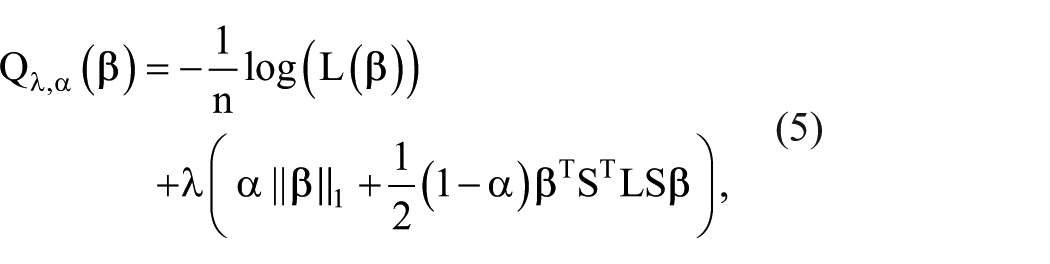
According to Reid and Tibshirani, ¹¹ the penalized conditional logistic regression model with the elastic net penalty (as defined by Zou and Hastie ²² ) is given by

$${\mathrm{Q}}_{\lambda ,\alpha }\left(\beta \right)=-\log \left(\mathrm{L}\left(\beta \right)\right)+\lambda \left(\alpha \left|\right|\beta |{|}_1+\frac{1}{2}\left(1-\alpha \right)|\left|\beta \right|{|}_2\right),$$

(4)

where $\lambda \ge 0,0\le \alpha \le 1$ , are tuning parameters to control sparsity and smoothness. We find the optimal $\beta$ estimate by minimizing the objective function ${\mathrm{Q}}_{\lambda ,\alpha }\left(\beta \right)$ . The parameter $\alpha$ specifies which penalty to use: $\alpha =0$ for Ridge; $\alpha =1$ for least absolute shrinkage and selection operator (Lasso) ²³ ; $0\le \alpha \le 1$ for Elastic Net. When $\alpha =0.5$ , it represents an equal combination of Ridge and Lasso, whereas as $\alpha \to 0$ , the penalty leans more toward Ridge, and as $\alpha \to 1$ , it leans more toward Lasso. $\lambda$ is a tuning parameter used to avoid overfitting the model to the training data. To find the optimal $(\lambda ,\alpha )$ , cross-validation can be employed. Supplemental Table S.1 summarizes the advantages and disadvantages of these 3 penalty functions.

In biological data, biomarkers are often correlated with each other, so incorporating biomarker network information into the regularized regression model can enhance the model’s effectiveness.^24,25 According to Sun and Wang, ¹⁵ the penalized conditional logistic regression likelihood with the network-based elastic net penalty function can be defined as

$$\begin{array}{c}{\mathrm{Q}}_{\lambda ,\alpha }\left(\beta \right)=-\frac{1}{\mathrm{n}}\log \left(\mathrm{L}\left(\beta \right)\right)\\ +\lambda \left(\alpha \left|\right|\beta |{|}_1+\frac{1}{2}\left(1-\alpha \right){\beta }^{\mathrm{T}}{\mathrm{S}}^{\mathrm{T}}\mathrm{LS}\beta \right),\end{array}$$

(5)

where the diagonal sign matrix ${\mathrm{S}}_{\mathrm{p*p}}=\mathrm{diag}\left({\mathrm{S}}_1,\dots ,{\mathrm{S}}_{\mathrm{p}}\right),{\mathrm{S}}_{\mathrm{u}}\in \{-1,1\}$ , represents the signs of the regression coefficients. In practice, Ridge estimators are used to calculate the estimated sign matrix. The ${\mathrm{L}}_{\mathrm{p}\mathrm{*}\mathrm{p}}$ is a symmetric adjacency matrix describing a network structure between predictors, which can include the correlation or sparse precision matrix. The sparse precision matrix can be estimated by graphical lasso,^26,27 and robust graphical lasso. ²⁸ And regression coefficient signs can improve estimates when variables within the same group or related to each other have differing signs, particularly when the coefficients are not locally smooth. Note that the “pclogit” package can perform network elastic net regularization.

Conditional Likelihood for 1:M Matched Case-Control Data

To extend the MCC design beyond the traditional 1:1 matching, we also consider the general 1:M matching structure, in which each case is matched to M controls based on covariates such as age, sex, or other potential confounders. CLR provides a natural modeling framework for analyzing such stratified data, as it accounts for the matched-set structure by conditioning out the nuisance parameters (ie, set-specific intercepts) associated with each stratum.

Let the dataset consist of K matched sets (strata), where the k-th stratum includes 1 case and M matched controls. We can derive the CLR likelihood function for 1:M matching based on the likelihood function of 1:1 matching. The complete likelihood function can be expressed as:

$$\begin{array}{c}\mathrm{L}\left(\beta \right)={\displaystyle \prod }_{\mathrm{k}=1}^{\mathrm{K}}{\mathrm{L}}_{\mathrm{k}}\left(\beta \right)\\ ={\displaystyle \prod }_{\mathrm{k}=1}^{\mathrm{K}}\frac{\exp \left({\beta }^{\mathrm{T}}{\mathrm{X}}_{1.\left(\mathrm{k}\right)}\right)}{\exp \left({\beta }^{\mathrm{T}}{\mathrm{X}}_{1.\left(\mathrm{k}\right)}\right)+{{\displaystyle \sum }}_{\mathrm{m}=2}^{\mathrm{M}+1}\exp \left({\beta }^{\mathrm{T}}{\mathrm{X}}_{\mathrm{m}.\left(\mathrm{k}\right)}\right)},\end{array}$$

(6)

The conditional log-likelihood function after taking the logarithm is

$$\begin{array}{c}\mathrm{logL}\left(\beta \right)={\displaystyle \sum }_{\mathrm{k}=1}^{\mathrm{K}}\log (\frac{\exp ({\beta }^{\mathrm{T}}{\mathbf{X}}_{1.\left(\mathrm{k}\right)})}{\exp \left({\beta }^{\mathrm{T}}{\mathbf{X}}_{1.\left(\mathrm{k}\right)}\right)+{{\displaystyle \sum }}_{\mathrm{m}=2}^{\mathrm{M}+1}\exp ({\beta }^{\mathrm{T}}{\mathbf{X}}_{\mathrm{m}.\left(\mathrm{k}\right)})})\\ ={\displaystyle \sum }_{\mathrm{k}=1}^{\mathrm{K}}({\beta }^{\mathrm{T}}{\mathbf{X}}_{1.\left(\mathrm{k}\right)}-\log \left(\begin{array}{l}\exp \left({\beta }^{\mathrm{T}}{\mathbf{X}}_{1.\left(\mathrm{k}\right)}\right)\\ +{\displaystyle \sum }_{\mathrm{m}=2}^{\mathrm{M}+1}\exp \left({\beta }^{\mathrm{T}}{\mathbf{X}}_{\mathrm{m}.\left(\mathrm{k}\right)}\right)\end{array}\right),k=1,\mathrm{2},\dots ,K\end{array}$$

(7)

This formulation removes the stratum-specific intercepts through conditioning and enables estimation of the log-odds coefficients $\beta$ , which quantify the association between covariates and the outcome, adjusting for matching. In high-dimensional settings, regularized versions of this likelihood—such as those incorporating L1 (lasso), L2 (ridge), or elastic net penalties—are commonly employed for simultaneous parameter estimation and variable selection.

Leave-One-Stratum-Out Cross-Validation (LOSOCV)

Next, the appropriate tuning parameters are identified using the leave-one-stratum-out cross-validation (LOSOCV) procedure, following van Houwelingen et al. ²⁹ Given the tuning parameters $(\alpha ,\lambda )$ , the CV error of the LOSOCV can be defined as

$$\begin{array}{l}\widehat{{\mathrm{CV}}_{\mathrm{i}}}\left(\alpha \mathrm{,}\lambda \right)=\mathrm{l}\left({\beta }_{-\mathbf{i}}\left(\alpha \mathrm{,}\lambda \right)\right)\\ -{\mathrm{l}}_{-\mathrm{i}}\left({\beta }_{-\mathbf{i}}\left(\alpha \mathrm{,}\lambda \right)\right),\mathrm{i}=1,\dots ,\mathrm{K},\end{array}$$

(8)

where ${\mathrm{l}}_{-\mathrm{i}}$ is the log-likelihood excluding the i-th stratum of the data and ${\beta }_{-\mathbf{i}}\left(\alpha ,\lambda \right)$ is obtained by using K-1 strata data. Finally, we choose the optimal $\left(\alpha ,\lambda \right)$ that maximizes ${\displaystyle \sum }_{\mathrm{i}}\widehat{{\mathrm{CV}}_{\mathrm{i}}}\left(\alpha ,\lambda \right)$ . It is important to note that in matched case-control study data, strata (patients) are independent of each other, but observations within a stratum (patient) are correlated. Therefore, when performing LOSOCV, we remove a stratum (case) rather than a single observation.

Prediction Using the Mean Method

The conditional logistic regression model eliminates the intercept interference parameters, but the parameters are crucial for predicting new data. Therefore, as per Reid and Tibshirani, ¹¹ we use 2 methods for prediction. The dataset is partitioned into training and test sets, with 70% assigned to the training set and 30% to the test set. Using the training data, the best model for each method is fitted with the LOSOCV procedure, and the estimated $\beta$ coefficients for each method are obtained. For each data point in the training set, the feature vector is multiplied by the estimated $\beta$ coefficients to obtain the linear predictor ${\widehat{\beta }}^{\mathrm{T}}{\mathbf{x}}_{\mathrm{i}.\left(\mathrm{k}\right)}$ .

The average of all the linear predictors in the training set is then computed to form a threshold. For each data point in the test set, the feature vector is multiplied by the estimated $\beta$ coefficients to calculate its linear predictor. If the linear predictor exceeds the threshold, the result is classified as a case, otherwise, it is classified as a control.

Prediction Using the Majority Voting Method

Using the training data, the best model for each method is fitted with the LOSOCV procedure, and the estimated $\beta$ coefficients for each method are obtained. For each data point in the training set, the feature vector is multiplied by the estimated $\beta$ coefficients to obtain the linear predictor. For each test data point, the linear predictor is calculated for each model, and if the linear predictor exceeds the linear predictors from more than half of the training set models, the result is classified as a case; otherwise, it is classified as a control.

These 2 forecasting methods can also be naturally extended to 1:M matched case-control design. For example, in the mean method, we first calculate the average of M linear predictors for each stratum of the M controls in the training set, and then average them with the linear predictors of the case group in the training set to form a threshold. In the majority voting method, if the linear predictor from the testing set model exceeds 100*(M/(1 + M))% of the linear predictors from the training set model, the result is classified as a case; otherwise, it is classified as a control.

Finally, a confusion matrix is created based on the test set predictions, and prediction metrics (such as G-mean and AUC) are computed for each method. It is important to note that the G-mean is a comprehensive metric that considers both sensitivity and specificity, that is, the square of the product of sensitivity and specificity, while the receiver operating characteristic curve and the corresponding area under the curve are used to adjust the penalty tuning parameters. ¹¹ In addition to comparing model prediction performance, we can also evaluate variable selection (G-mean) and parameter estimation (root mean squared error, RMSE) performance using simulated data.

Real Data Analysis for Gene Importance

In real data analysis, we first identify the best regularization condition logistic regression method for a specific cancer using the flowchart in Figure 1. Then, we apply the bootstrap method to randomly sample the 50% entire dataset (using strata as the sampling unit), perform variable selection using the best regularized CLR method, and repeat this process 100 times. This results in calculating the frequency selection probability for each gene. The probability is then used to define the gene importance. ¹⁷ We note that this bootstrap method is flexible and robust, making it less susceptible to the influence of specific samples. In other words, different samples may lead to the selection of highly different genetic combinations. The bootstrap method can alleviate this issue, resulting in more accurate biomarkers.

Summarizing the Research

Currently, there are 4 R packages (“clogitL1,” “pclogit,” “clogitLasso,” “penalizedclr”) available for performing penalized CLR (Lasso, Ridge, Elastic Net). These 4 R packages are summarized in Table 2. We have established a related workflow for this research topic.

Table 2.

Reviews on Regularized Conditional Logistic Regression (a Partial List).

R package	Description	Penalty	LOSOCV	1:1(M) matching	Citation
clogitL1	Tools designed for fitting and cross-validating exact conditional logistic regression models with lasso, ridge, and elastic net penalties. They employ cyclic coordinate descent, warm starts, and sequential strong rules to efficiently calculate the full solution path.	Lasso, Ridge, Elastic net	The built-in program in package “clogitL1” includes this procedure.	Yes	Reid and Tibshirani 11
pclogit	An efficient algorithm for fitting the regularization path and determining the selection probabilities of each predictor, designed for the analysis of high-dimensional matched (or unmatched) case-control data. It utilizes cyclical coordinate descent in a pathwise approach.	Lasso, Ridge, Elastic net, Network elastic net	The built-in program in package “pclogit” does not include this procedure; we need to write the program ourselves.	Yes	Sun and Wang 15
clogitLasso	The sequence of models suggested by the fraction is fitted using the iteratively reweighted least squares algorithm, along with cyclical coordinate descent employing warm starts and sequential strong rules.	Lasso	The built-in program in package “pclogitLasso” does not include this procedure; we need to write the program ourselves.	Yes	Avalos et al 16
penalizedclr	This method applies L1 and L2 penalized conditional logistic regression with penalty factors, facilitating the integration of various data sources. Additionally, it features stability selection for variable selection.	Lasso, Ridge, Elastic net	The built-in program in package “penalizedclr” does not include this procedure; we need to write the program ourselves.	Yes	Djordjilović et al 17

The first research objective is to conduct a systematic comparison and analysis of the penalized conditional logistic regression methods in these 4 R packages, evaluating criteria including variable selection, parameter estimation, and model predictive performance. Next, we will demonstrate through a series of simulation studies that, in high-dimensional matched case-control studies, the penalized CLR method is more effective than traditional maximum likelihood estimator and penalized ordinary logistic regression. A comprehensive statistical analysis will be performed, with the goal of providing biologists with a better understanding of current regularized conditional logistic regression methods. Finally, the study will focus on MCC study data from the TCGA project, specifically concerning LUAD, LIHC, and THCA.

Finally, we state that the reporting of this study conforms to the Strengthening the Reporting of Observational Studies in Epidemiology (STROBE) Statement (STROBE_checklist_v4_combined). The completed STROBE checklist has been submitted as a Supplemental File.

Results

Simulation Studies: Synthetic Dataset

Following the simulation framework of Sun and Wang, ¹⁵ we constructed a 1:1 MCC dataset consisting of 150 strata of data. Among them, 100 strata were used for training and 50 strata for testing. Each individual had 2000 variables. The dependent variable Y was binary, with cases coded as 1 and controls as 0. To mimic biological signal heterogeneity, we specified different mean vectors for cases and controls:

$${\mu }_{\mathrm{case}}={\left(-2_2,2_3,0_5,2_2,-2_3,0_5,-2,2_2,-2_2,0_{1975}\right)}^{/};$$

$${\mu }_{\mathrm{control}}={\left(0_{2000}\right)}^{/}.$$

The case and control means differ on specific subsets of variables to represent signal regions, similar to the settings described in Sun and Wang, ¹⁵ who generated high-dimensional MCC methylation datasets with 1000 CpG sites for computational feasibility and to maintain consistency with their simulation design.

Additionally, the stratum-level variable $\mathrm{Z}$ was generated from Beta distributions with parameters $\left(a,b\right)\in \{\left(0.5,0.5\right),\left(1,1\right),(2,2)\}$ to model heterogeneous stratum effects, following the idea of introducing varying stratum-level scaling effects. For each stratum, all data were multiplied by $\sqrt{Z}$ to incorporate stratum-specific variance scaling. Supplemental Figure S.1 shows the probability density function plots of different Beta distributions. For Beta(.5, .5), the distribution has a U-shape, with higher probabilities at 0 and 1, and lower in the middle. For Beta(1, 1), the distribution is flat, meaning the probability is the same across the entire range from 0 to 1. For Beta(2, 2), the distribution is symmetric and bell-shaped, with the highest probability around .5. Each beta distribution shows a different pattern of concentration.

We assumed that the independent variable $X_i,i=1,\dots ,150$ follows a conditional normal distribution given $Y_i$ and $Z_i=z$ , that is,

$$X_i|Y_i=1,Z_i=\mathrm{z}~\sqrt{\mathrm{z}}{N}_p\left({\mu }_{\mathrm{case}},\Sigma \right);$$

$$X_i|Y_i=0,Z_i=\mathrm{z}~\sqrt{\mathrm{z}}{N}_p\left({\mu }_{\mathrm{control}},\Sigma \right).$$

where $\Sigma$ was the covariance matrix generated from network-based structures. The covariance (or network) structures were simulated using the R package “huge” and its function huge.generator(), ³⁰ which allows the creation of multivariate Gaussian data with predefined network topologies. Four different network structures were considered:

Hub: A central node is connected to multiple other variables, forming a Hub structure.

Band: Variables are connected in a band-like structure.

Cluster: Variables form multiple clusters, with high correlations within each cluster.

Scale-free: The connections between variables follow a scale-free network characteristic, where a few variables have many connections, while others have fewer.

Figure 2 shows the 4 variable network structures. These network patterns and data distributions follow common settings in network-based high-dimensional simulation studies,^15,30 providing a controlled environment to evaluate the proposed method under varying dependency structures.

Figure 2.

The 4 gene network structures.

Considering the limited number of strata, after the initial feature selection (FDR < 0.05 or |log2(FC)| > 4), we controlled the number of features to approximately 100 and then explored several approaches. First, we considered MLE within the CLR framework, which can be implemented using the “clogit” R package. Additionally, we evaluated the penalized logistic regression method, which does not account for the paired structure of the data, and can be performed using the “glmnet” R package. We also examined 4 R packages specifically designed for penalized CLR: “clogitL1,” “pclogit,” “clogitLasso,” and “penalizedclr.” Finally, in our simulation study, we incorporated the oracle estimator, ³¹ which provides the MLE under the true model.

To investigate whether commonly used multiple testing procedures, such as the BH method, can effectively control the FDR under an MCC design, we conducted a simulation study mimicking the high-dimensional structure of gene expression data. In each simulated dataset, 2000 features were generated, of which only 15 were truly differentially expressed between matched cases and controls, while the remaining features followed the null distribution. Paired t-tests were applied to each feature to obtain P-values, and the BH procedure was subsequently used to control the FDR at a nominal level of .05. Features with adjusted q-values below 0.05 were considered significant. To estimate the empirical FDR, we calculated the proportion of false positives (null features incorrectly declared significant) among all selected features. This procedure was repeated 200 times, and the average empirical FDR was calculated across all simulations (see Supplemental Table S.2 for details). The results suggest that the BH procedure provides reasonable control of the FDR under the MCC design, with the observed empirical FDR remaining close to the target level of 0.05. These findings support the practical use of FDR-based thresholds for variable selection in high-dimensional matched-pair transcriptomic analyses.

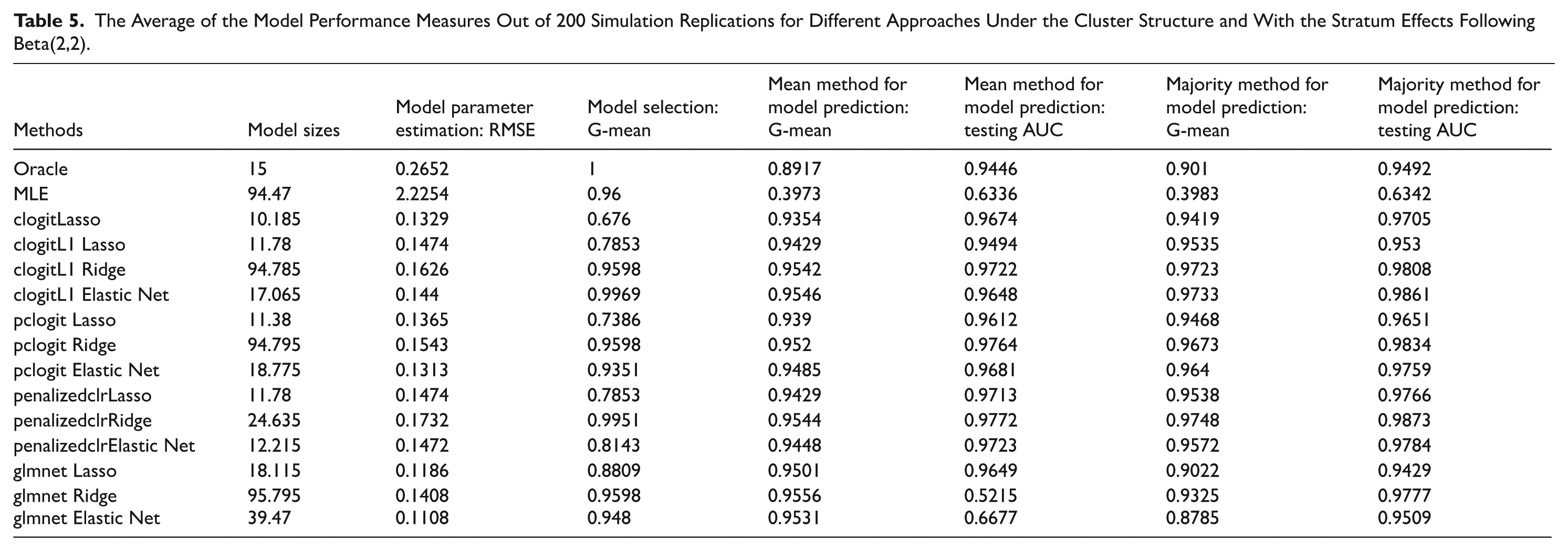
We take the average of the model performance measures out of 200 simulation replications. Based on the simulation results (Tables 3–5 and Supplemental Tables S.3–S.11), we draw several key conclusions. First, penalized CLR outperforms traditional maximum likelihood estimation in terms of parameter estimation and predictive accuracy, even in the ideal oracle estimation scenario, where the true model is known. Therefore, when there is a network structure among the features, it is recommended to use regularized regression. Second, penalized CLR outperforms penalized ordinary logistic regression in terms of predictive accuracy. Ordinary logistic regression ignores the paired structure of the data. Third, predictive accuracy varies with different levels of stratum effects, indicating that a larger beta distribution parameter value for the stratum effects leads to higher predictive accuracy. Finally, among the 4 penalized CLR R packages tested, the “penalizedclr” package demonstrated the most stable performance. It consistently provided reliable results, regardless of changes in stratum effects or network structures, making it the most robust choice across different simulation settings. Additionally, the “pclogit” package also delivered satisfactory results in terms of predictive accuracy.

Table 3.

The Average of the Model Performance Measures Out of 200 Simulation Replications for Different Approaches Under the Cluster Structure and With the Stratum Effects Following Beta(.5,.5).

Methods	Model sizes	Model parameter estimation: RMSE	Model selection: G-mean	Mean method for model prediction: G-mean	Mean method for model prediction: testing AUC	Majority method for model prediction: G-mean	Majority method for model prediction: testing AUC
Oracle	15	2.3936	1	0.6025	0.7806	0.6244	0.7903
MLE	92.745	7.6014	0.9608	0.2892	0.5482	0.2939	0.5522
clogitLasso	5.855	0.4016	0.3696	0.7255	0.8566	0.7464	0.864
clogitL1 Lasso	6.2	0.2533	0.4123	0.7383	0.8659	0.7625	0.8737
clogitL1 Ridge	93.91	0.1627	0.9602	0.7852	0.8883	0.8326	0.9071
clogitL1 Elastic Net	20.24	0.1905	0.8645	0.7761	0.8788	0.8153	0.9125
pclogit Lasso	8.845	0.2459	0.4365	0.7281	0.8667	0.7435	0.8737
pclogit Ridge	93.915	0.1524	0.9602	0.7816	0.8913	0.821	0.9049
pclogit Elastic Net	13.3	0.2321	0.5306	0.7359	0.8706	0.7502	0.8784
penalizedclrLasso	6.195	0.2536	0.412	0.7379	0.8638	0.7621	0.873
penalizedclrRidge	26.61	0.1732	0.9942	0.7858	0.8927	0.8379	0.9154
penalizedclrElastic Net	12.35	0.2382	0.7218	0.767	0.8815	0.7992	0.894
glmnet Lasso	18.005	0.1404	0.8492	0.7798	0.8666	0.7802	0.8292
glmnet Ridge	94.915	0.1444	0.9602	0.7905	0.5	0.7496	0.8987
glmnet Elastic Net	34.555	0.1393	0.9361	0.7863	0.5	0.7697	0.8482

Table 4.

The Average of the Model Performance Measures Out of 200 Simulation Replications for Different Approaches Under the Cluster Structure and With the Stratum Effects Following Beta(1,1).

Methods	Model sizes	Model parameter estimation: RMSE	Model selection: G-mean	Mean method for model prediction: G-mean	Mean method for model prediction: testing AUC	Majority method for model prediction: G-mean	Majority method for model prediction: testing AUC
Oracle	15	0.8152	1	0.7373	0.8602	0.7483	0.8651
MLE	93.645	4.1262	0.9604	0.3257	0.575	0.3273	0.5762
clogitLasso	7.47	0.1686	0.4923	0.8413	0.9188	0.8645	0.9298
clogitL1 Lasso	9.37	0.1416	0.6247	0.8588	0.9154	0.8872	0.9261
clogitL1 Ridge	93.985	0.1626	0.9602	0.8831	0.937	0.9285	0.9593
clogitL1 Elastic Net	17.57	0.1291	0.9853	0.8796	0.9297	0.9274	0.9636
pclogit Lasso	9.61	0.1502	0.5456	0.8416	0.922	0.8656	0.9338
pclogit Ridge	94	0.1533	0.9602	0.8804	0.941	0.9227	0.9602
pclogit Elastic Net	17.825	0.1404	0.7245	0.8544	0.9275	0.8838	0.9433
penalizedclrLasso	9.36	0.1416	0.624	0.8589	0.9284	0.8871	0.9418
penalizedclrRidge	25.24	0.1732	0.9948	0.883	0.9414	0.9317	0.9652
penalizedclrElastic Net	11.225	0.1374	0.7457	0.8702	0.9346	0.9021	0.9498
glmnet Lasso	18.11	0.1292	0.8856	0.8807	0.9257	0.8765	0.888
glmnet Ridge	95	0.1413	0.9602	0.8895	0.5004	0.8782	0.9552
glmnet Elastic Net	33.47	0.1269	0.9466	0.885	0.5068	0.8565	0.9017

Table 5.

The Average of the Model Performance Measures Out of 200 Simulation Replications for Different Approaches Under the Cluster Structure and With the Stratum Effects Following Beta(2,2).

Methods	Model sizes	Model parameter estimation: RMSE	Model selection: G-mean	Mean method for model prediction: G-mean	Mean method for model prediction: testing AUC	Majority method for model prediction: G-mean	Majority method for model prediction: testing AUC
Oracle	15	0.2652	1	0.8917	0.9446	0.901	0.9492
MLE	94.47	2.2254	0.96	0.3973	0.6336	0.3983	0.6342
clogitLasso	10.185	0.1329	0.676	0.9354	0.9674	0.9419	0.9705
clogitL1 Lasso	11.78	0.1474	0.7853	0.9429	0.9494	0.9535	0.953
clogitL1 Ridge	94.785	0.1626	0.9598	0.9542	0.9722	0.9723	0.9808
clogitL1 Elastic Net	17.065	0.144	0.9969	0.9546	0.9648	0.9733	0.9861
pclogit Lasso	11.38	0.1365	0.7386	0.939	0.9612	0.9468	0.9651
pclogit Ridge	94.795	0.1543	0.9598	0.952	0.9764	0.9673	0.9834
pclogit Elastic Net	18.775	0.1313	0.9351	0.9485	0.9681	0.964	0.9759
penalizedclrLasso	11.78	0.1474	0.7853	0.9429	0.9713	0.9538	0.9766
penalizedclrRidge	24.635	0.1732	0.9951	0.9544	0.9772	0.9748	0.9873
penalizedclrElastic Net	12.215	0.1472	0.8143	0.9448	0.9723	0.9572	0.9784
glmnet Lasso	18.115	0.1186	0.8809	0.9501	0.9649	0.9022	0.9429
glmnet Ridge	95.795	0.1408	0.9598	0.9556	0.5215	0.9325	0.9777
glmnet Elastic Net	39.47	0.1108	0.948	0.9531	0.6677	0.8785	0.9509

This study further explores 1:M MCC data, expanding the simulated synthetic data to a 1:4 MCC dataset. A simulation analysis is conducted under a cluster structure with 3 different stratum effect distributions (Beta(.5,.5), Beta(1,1), Beta(2,2)). Table 6 and Supplemental Tables S.12 and S.13 present the average results from 100 repeated runs under the cluster structure with the 3 different stratum effect distributions, leading to similar conclusions as the previous 1:1 MCC dataset.

Table 6.

The Average of the Model Performance Measures Out of 100 Simulation Replications for Different Approaches Under the Cluster Structure and With the Stratum Effects Following Beta(2,2) under 1:4 Matched Case-Control Study.

Methods	Model sizes	Model parameter estimation: RMSE	Model selection: G-mean	Mean method for model prediction: G-mean	Mean method for model prediction: testing AUC	Majority method for model prediction: G-mean	Majority method for model prediction: testing AUC
Oracle	15	0.2434	1	0.9272	0.9631	0.9323	0.9656
MLE	114.3301	0.2704	0.95	0.865	0.9302	0.8275	0.9116
clogitLasso	11.7184	0.1224	0.7786	0.9389	0.9691	0.9537	0.9765
clogitL1 Lasso	13.3495	0.1422	0.89	0.9454	0.9533	0.9641	0.9613
clogitL1 Ridge	114.301	0.1599	0.95	0.9542	0.9723	0.9762	0.983
clogitL1 Elastic Net	16.534	0.1392	0.9992	0.9549	0.9655	0.9761	0.9879
pclogit Lasso	13.6311	0.1518	0.9087	0.946	0.8673	0.9646	0.8697
pclogit Ridge	114.3301	0.1635	0.95	0.9517	0.9757	0.9747	0.9875
pclogit Elastic Net	14.4466	0.1472	0.9631	0.9495	0.8761	0.9688	0.8794
penalizedclrLasso	13.3495	0.1422	0.89	0.9454	0.9724	0.9641	0.9818
penalizedclrRidge	23.0777	0.1732	0.9959	0.9559	0.9779	0.9762	0.9879
penalizedclrElastic Net	13.4757	0.142	0.8984	0.9467	0.9731	0.9646	0.982
glmnet Lasso	23.5437	0.1087	0.9488	0.9499	0.9661	0.9575	0.9682
glmnet Ridge	115.3301	0.1383	0.95	0.954	0.5195	0.9715	0.9828
glmnet Elastic Net	39.7573	0.1064	0.9655	0.952	0.661	0.955	0.9744

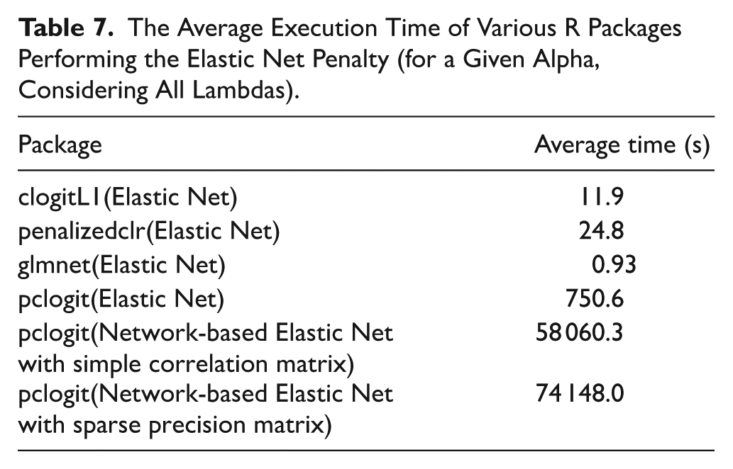
However, when using “pclogit” to run the network-based elastic net, we find that its statistical effectiveness is no better than simply running the elastic net. Additionally, the execution time is quite long. Table 7 presents the average execution time of various R packages performing the (network-based) elastic net penalty (for a given alpha, with all lambdas considered). Due to the concern about execution time, we decided not to proceed with the network-based elastic net.

Table 7.

The Average Execution Time of Various R Packages Performing the Elastic Net Penalty (for a Given Alpha, Considering All Lambdas).

Package	Average time (s)
clogitL1(Elastic Net)	11.9
penalizedclr(Elastic Net)	24.8
glmnet(Elastic Net)	0.93
pclogit(Elastic Net)	750.6
pclogit(Network-based Elastic Net with simple correlation matrix)	58 060.3
pclogit(Network-based Elastic Net with sparse precision matrix)	74 148.0

For completeness, we also implemented a network-based elastic net model using the “pclogit” package, which combines an L1 penalty with a network smoothness term to incorporate correlations among predictors. However, this approach required substantially longer execution time and yielded limited improvement in predictive performance compared to the standard elastic net model. Therefore, it was not pursued further in the main analysis. Nevertheless, the method is briefly discussed for its theoretical value and potential applicability in future studies where biologically meaningful network structures can be more accurately defined.

In this study, we focused on 3 cancer types, LIHC, THCA and LUAD, because they have relatively large sample sizes in TCGA with matched tumor and normal tissue samples, represent different organ systems and biological characteristics, and are known to exhibit substantial gene expression differences. These features make them particularly suitable for differential expression analysis and model validation. Based on the KS test results reported in Table 1, approximately 99% of genes in the 3 TCGA 1:1 matched tumor–normal datasets were normally distributed, indicating that most gene expression changes are suitable for subsequent data analysis using paired t-tests.

Real Data Application: TCGA LIHC Data

Our analysis focuses on a subset of the TCGA LIHC dataset, which includes data from 50 patients and 20 501 gene expression markers, with both normal and tumor tissue samples provided for each patient. Since the number of genes likely associated with cancer is expected to be limited, we reduce the gene count before performing the training/test split for cross-validation. We adopted a double filtering procedure, ³² where genes are first filtered based on FDR results, and then further filtered based on the magnitude of log2(FC) changes. A well-known visualization tool in genomics for illustrating the results of double filtering (based on both statistical significance and fold change) is the volcano plot, which is widely used to visualize the results of genomic experiments. A volcano plot is a scatter plot that illustrates the relationship between –log10(q) and log2(FC). As shown in Figure 3, the most strongly upregulated or downregulated features located at the extremes of the X-axis, and the most statistically significant features at the top. The findings in the upper-left and upper-right corners are typically considered the most likely to be significantly differentially expressed genes. Using this double filtering process, we considered genes to be significant if they met both FDR < 0.05 and |log2FC| > 4. This approach identified 96 candidate genes for further analysis in the LIHC dataset. However, if only 1 of the 2 conditions is required to be satisfied, the number of selected genes increases to 11 022, which is too large and unsuitable for subsequent regularization analysis.

Figure 3.

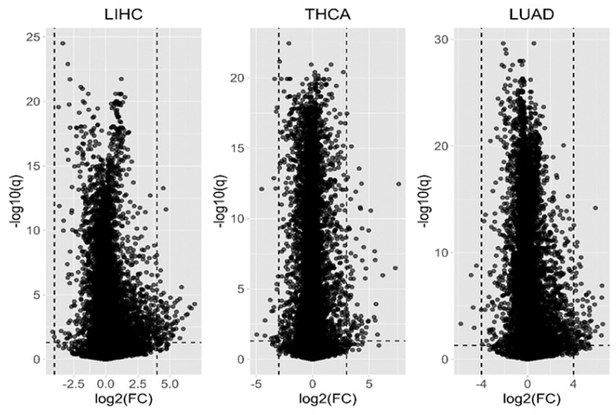
The volcano plots of TCGA LIHC, THCA, and LUAD.

We conducted 10 random splits, partitioning the entire dataset into a 7:3 training/test ratio, to assess the performance of all methods applied to the TCGA LIHC data. Using the 96 candidate genes selected through the double filtering procedure, we developed prediction models for each method. The average classification results for each method across the 10 random splits are shown in Table 8. The results show that the “pclogit” package with the ridge penalty performed best in the majority prediction method, while the elastic net penalty also performed well in both prediction methods. Since ridge does not allow for further variable selection, we used the well-performing elastic net method for the subsequent analysis. Then, we apply the bootstrap method to randomly sample 50% of the entire dataset (using strata as the sampling unit), perform variable selection using the “pclogit” with the elastic net penalty, and repeat this process 100 times. The selection frequency probability for each gene is calculated to define the importance of the gene, and a threshold of .5 is used, meaning that a gene must have a selection probability greater than .5 to be included in our final candidate model. Next, we apply the “pclogit” package with the elastic net penalty to the entire dataset and determine the optimal tuning parameters $\left(\alpha ,\lambda \right)$  = (0.35, 0.00013). Using these tuning parameters, we identify 10 important genes and obtained the corresponding parameter estimates, as presented in Table 9.

Table 8.

Results (Average of Model Performance Measures) of Different Methods on the TCGA LIHC Data Over 10 Random Splits of 7:3 Training/Test Sets After Applying Double Filtering Procedure.

Methods	Model sizes	Mean method for model prediction: G-mean	Mean method for model prediction: testing AUC	Majority method for model prediction: G-mean	Majority method for model prediction: testing AUC
MLE	55.6	0.3696	0.6431	0.3667	0.6432
clogitLasso	10.3	0.7667	0.8834	0.9408	0.97
clogitL1 Lasso	9.9	0.7667	0.8315	0.9279	0.8881
clogitL1 Ridge	96	0.72	0.7902	0.9733	0.9505
clogitL1 Elastic Net	44.7	0.7667	0.8313	0.9733	0.9868
pclogit Lasso	11.9	0.8733	0.9054	0.9214	0.8552
pclogit Ridge	96	0.7333	0.8611	0.9933	0.9967
pclogit Elastic Net	17.6	0.9	0.9252	0.9337	0.9139
penalizedclrLasso	9.8	0.7667	0.8834	0.9279	0.9633
penalizedclrRidge	79	0.54	0.7699	0.9344	0.9668
penalizedclrElastic Net	9.9	0.7667	0.8834	0.9279	0.9633
glmnet Lasso	11.4	0.7133	0.8279	0.9344	0.8952
glmnet Ridge	97	0.6667	0.5053	0.98	0.9688
glmnet Elastic Net	19.3	0.7333	0.5666	0.9604	0.9073

Table 9.

In the TCGA LIHC Dataset, Perform 100 Bootstrap Iterations to Calculate Gene Selection Probabilities, Retain Genes With Probabilities > .5, and Apply Elastic Net Penalty From “pclogit” to Estimate the Parameters.

Gene	Selected probability	Parameter estimation	Citation
SLCO1C1*	.95	1.5203
EBF2*	.9	1.2314	Ouyang et al 33
LOC221122	.7	0.6892
CELF3	.6	1.7941	Nasiri-Aghdam et al 34
KRTAP5.5	.59	0.8952
COX7B2*	.58	0.4839
B4GALNT2*	.53	0.3865
BANF2	.53	0.3449
PAEP*	.53	0.2748	Wang and Kong 35
CSMD1	.51	0.3385	Zhang et al 36

*

Genes identified by both regularized CLR and unmatched LASSO models.

Among these 10 important identified genes, several have been proven in the literature to be related to liver cancer development or cancer genesis mechanisms. Ouyang et al ³³ demonstrated that the EBF2 gene is a DEG and is upregulated in LIHC. Nasiri-Aghdam et al ³⁴ found that CELF family members are linked to cancer proliferation and invasion, being potential tumor suppressors or oncogenes. The review highlights CELF protein regulation mechanisms and their role in cancer physiology. PAEP is one of the key genes identified in the study, ³⁵ linked to angiogenesis and ferroptosis in hepatocellular carcinoma (HCC). It may serve as a potential biomarker for prognosis and immunotherapy response in HCC patients. Zhang et al ³⁶ demonstrated that CSMD1 is linked to the stage and grade of alcohol-related HCC (HCC-A) and is associated with poorer disease-free survival. It may serve as a potential biomarker for predicting survival in HCC-A patients and contribute to disease progression.

Real Data Application: TCGA THCA Data

Our analysis focuses on a subset of the TCGA THCA dataset, which includes data from 59 patients and 20 501 gene expression markers, with both normal and tumor tissue samples provided for each patient. Since the number of genes likely associated with cancer is expected to be limited, we adopted a double filtering procedure, ³² where genes are first filtered based on FDR results, and then further filtered based on the magnitude of log2(FC) changes. Using this double filtering process, we considered genes to be significant if they met both FDR < 0.05 and |log2FC| > 3. This approach identified 103 candidate genes for further analysis in the THCA dataset. However, if only 1 of the 2 conditions is required to be satisfied, the number of selected genes increases to 13 188, which is too large and unsuitable for subsequent regularization analysis.

We conducted 10 random splits, partitioning the entire dataset into a 7:3 training/test ratio, to assess the performance of all methods applied to the TCGA THCA data. Using the 103 candidate genes selected through the double filtering procedure, we developed prediction models for each method. The average classification results for each method across the 10 random splits are shown in Table 10. The results show that the “pclogit” package with the elastic net penalty performed best in both prediction methods. Then, we apply the bootstrap method to randomly sample 50% of the entire dataset, perform variable selection using “pclogit” with the elastic net penalty, and repeat this process 100 times. The selection frequency probability for each gene is calculated to define the importance of the gene, and a threshold of .5 is used, meaning that a gene must have a selection probability greater than .5 to be included in our final candidate model. Next, we apply the “pclogit” package with the elastic net penalty to the entire dataset and determine the optimal tuning parameters $\left(\alpha ,\lambda \right)$  = (0.25, 0.00014). Using these tuning parameters, we identify 20 important genes and obtained the corresponding parameter estimates, as presented in Table 11.

Table 10.

Results (Average of Model Performance Measures) of Different Methods on the TCGA THCA Data Over 10 Random Splits of 7:3 Training/Test Sets After Applying Double Filtering Procedure.

Methods	Model sizes	Mean method for model prediction: G-mean	Mean method for model prediction: testing AUC	Majority method for model prediction: G-mean	Majority method for model prediction: testing AUC
MLE	60.6	0.2357	0.5751	0.2459	0.564
clogitLasso	6.3	0.8691	0.9333	0.8972	0.9471
clogitL1 Lasso	6.7	0.8691	0.8903	0.8867	0.9053
clogitL1 Ridge	103	0.8278	0.893	0.9237	0.9179
clogitL1 Elastic Net	42.4	0.8556	0.898	0.9452	0.9608
pclogit Lasso	9.1	0.9237	0.9467	0.934	0.9496
pclogit Ridge	103	0.85	0.925	0.9667	0.9874
pclogit Elastic Net	15.2	0.9452	0.962	0.9556	0.9608
penalizedclrLasso	6.7	0.8691	0.9334	0.8867	0.9416
penalizedclrRidge	55.8	0.7944	0.8971	0.8402	0.9166
penalizedclrElastic Net	10.9	0.8583	0.9278	0.9077	0.9528
glmnet Lasso	10.9	0.9017	0.9139	0.9667	0.9323
glmnet Ridge	104	0.8	0.5927	0.8919	0.9226
glmnet Elastic Net	13.6	0.8963	0.8528	0.9667	0.9342

Table 11.

In the TCGA THCA Dataset, Perform 100 Bootstrap Iterations to Calculate Gene Selection Probabilities, Retain Genes with Probabilities >.5, and Apply Elastic Net Penalty From “pclogit” to Estimate the Parameters.

Gene	Selected probability	Parameter estimation	Citation
PIK3C2G*	1	−3.7738
CXorf64*	.96	0.9188
DMBX1*	.95	0.3293
IBSP*	.95	0.4344
C16orf11	.81	1.5089
PNPLA5*	.79	0.2548	Liu et al 37
GOLGA8F	.77	−4.7557
TRY6	.72	0.1099
GABRA6	.71	0.2407
CGB5	.68	3.1845
GDNF	.67	0.4955
SPANXA2	.67	1.9030
MARCH11	.66	0.0794
MS4A15	.61	1.2481
GABRA1	.55	0.1676
HTR5A	.55	−1.1093	Liu et al 38
CRLF2	.54	0.0967
KRTAP4.11	.53	−0.4091
SLC18A3	.52	0
IGFL1	.51	0.4175

*

Genes identified by both regularized CLR and unmatched LASSO models.

Among these 20 important identified genes, several have been proven in the literature to be related to thyroid carcinoma development or cancer genesis mechanisms. For example, Liu et al ³⁷ identified PNPLA5 as a potential driver gene in Chinese papillary thyroid carcinoma (PTC), alongside the BRAF mutation. Comparisons with the TCGA-THCA dataset revealed genetic differences, highlighting the unique profile of Chinese PTC patients and the need for ethnic-specific approaches in diagnosis and therapy. Liu et al. ³⁸ explored the role of HTGPCRs, a group of 13 gene families associated with cancer progression. The study found that the expression of HTGPCRs is related to cancer stemness, immune response, and the tumor microenvironment, and suggested that HTR5A may have a cancer-suppressing function. Specifically, we find in Table 11 that the parameter estimate for the HTR5A gene is negative, indicating that the higher the expression of the biomarker, the lower the probability of THCA events occurring. Therefore, our findings align with those of Liu et al. ³⁸

Real Data Application: TCGA LUAD Data

Our analysis focuses on a subset of the TCGA LUAD dataset, which includes data from 58 patients and 20 501 gene expression markers, with both normal and tumor tissue samples provided for each patient. Since the number of genes likely associated with cancer is expected to be limited, we adopted a double filtering procedure, ³² where genes are first filtered based on FDR results, and then further filtered based on the magnitude of log2(FC) changes. Using this double filtering process, we considered genes to be significant if they met both FDR < 0.05 and |log2FC| > 4. This approach identified 91 candidate genes for further analysis in the LUAD dataset. However, if only 1 of the 2 conditions are required to be satisfied, the number of selected genes increases to 13 403, which is too large and unsuitable for subsequent regularization analysis.

We conducted 10 random splits, partitioning the entire dataset into a 7:3 training/test ratio, to assess the performance of all methods applied to the TCGA LUAD data. Using the 91 candidate genes selected through the double filtering procedure, we developed prediction models for each method. The average classification results for each method across the 10 random splits are shown in Table 12. The results show that the “penalizedclr” package with the ridge penalty performed best in both prediction methods, while the “clogitL1” package with the elastic net penalty also performed well. Since ridge does not allow for further variable selection, we used the well-performing elastic net method for the subsequent analysis. Then, we apply the bootstrap method to randomly sample 50% of the entire dataset, perform variable selection using “clogitL1” with the elastic net penalty, and repeat this process 100 times. The selection frequency probability for each gene is calculated to define the importance of the gene, and a threshold of .9 is used, meaning that a gene must have a selection probability greater than .9 to be included in our final candidate model. Next, we apply the “clogitL1” package with the elastic net penalty to the entire dataset and determine the optimal tuning parameters $\left(\alpha ,\lambda \right)$  = (0.05, 1.55747). Using these tuning parameters, we identify 28 important genes and obtained the corresponding parameter estimates, as presented in Table 13.

Table 12.

Results (Average of Model Performance Measures) of Different Methods on the TCGA LUAD Data Over 10 Random Splits of 7:3 Training/Test Sets After Applying Double Filtering Procedure.

Methods	Model sizes	Mean method for model prediction: G-mean	Mean method for model prediction: testing AUC	Majority method for model prediction: G-mean	Majority method for model prediction: testing AUC
MLE	57.4	0.3191	0.6	0.3259	0.5944
clogitLasso	11.9	0.8556	0.9276	0.8812	0.9388
clogitL1 Lasso	11.4	0.85	0.8907	0.8917	0.9294
clogitL1 Ridge	91	0.95	0.9602	0.9722	0.9877
clogitL1 Elastic Net	52.6	0.9167	0.9361	0.9669	0.986
pclogit Lasso	12.1	0.8895	0.9079	0.9452	0.9301
pclogit Ridge	91	0.9333	0.9643	0.9889	0.9944
pclogit Elastic Net	16.7	0.9167	0.9209	0.9559	0.9419
penalizedclrLasso	11.4	0.85	0.9248	0.897	0.947
penalizedclrRidge	76	0.9278	0.9637	0.9944	0.9972
penalizedclrElastic Net	13.1	0.85	0.9249	0.913	0.9554
glmnet Lasso	12.6	0.8444	0.8996	0.9343	0.9487
glmnet Ridge	92	0.95	0.5047	0.9889	0.9912
glmnet Elastic Net	30.9	0.9111	0.55	0.9506	0.9654

Table 13.

In the TCGA LUAD Dataset, Perform 100 Bootstrap Iterations to Calculate Gene Selection Probabilities, Retain Genes With Probabilities > .9, and Apply Elastic Net From “clogitL1” to Estimate the Parameters.

Gene	Selected probability	Parameter estimation	Citation
KRT83	1	0.1957
KRTAP4.1	1	0.1172	Xu et al 39
ONECUT1*	1	0.299
C11orf86*	.99	0.2016
CST4	.99	0.2536
ARSH	.98	0.1823
FOXI3	.98	0.2268
PDX1	.98	0.1599	Li et al 41
C6orf126	.97	0.1711
FGF19	.97	0.1689	Chen et al 42
GNGT1	.97	0.1866	Xu et al 39 , Fan et al 40
INSL4	.97	0.1149	Wu et al 43
SLC24A2	.97	0.1307
APOBEC1	.96	0.0446
TFAP2D	.96	0.131	Szmajda-Krygier et al 44
IL1RAPL2	.96	0.0777
GDF2	.96	−0.2563	Viallard et al 45
UNC93A	.96	0.1137
LHX1	.95	0.1322
PRDM13	.95	0.0888
LY6G6E	.94	−0.2208
SPP2	.94	0.0644
EFNA2	.93	0.0249
SLCO1B1	.93	0.1657
C6orf218	.91	0.1506
NPSR1	.91	0.079

*

Genes identified by both regularized CLR and unmatched LASSO models.

Among these 28 important identified genes, many have been shown in the literature to be associated with lung cancer development or the mechanisms of cancer genesis. Here, we list a few of them. For example, Xu et al ³⁹ analyzed the transcriptional expression of several genes in lung squamous cell carcinoma (LUSC) and LUAD. They pointed out that the 2 genes, GNGT1 and KRTAP4-1, identified by our method, show significant upregulation in both types of lung cancer. Fan et al ⁴⁰ also noted that GNGT1 is overexpressed in LUAD patients and is associated with poor prognosis. The expression of GNGT1 is significantly correlated with gene alterations and a low methylation status of its promoter. High GNGT1 expression in LUAD patients is linked to advanced lymph node metastasis and more immune cell infiltration.

Li et al ⁴¹ indicated that PDX1 is an important gene for predicting the prognosis of LUAD patients. It was included in a model that helps doctors predict survival and make more informed treatment decisions for LUAD patients. Chen et al ⁴² found that FGF19 is overexpressed in non-small cell lung cancer (NSCLC) and its high levels are linked to poorer overall survival. FGF19 could serve as a potential biomarker for predicting worse outcomes in NSCLC, especially LUAD. Wu et al ⁴³ found that INSL4 is one of the key genes linked to LUAD prognosis. It was included in a predictive signature that helps stratify patients into high- and low-risk groups, correlating with survival outcomes and immune cell infiltration in the tumor microenvironment. Szmajda-Krygier et al ⁴⁴ examined the role of the AP-2 transcription factor family (TFAP2A to TFAP2E) in LUAD. The study highlighted the differential expression of these factors in LUAD and LUSC, their impact on survival, and their interactions with immune cells. It emphasized the significance of TFAP2A, TFAP2C, and TFAP2D in LUAD. GDF2 (also known as BMP9), a member of the TGF-β superfamily, plays a role in LUAD by promoting vascular normalization and delaying tumor growth. Overexpression of GDF2 in LUAD tumors leads to reduced hypoxia and increased immune cell infiltration in the tumor microenvironment. ⁴⁵ Specifically, we find in Table 13 that the parameter estimate for the GDF2 gene is negative, indicating that the higher the expression of the biomarker, the lower the probability of LUAD events occurring. Therefore, our findings align with those of Viallard et al. ⁴⁵

Note that Tables 8, 10 and 12 summarize the predictive performance of our models on the testing set. All reported metrics were calculated using the testing set, providing an unbiased assessment of model performance. We also clarify that the focus of this study is on diagnostic genes distinguishing tumor from normal tissues. Although some genes may overlap with prognostic or predictive roles, our primary goal is the identification of diagnostic biomarkers.

Comparison With Conventional Methods Ignoring Matched Design

To further validate the practical value of the method proposed in this study, we conduct additional real-data analyses to directly compare our approach with traditional methods that ignore the MCC structure. Specifically, under a fixed analysis pipeline, we apply the conventional glmnet Lasso method. Among the glmnet Lasso, Ridge, and Elastic Net approaches, lasso demonstrates the best predictive performance across 3 cancer datasets.

In the LIHC dataset, 6 genes are identified with selection probabilities greater than .5: EBF2, B4GALNT2, PAEP, COX7B2, ANKFN1, and SLCO1C1. In the THCA dataset, 5 genes exceed the .5 selection probability threshold: DMBX1, PIK3C3G, CXorf64, IBSP, and PNPLA5. In the LUAD dataset, only 2 genes—ONECUT1 and C11orf86—have selection probabilities greater than .9.

We find that the gene sets identified by the conventional method are subsets of those identified by our proposed method. This finding suggests that ignoring the MCC structure may lead to the omission of biologically informative genes. Therefore, these results further support the practical utility and potential of our proposed method in high-dimensional matched-pair genomic studies.

Genes marked with an asterisk (*) in Tables 9, 11 and 13 were consistently identified by both the paired CLR and the unmatched LASSO analyses. These overlapping genes represent candidates that are more stably selected across different analytical approaches, suggesting higher reliability as potential cancer biomarkers. Specifically, in LIHC, 5 genes were consistently selected: EBF2, B4GALNT2, PAEP, COX7B2, SLCO1C1; in THCA, 5 genes overlapped: DXBX1, PIK3C2G, CXorf64, IBSP, PNPLA5; and in LUAD, 2 genes were consistently identified: ONECUT1, C11orf86. The consistent identification of these genes highlights their potential biological relevance and indicates that they are particularly worthy of further functional validation and mechanistic studies.

Sensitivity Analysis Using Variance-Based Pre-Screening

To address concerns regarding “using data twice,” which may introduce bias during feature selection and model evaluation, we conducted a sensitivity analysis using an unsupervised gene filtering strategy. Specifically, for each cancer type, we used only the 1:1 MCC pairs and calculated the variance of each gene across these matched samples. This variance-based pre-screening approach does not involve any case-control label information, thereby avoiding potential circularity in feature selection.

We then selected the top genes with the highest variance values, with the number of selected genes matching that obtained from the double-filtering procedure (96 for LIHC, 103 for THCA, and 91 for LUAD). These gene subsets were subsequently analyzed with the same 4 regularized CLR models (“clogitL1,” “pclogit,” “clogitLasso,” and “penalizedclr”) within the same MCC design framework.

The results, summarized in Supplemental Tables S14–S16, show that the predictive performance of the regularized CLR models varied across cancer types. In THCA, the double-filtering approach yielded better predictive performance, whereas in LUAD, the variance-based filtering performed better. For LIHC, both approaches produced comparable results. Overall, these findings indicate that our main conclusions remain robust under different gene pre-screening strategies. We also suggest that future studies incorporate unsupervised pre-screening sensitivity analyses to more comprehensively evaluate the stability and reliability of model performance.

Comparison With Standard Logistic Regression Using Unmatched Data

To evaluate the practical applicability of CLR compared with standard logistic regression, particularly when matched samples are limited, we conducted an additional experiment using unmatched tumor and normal samples from the TCGA dataset. Specifically, we excluded patients who were included in the 1:1 MCC analysis and retained all remaining tumor samples along with all available normal tissue samples, thereby constructing larger unpaired datasets for each cancer type.

On these unmatched datasets, we applied standard regularized logistic regression models with 3 types of penalties: Lasso, Ridge, and Elastic Net. To address the high dimensionality of transcriptomic data, we employed a variance-based feature filtering strategy, selecting the most variable genes for each cancer type (96 for LIHC, 103 for THCA, and 91 for LUAD), consistent with the number of genes used in our CLR analyses. Each model was evaluated over 10 repetitions of a 70/30 train-test split, and performance was assessed using classification accuracy and AUC.

The results are presented in Supplemental Tables S17–S19. Overall, we found that regularized CLR, which accounts for the matched structure, achieved superior predictive performance under the majority voting method, whereas standard regularized logistic regression applied to unmatched data performed better under the mean method, benefiting from the larger sample size. These findings indicate that CLR is advantageous when matched structures are present, while standard logistic regression can leverage larger unpaired datasets. This provides practical guidance for cancer researchers on when and how to apply conditional methods depending on the availability of matched samples.

Discussion

Discrepancy With Previous Network-Regularized Models

In contrast, our implementation of network-based elastic net was based on the “pclogit” R package, which uses an L1 penalty combined with a network smoothness term, rather than minimax concave penalty (MCP). It is worth noting that elastic net uses a combination of L1 and L2 penalties, and the network penalty also accounts for correlation among predictors. However, MCP is known to be less biased and better suited for feature selection in high-dimensional settings compared to the L1 penalty. ⁴⁶ This difference in penalty choice likely explains why Ren et al ⁴⁷ reported greater improvement over elastic net, while our L1-based network model did not outperform standard elastic net.

Moreover, we suspect that the limited performance gain observed in our results may also be attributed to 2 additional factors. First, the network structure employed in our analysis was constructed based on pairwise correlations between features, using a thresholding approach to define adjacency. While computationally straightforward, such a method may not adequately capture the true functional or biological relationships among genes, thereby limiting the effectiveness of incorporating network information into the model. Second, the cross-validation procedure used for tuning hyperparameters tends to favor sparse solutions driven by strong marginal effects. This selection bias may underutilize the contribution of the network-based penalty, especially when the added structure does not align well with the dominant individual signals in the data.

Finally, we acknowledge that execution time is a practical concern, particularly when exploring large lambda grids across cross-validation folds. While we chose not to pursue the network-based model further for computational efficiency, we agree that methodological rigor should not be compromised solely for this reason. Thus, we now cite and briefly discuss the work of Ren et al ⁴⁷ to provide a broader context for readers interested in alternative network-regularized models.

The Significance and Limitations of Using TCGA Data

Although TCGA consists of samples from patients with already diagnosed cancers, the models developed based on this dataset are not intended to replace initial clinical diagnosis. Instead, they serve to complement traditional diagnostic approaches. Conventional clinical diagnosis relies heavily on imaging and histopathological evaluation, which can be limited by resolution, inter-observer variability, and difficulties in early-stage detection. ³ In contrast, TCGA provides comprehensive molecular and gene expression profiles that reveal tumor heterogeneity at the molecular level, offering a rich foundation for developing auxiliary diagnostic models.^4,5 Such models can facilitate more refined cancer subtyping, predict drug response and patient prognosis, and ultimately assist clinicians in formulating personalized treatment strategies. With advancements in high-throughput technologies and non-invasive sampling methods such as liquid biopsies, gene-based diagnostic tools that support accurate single-sample prediction have strong potential to be integrated into clinical workflows and become an essential component of precision oncology. ⁶

From Tissue Samples to Non-Invasive Diagnosis: Feasibility of Applying the Method to Liquid Biopsy

Although this study was based on RNA expression data from tissue samples in TCGA and developed a regularized conditional logistic regression model to select stable and predictive cancer-related genes, the approach also holds potential for application in liquid biopsy. In recent years, liquid biopsy technologies have rapidly advanced, with circulating tumor RNA and exosomal RNA in blood providing tumor-derived gene expression signals. These serve as important non-invasive tools for cancer diagnosis and monitoring. Studies have indicated that circulating RNAs dynamically reflect tumor biological characteristics and have been utilized in the development of clinical biomarkers. ⁴⁸ Therefore, applying our analytical framework to blood samples could aid in developing more accurate and minimally invasive diagnostic tools, advancing the implementation of precision medicine.

Moreover, this study used bootstrap resampling to estimate gene selection probabilities, enhancing the stability assessment of biomarkers, which is particularly suitable for the low-signal, high-noise environment characteristic of liquid biopsy samples. This method helps reduce false positive rates and provides a valuable basis for developing multi-gene panel biomarkers in future liquid biopsy applications. Overall, the model design and marker selection strategy presented here have practical value in promoting the development of non-invasive early cancer diagnostic tools, aligning with the demand for high accuracy and personalized diagnostics in precision medicine.

Large Datasets Integrations

Large Datasets Integrations. Several public human databases, such as the Gene Expression Omnibus (GEO) and the National Cancer Database (NCDB), are significant for assessing the reproducibility of our findings. We believe that conducting a meta-analysis could help discover and validate biomarkers, ⁴⁹ and we plan to explore this area further in future research. Additionally, we have conducted simulation studies to perform one-to-many MCC data analysis, demonstrating that the analytical workflow we proposed is feasible. In the future, we plan to collect real one-to-many MCC data for meaningful analysis.

Although this study has not yet performed an external validation using independent datasets, analyses were conducted across 3 distinct cancer types in TCGA. These cancers represent different organ systems and biological characteristics, and are known to exhibit substantial gene expression differences. Therefore, the consistent performance of our workflow across these cancer types provides preliminary evidence of its generalizability. However, it is worth noting that paired case-control data comparable to TCGA are not readily available in other large public databases such as GEO or NCDB, which limits the possibility of direct external validation at this stage.

Revisiting Fold-Change Thresholds: Insights From TREAT

In this study, we applied a relatively stringent fold change threshold, determined empirically by considering the sample size and the advantages of regularized model selection. This double filtering approach allowed us to focus on approximately 100 variables with both statistical and biological relevance. It is worth noting that the choice of a fold-change threshold is not universal but rather context-dependent.

The method TREAT ⁵⁰ provides a formal statistical framework for testing whether observed changes are greater than a specified biologically meaningful threshold, instead of testing against zero change. This approach emphasizes that fold-change thresholds should ideally be defined with respect to biological significance and experimental variability, rather than being arbitrarily chosen. In future studies, integrating the TREAT framework or adaptive thresholding methods could help refine differential expression criteria, balancing sensitivity and biological interpretability.

Limitations Regarding Clinical Covariates

One limitation of our study is that clinical variables such as age, sex, and tumor stage were not explicitly included in the analysis. Our workflow utilized TCGA 1:1 paired case–control data, where everyone contributed both tumor and matched normal tissue samples. This pairing inherently controls for inter-individual variability, reducing confounding effects due to baseline differences. Nevertheless, we acknowledge that other potential clinical confounders could influence gene expression and biomarker selection, and future studies integrating clinical covariates could further refine the predictive models.

Feature Pre-screening Prior to Penalized Regression

Before performing penalized CLR, we applied a preliminary feature filtering step based on differential expression analysis. Although penalized regression methods such as LASSO inherently perform variable selection and do not theoretically require pre-screening, we found that direct computation using all 20 501 genes was only feasible for the LASSO model on a standard workstation (Intel Core i7 CPU, 64 GB RAM). In contrast, several commonly used R packages for penalized CLR (“clogitL1,” “pclogit,” and “penalizedclr”) failed to complete computation under ridge and elastic-net penalties due to memory limitations and convergence issues.

To reduce dimensionality and alleviate computational burden, a differential expression–based pre-screening procedure was therefore applied before model fitting. This approach is a common and practical strategy in high-dimensional omics analyses and has been shown to improve model stability, interpretability, and statistical efficiency. While there is no strict theoretical upper limit on the number of predictors that can be included in a LASSO analysis, the actual computational feasibility depends strongly on data dimensionality, model structure, and available computing resources. In ultra–high-dimensional omics settings, performing an initial feature pre-screening step before penalized regression is generally necessary and has been recommended by previous methodological studies.^17,20

Conclusion

This study systematically explores the application of high-dimensional transcriptomic data in cancer research through a regularized CLR method, emphasizing the importance of MCC designs in improving statistical efficiency and reducing confounding factors. Through both simulation and real data analysis, it is demonstrated that matched designs effectively improve the accuracy of model predictions and help more accurately identify cancer-related genes. The common issue of the “curse of dimensionality” in high-dimensional data analysis can also be effectively addressed through regularization methods, preventing overfitting and improving model stability. By comparing the performance of different R packages (such as “clogitL1”, “pclogit”, “clogitLasso” and “penalizedclr”) in penalized CLR, the study finds that the “pclogit” and “penalizedclr” packages perform best in model prediction, while “clogitL1” has the best execution time, helping researchers choose the most suitable data analysis tools based on specific needs. Additionally, combining gene network information with regularized CLR helps improve the accuracy of gene selection, thereby enhancing cancer prediction models. However, the computational time required for this method remains a challenge.

Finally, by applying the proposed analysis workflow to three 1:1 MCC cancer datasets from TCGA, we successfully identified important tumor-suppressing and oncogenic genes related to cancer development. Some of the statistically significant genes are supported by wet-lab studies, indicating that our method can accurately identify cancer-related genes and is consistent with previous research findings. These results enhance the credibility and validity of our study and provide a valuable resource for further research in cancer biology and precision medicine. It should be noted that the current workflow does not predict disease subtypes or clinical treatment responses, and its contribution lies primarily in the identification of cancer-related genes for research purposes.

Furthermore, we perform an empirical comparison to evaluate the impact of using an MCC design on cancer biomarker identification. We find that without precise matching, several well-established cancer-related genes fail to be identified or show substantially reduced statistical significance. This finding indicates that neglecting potential confounding factors can lead to misleading results and omission of important biomarkers. Therefore, an analysis framework based on MCC design not only improves statistical efficiency but also more accurately reflects gene-disease associations. Building on this foundation, our study investigates the performance and applicability of regularized CLR methods within such matched designs. Finally, to facilitate understanding of the mathematical formulations presented in this work, all symbols and their definitions are summarized in Supplemental Table S.20 (Supplemental Materials).

Supplemental Material

sj-docx-1-cix-10.1177_11769351251404255 – Supplemental material for Robust Cancer Biomarker Identification From Matched Transcriptomic Data Via Bootstrapped Regularized Conditional Logistic Regression

Supplemental material, sj-docx-1-cix-10.1177_11769351251404255 for Robust Cancer Biomarker Identification From Matched Transcriptomic Data Via Bootstrapped Regularized Conditional Logistic Regression by Jie-Huei Wang, Zih-Han Wu, Hui-Chen Lu and Tzung-Ying Guo in Cancer Informatics