Sage Journals: Discover world-class research

Abstract

Background:

In recent years, interest in prognostic calculators for predicting patient health outcomes has grown with the popularity of personalized medicine. These calculators, which can inform treatment decisions, employ many different methods, each of which has advantages and disadvantages.

Methods:

We present a comparison of a multistate model (MSM) and a random survival forest (RSF) through a case study of prognostic predictions for patients with oropharyngeal squamous cell carcinoma. The MSM is highly structured and takes into account some aspects of the clinical context and knowledge about oropharyngeal cancer, while the RSF can be thought of as a black-box non-parametric approach. Key in this comparison are the high rate of missing values within these data and the different approaches used by the MSM and RSF to handle missingness.

Results:

We compare the accuracy (discrimination and calibration) of survival probabilities predicted by both approaches and use simulation studies to better understand how predictive accuracy is influenced by the approach to (1) handling missing data and (2) modeling structural/disease progression information present in the data. We conclude that both approaches have similar predictive accuracy, with a slight advantage going to the MSM.

Conclusions:

Although the MSM shows slightly better predictive ability than the RSF, consideration of other differences are key when selecting the best approach for addressing a specific research question. These key differences include the methods’ ability to incorporate domain knowledge, and their ability to handle missing data as well as their interpretability, and ease of implementation. Ultimately, selecting the statistical method that has the most potential to aid in clinical decisions requires thoughtful consideration of the specific goals.

Keywords

Survival analysis multistate model random survival forest predictive accuracy cancer application missing data

Background

With the growing popularity of personalized medicine, interest in prognostic calculators for predicting patient health outcomes is increasing. These calculators, which can inform treatment decisions, employ different methods for prediction that range from parametric models to non-parametric machine learning algorithms. Each method requires different assumptions and confers specific advantages and disadvantages. The structure of parametric approaches to prognostic modeling allows for the incorporation of domain knowledge, such as clinically-supported effects of treatment and patterns of disease progression. This domain-driven structure may enable the parametric models to better capture the underlying mechanisms of a disease and uncover the specific roles that individual variables play in different aspects of disease. While these models are not directly designed to provide predictions of the outcome, they can be used for this purpose and the hope is that, as these models provide a reasonable approximation to the underlying clinical mechanisms and may incorporate auxiliary information, they would also provide accurate predictions. Various types of parametric models have been applied to predict patient prognosis in numerous settings ranging from cancer to diabetes.^1-3

In contrast, non-parametric machine learning methods have limited capacity to incorporate domain-driven structure and are instead touted for both their strong predictive utility and data-driven nature. Non-parametric models can capture complicated patterns of association without requiring these patterns to be explicitly specified as in a parametric model. These black box approaches are focused primarily on prediction and are typically optimized for that purpose; thus, they can be expected to work reasonably well for predictions, provided the sample size is large enough. The black-box characteristics of non-parametric models, however, make uncovering associations between predictors and outcomes difficult. Prior work has included development of methods that can subsequently be applied to fitted black-box models to help interpret the model predictions. For example, Ribeiro et al propose local interpretable model-agnostic explanations, or LIME.⁴ We later discuss another such method—variable importance—in the context of random forests.

A substantial body of existing work has focused on comparing the accuracy of a diverse array of parametric and non-parametric prediction methods.^5-10 Only a subset of this literature, however, focuses on comparing methods suitable for analyzing event-time outcomes. We focus specifically on comparing the predictive accuracy of parametric and non-parametric methods when (a) the outcome of interest consists of multiple related event times and (b) some predictors are missing a substantial proportion of their values.

Motivated by the challenge of accurately making personalized prognostic predictions for patients with cancer, Hu and Steingrimsson review different variations of random forest and random survival forest algorithms and then compare these non-parametric methods to standard regression models through simulation studies.¹⁰ This work deals with the setting of a single time-to-event outcome (in their application, time to death), rather than the setting of multiple correlated event-time outcomes that we consider here. Working in the setting of competing risks, Bonneville et al contrast the predictive accuracy of different imputation methods when estimating cause-specific survival.¹¹

Multistate models, which are designed for analyzing multiple related time-to-event outcomes, have been developed and applied in numerous settings ranging from the length of hospital stays to cancer progression. For example, Clark et al, Jackson et al, and Pan et al used multistate models to assess various factors related to the length of hospital stays.^12-14 Both motivated by cancer applications, Eleuteri et al applied multistate models in the setting of uveal melanoma¹⁵ while Beesley et al modeled outcomes after treatment for prostate cancer.² In existing literature, direct comparisons of multistate models and random survival forests are far less well-explored than comparisons of other non-parametric and parametric methods.

Additionally, the importance of missing data in our setting further differentiates our work from existing literature. Existing work has highlighted the importance of considering missing values when comparing the predictive performance of a variety of different outcome models. Janssen et al evaluated the impact of different approaches to handling missing data on logistic regression.¹⁶ Jerez et al, Bertsimas et al, and Perez-Lebel et al compare numerous approaches to imputation and assess their impact on prediction accuracy; Jerez et al consider a binary outcome and Bertsimas et al and Perez-Lebel et al consider both regression and classification problems.^17-19

To the best of our knowledge, little work has compared the impact of various missing data methods on the predictive accuracy of methods for modeling multiple related event time outcomes. Thus, our work adds to the existing literature by comparing the predictive accuracy of a domain-driven and data-driven method for modeling multiple related time-to-event outcomes in the presence of missing data.

In this paper, we present a comparison of a domain-driven parametric Bayesian multistate model (MSM) and a data-driven non-parametric random survival forest (RSF) in a case study of prognostic predictions for patients with oropharyngeal cancer. This MSM, which was previously published in Beesley et al, aimed to describe associations between baseline covariates and multiple outcomes; it also aimed to provide predictions of multiple possible outcomes for a patient to potentially help inform clinicians’ treatment decisions.²⁰ We explore the advantages and disadvantages of incorporating structural domain knowledge into model specification and of handling missing data using parametric and non-parametric approaches through this illustrative example, which we supplement with simulations.

Rather than considering the traditional single binary event outcome, we aim to predict two related survival outcomes—overall survival (OS) and event free survival (EFS)—using these two methods and compare the accuracy—in terms of discrimination and calibration—of the estimated survival probabilities. Patient outcomes such as whether the primary cancer is cured after treatment, and what is the type of recurrence for tumors that do recur, are part of the MSM, but are not explicitly part of the OS and EFS outcomes. Another key characteristic of this case study is the substantial proportion of missing values within some important predictors in these data and the differing ways in which the parametric MSM and non-parametric RSF account for these missing values.

This work is organized as such: we first introduce the motivating clinical data, then describe the methods—the parametric MSM and non-parametric RSF—before applying them to the clinical data and comparing their predictive accuracy. We then conduct simulations to better understand differences in the approaches for handling missing data and the potential benefit of modeling structural/disease progression-related information. Finally, we end with a discussion of the results and provide concluding remarks.

Motivating Data

Data motivating this work are composed of 840 patients treated for oropharyngeal squamous cell carcinoma (OPSCC) at the University of Michigan between 2003 and 2016. Patient data collection was approved by the institutional review board of the University of Michigan. Informed written consent was provided by all patients. Of these 840 patients, 232 (28%) were observed to experience a cancer recurrence and 272 (32%) were observed to die. Using diagnosis date as time 0, the median follow-up time (time to censoring) for patients was 5.9 years. 54 (6%) patients had tumors that did not respond to treatment—called persistent disease—and are recorded as having a recurrence at 1-day post-diagnosis. Further explanation of the definition of persistent disease is given in Beesley et al.²⁰ 186 (22%) patients responded well to initial treatment and their disease was considered “cured,” which is defined as recurrence-free survival of at least 72 months. Both the presence of persistent tumors and the ability to cure the disease are important characteristics of patient outcomes after treatment for OPSCC. Thus, accounting for these disease characteristics in the model structure may enable improved predictive accuracy.

Clinical characteristics were recorded at baseline, including age, sex, T stage (eighth edition), N stage (eighth edition), Adult Comorbidity Evaluation 27 (ACE) score, smoking status (current, former, or never), anemia status (yes or no), and p16 status (positive or negative). These covariates are used as the primary set of predictors in later analyses. Of these covariates, a substantial proportion of patients have missing values. For example, p16 status, which is associated with human papillomavirus (HPV) infection and is an important prognostic indicator among patients with oropharyngeal cancer, is absent in 327 (39%) patients. A number of other covariates—later used as auxiliary predictors for missing data imputation—were also recorded, including number of sexual partners, HPV status (based on the presence of HPV DNA), education level, Eastern Cooperative Oncology Group (ECOG) performance status, overall cancer stage (seventh edition), N stage (seventh edition), marital status, extracapsular spread (ECS), and cigarette smoking measured in pack-years. See Table 1 for a summary of the primary patient characteristics, including proportion of missing values. Further description of these data has been previously published.^21-24

Table 1.

Summary of characteristics of 840 patients with oropharyngeal squamous cell carcinoma (OPSCC). Of these patients, 346 (41%) had complete data.

Covariate		Mean	SD
Age (years)		58.4	9.5
Covariate		N	%
Sex	Male	715	85.1
Sex	Female	125	14.9
T stage, eighth edition	1	189	22.5
	2	279	33.2
	3	136	16.2
	4	233	27.7
	Missing	3	0.4
N stage, eighth edition	0	100	11.9
	1	380	45.2
	2	176	21.0
	3	77	9.2
	Missing	107	12.7
ACE score	None	205	24.4
	Mild	257	30.6
	Moderate	111	13.2
	Severe	44	5.2
	Missing	223	26.5
Smoking status	Current	268	31.9
	Former	290	34.5
	Never	277	33.0
	Missing	5	0.6
Anemia	No	597	71.1
	Yes	125	14.9
	Missing	118	14.0
p16 status	Negative	88	10.5
	Positive	425	50.6
	Missing	327	38.9

Abbreviations: ACE, Adult Comorbidity Evaluation; SD, standard deviation.

Methods

In this section, we describe the parametric Bayesian multistate model (MSM) and the non-parametric random survival forest (RSF) used to predict patient outcomes after treatment for OPSCC, along with the methods’ distinct approaches to handling missing data. We consider two outcomes: OS and EFS.

Bayesian multistate model

The Bayesian MSM applied in this work was developed with the goal of leveraging known biological patterns to provide clinically-useful predictions of multiple correlated time-to-event outcomes in OPSCC. Importantly, it has the ability to incorporate domain knowledge by reflecting known patterns in disease progression following treatment for OPSCC. These patterns include the possibility that tumors may not respond to treatment and persist; become undetectable but eventually recur after treatment; or, given infinite follow-up, never recur and be considered cured. In reality, patients only have finite follow-up so these tumor-related events are not necessarily observed for all patients. Detailed definitions of persistence and cure are given in Beesley et al.²⁰

The structure of the MSM is shown in Figure 1, which depicts the possible patient transitions between various disease states. After treatment, patients’ disease is given a baseline characterization: persistent (state 6), cured (state 2), or not cured (state 1). While persistence is observed within 12 weeks after treatment, whether or not a patient is cured is not immediately known but may be revealed during follow-up. The probabilities of patients’ baseline states are modeled using logistic regression, with baseline characteristics as predictors. 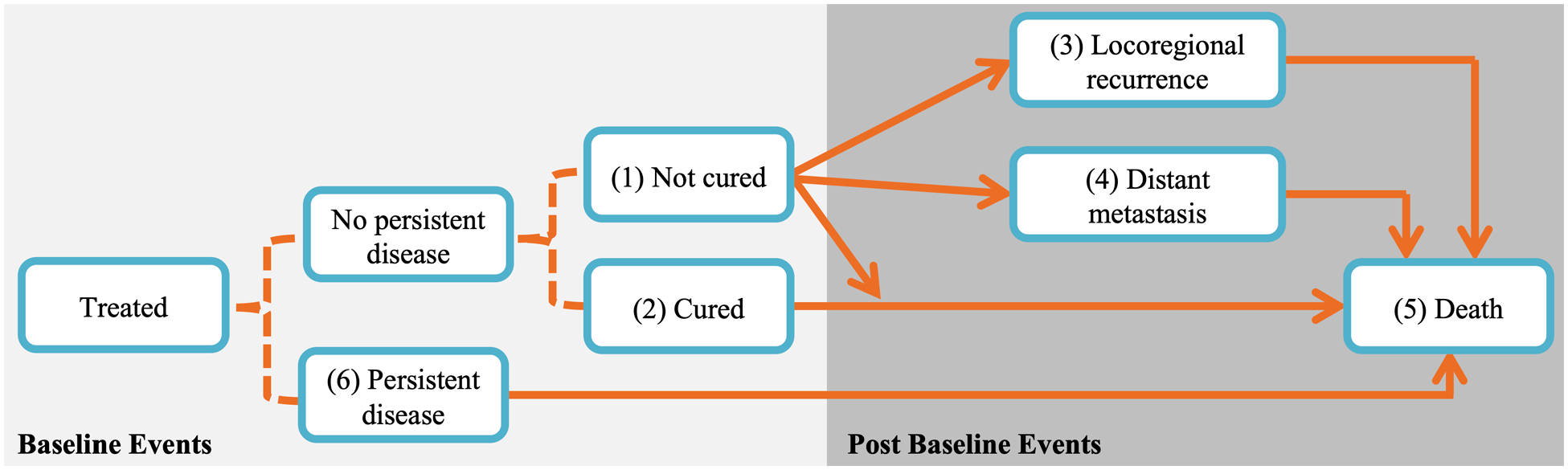For example, the log odds of patient i having persistent disease (as opposed to cured or non-cured disease) is given by $l o g i t (P (G_{i} = 6 | G_{i} \in (1, 2, 6), X_{i})) = γ_{0} + γ X_{i}$ , where $X_{i}$ is a vector of baseline covariates and $G_{i}$ is an indicator for disease state.

Figure 1.

State transition diagram of Bayesian multistate model. Baseline events are modeled using logistic regression (dotted lines) and transitions between post-baseline events are modeled using proportional hazards models (solid arrows). Transitions from states 1 or 2 directly to state 5 correspond to other-cause death, while transitions through state 3, 4, or 6 to state 5 correspond to death after recurrence; these deaths correspond largely to cancer-specific death although death could be due to any cause. Figure is adapted from Beesley et al.²⁰

Patients may subsequently experience a recurrence (either locoregional recurrence or distant metastasis) and/or death. Although patients may experience both types of recurrence, we only consider the type of the first recurrence. The risks of these post-baseline events—locoregional recurrence (state 3), distant metastasis (state 4), and death (state 5)—are modeled using proportional hazards models with Weibull baseline hazard functions. Transitions to locoregional recurrence and distant metastasis assume piecewise baseline hazards with jumps at 6 months. The jump at 6 months was chosen based on empirical patterns seen in the patient data, as explained in Beesley et al.²⁰ For example, the model for subject i’s risk of transitioning from uncured disease (state 1) to locoregional recurrence (state 3) is $λ_{13} (t) = λ_{13}^{0} (t) e^{β_{13} X_{i}}$ where $λ_{13}^{0} (t)$ is the baseline hazard at time $t$ and $e^{β_{13} X_{i}}$ captures the association between the risk of this transition and the vector of baseline covariates, $X_{i}$ . Models for other post-baseline events are similar. Note that for transitions after recurrence, the clock is reset to zero at the time of recurrence. The full details of this MSM are provided in Beesley et al²⁰ but a brief summary—including descriptions of additional component models and order restrictions on some parameters—is presented in the Appendix (Section A.1).

Importantly, the association between patient characteristics and risk of post-baseline events are allowed to differ by event, enabling flexibility to incorporate domain knowledge into the structure of the MSM. Examples include which covariates are included in the models for each state transition and if/how order restrictions are imposed. This structure, along with the MSM’s simultaneous modeling of multiple outcomes, may aid in the accuracy of survival predictions. To account for this complex structure and the large number of parameters required, Bayesian priors are used to impose shrinkage in the MSM. After fitting the MSM using a Markov chain Monte Carlo (MCMC) sampling algorithm, posterior means can be used to calculate state transition probabilities for any set of known covariate values. The model can be used to give predictions of multiple types of events at any follow-up time. Here, we will only consider the outcomes of OS and EFS at two time points (2.5 and 5 years post-diagnosis). Both the models for baseline and post-baseline events capture the magnitude and direction of the association between each covariate and state transition. The MSM also quantifies the uncertainty of these estimates via credible intervals.

Approach to missing data

As described earlier, a substantial proportion of patients in these data have missing covariate values. Within each MCMC iteration, the Substantive Model Compatible Fully Conditional Specification (SMC-FCS) strategy is used to generate single imputations of the missing values.^25,26 This approach, which assumes data are missing at random, involves drawing the missing values from a distribution that incorporates the structure of the MSM and a model for the conditional distribution of each covariate being imputed. For added flexibility, the specific set of covariates included as predictors in each imputation model can differ based on domain knowledge. Auxiliary covariates—including number of sexual partners, HPV DNA presence, and marital status—are also used in the covariate models for imputation. Many of these covariates are particularly useful for imputing missing values of p16, which is an important predictor with a high rate of missingness. Along with missing covariate values, unobserved outcomes (e.g., type of recurrence), and cure status are also imputed within each MCMC iteration. More details, including the full list of auxiliary covariates and imputation models, can be found in Beesley et al.²⁰ Importantly, the description above only applies to handling missing data when building the model. To apply the fitted model to make predictions, we require no missing data in the covariates.

Random survival forest

In contrast to this domain-driven application-specific MSM, the random survival forest (RSF) is a data-driven off-the-shelf approach to modeling event-time outcomes developed by Ishwaran et al.²⁷ The implementation of this data-driven approach is domain-agnostic; however, the method’s non-parametric nature makes it an excellent tool for predictions.

The RSF is a bootstrap-based method in which regression trees are grown on subsets of re-sampled data and then combined back together to produce ensemble estimates. For RSF, the outcome variable for subject i consists of an observed event time $Y_{i}$ and an event indicator $δ_{i}$ , where $Y_{i} = \min (T_{i}, C_{i})$ , $T_{i}$ is the (potentially unobserved) true event time, and $C_{i}$ is the censoring time. In this case study, we consider two event-time outcomes: EFS and OS. We fit a separate RSF for each outcome, in contrast to the MSM which can consider multiple time-to-event outcomes in a single model. Each RSF is made up of many trees (in our case, 1000 trees) fit to bootstrapped versions of the data. Within each tree, patients are iteratively partitioned at nodes based on the covariate value that maximizes the log rank test statistic of survival difference between the daughter nodes. Once terminal nodes reach a pre-specified minimum population size, each terminal node is used to estimate a survival function at time $t$ . These survival estimates are then averaged across the out-of-bag trees; a tree is considered “out-of-bag” for a given observation if that observation was not included in the bootstrapped sample of the data used for original construction of the tree. Using only out-of-bag estimates reduces over-fitting and results in effectively cross-validated estimates of survival probabilities.

Although the RSF can easily be used to estimate survival probabilities like the MSM, unlike the MSM the RSF summarizes covariate effects in less detail using a ranking of the relative importance (called VIMP) of the covariates for a single survival outcome at a time (e.g., only OS or only EFS). The permutation-based VIMP score of a given covariate is calculated as the change in out-of-bag prediction error (measured by concordance; C-index) when the covariate is used as an informative predictor versus permuted.²⁷ While this metric provides information about the relative importance of each covariate, the VIMP score does not directly quantify the magnitude or direction of the association between a covariate and the outcome.

The non-parametric nature of the RSF does not allow for use of parameter restrictions to force clinically-known associations between variables, unlike the MSM, and instead relies exclusively on data to inform associations. We fit RSFs using the R package randomForestSRC. Additional details on this approach can be found in Ishwaran et al and in Ishwaran and Kogalur (2019, 2007).^27-29

Approach to missing data

Within the RSF algorithm, a built-in method imputes missing covariate values. As described above, when a tree is grown on each bootstrapped sample of the data, log-rank tests are used to determine on which variable and at what value to split the data at each node. These log-rank test statistics are calculated using only complete cases. If the candidate variable chosen for the split contains missing values, then these missing covariate values are imputed by drawing randomly from the in-bag (i.e., the present node’s) non-missing values. Patients are then partitioned between daughter nodes using the now-complete data. After the split, filled-in missing values are reset to missing. This imputation mechanism is akin to hot-deck imputation³⁰ and implicitly assumes that data are missing at random.

In contrast to the MSM which uses additional auxiliary variables in the imputation models, the RSF uses only the primary patient characteristics given in Table 1 for imputation and prediction. The role of covariates in the RSF’s imputation process is also not easily interpreted as it accounts for missing data within the black-box estimation procedure. This lack of interpretability contrasts sharply with the imputation approach used by the MSM in which associations between covariates are explicitly specified in parametric models.

While the MSM and RSF each have a variety of advantages and disadvantages, a few primary features distinguish these two approaches; namely, the ability to incorporate domain knowledge and the interpretability of the approach, as well as the ease of implementation. In the following sections, we focus on comparing the predictive accuracy of the MSM and RSF. The above factors, however, are clearly important when choosing the most appropriate approach for a specific objective and have the potential to influence the accuracy of the resulting predictions.

Criteria for evaluation of predictive accuracy

We evaluate the accuracy of estimated survival probabilities at 2.5 and 5 years based on two criteria: discrimination and calibration. The discriminative accuracy of predictions is assessed using area under the receiver operating characteristic curve (AUC) and concordance index (C-index) at each specified time point (2.5 and 5 years). C-index calculations are based on comparing the order of predicted survival probabilities and observed survival times among all possible pairs of observations. Pairs in which the event is not observed for the member with the shorter survival time are excluded from the calculation. These metrics are calculated using the R packages survivalROC³¹ and survival.^32,33 Although AUC and C-index are the same in some settings (e.g., logistic regression³⁴), they are not equivalent in the survival setting due to censoring and thus we consider both AUC and C-index.

The calibration of each approach’s predictions is evaluated by comparing the predicted survival probabilities at 2.5 and 5 years to survival probabilities estimated via Kaplan-Meier (KM) curves. Specifically, patients are placed into 0.10-wide bins based on survival probabilities predicted at a fixed time by the MSM or RSF. The midpoint of each bin is compared to the 2.5- or 5-year survival probability estimated from a KM curve fit to observed data belonging to the patients contained within each bin; the KM estimates represent target calibration. More details on the construction of these calibration plots can be found in the Supplemental Material (Section S1).

For a comprehensive comparison, we analyze the OPSCC data twice. In the first analysis, we fit the models using the entire dataset and evaluate predictions from the same dataset without using any separate test data; we call this the “train-train” approach. In the second analysis, we evaluate predictive accuracy under 10-fold cross validation (CV); we refer to this as the “CV setting” later. The goal of presenting results in the CV setting is to approximate the predictive performance that we would expect on a separate testing dataset (which is not available here).

Both the RSF and MSM account for missing values while being fit, but only the RSF can easily make predictions on a new subset of data containing incomplete cases. The RSF uses an approach similar to the “hot-deck”-like algorithm used during model fitting to make predictions for incomplete cases. The MSM requires complete data to make predictions and so in the CV setting we multiply impute missing values in each left-out subset using multiple imputation via fully conditional specification (MI-FCS) via the mice package in R.³⁵ Imputation models use all original predictors from the MSM (excluding auxiliary covariates), as well as Nelson-Aalen cumulative hazard estimates and event indicators for both death and recurrence, as recommended in White and Royston.³⁶ While MI-FCS is similar to the imputation approach developed as part of the MSM, it does differ slightly and so the imputation approach used on each 9/10ths of the data does not exactly match the approach used on each remaining 1/10th of the data. We make this decision to better match a real-life setting in which an analyst wishes to apply the fitted MSM to a set of new data that contains missing values and only has access to coefficient estimates from the outcome model, thus requiring them to fill in missing values using a separate approach like MI-FCS. This imputation process results in 10 complete versions of each of the left-out datasets, for a total of 100 datasets from which MSM predictions are made. To summarize discriminative accuracy of the predictions, we average the predictions across imputations and then calculate the AUC and C-index for each left-out fold before summarizing cross-validated predictive performance using the average AUC and C-index values. Because multiple imputation is not needed to make predictions using the RSF, we can simply calculate AUC and C-index for each left-out fold and then average the values. We summarize calibration by taking the average of the KM estimates of observed survival within each bin of predicted probabilities across all left-out subsets.

Application to Oropharyngeal Cancer

We fit the MSM and RSF to the OPSCC data using the “train-train” and CV approaches. While the structure of the MSM enables the consideration of multiple time-to-event outcomes in a single model, to facilitate comparison between the MSM and RSF, we fit two RSFs: one for OS and one for EFS. The approaches described previously are used to account for missing data. Additional tuning is required for the RSF; we use out-of-bag C-index as our optimization criterion and find that a terminal node size of 18 subjects and 2 candidate variables, and a terminal node size of 10 and 2 candidate variables, produce the highest C-index for OS and EFS, respectively.

A comparison of predicted survival probabilities—OS and EFS at 2.5 and 5 years—estimated by each approach in the “train-train” setting is shown in Figure 2. Across both event-time outcomes and prediction times, the RSF predicts a narrower range of survival probabilities compared to the MSM. While the MSM predictions span nearly the entire 0 to 1 range of survival probabilities at 5 years, the RSF model predicts no survival probabilities lower than 25%, resulting in substantial disagreement exists at the lower end of the MSM- and RSF-predicted probabilities.

Figure 2.

Comparison of predicted 2.5-year (top row) and 5-year (bottom row) probabilities of overall survival (left column) and event-free survival (right column) from the Bayesian multistate model (MSM) and random survival forest (RSF) in the “train-train” setting. Points with darker outlines correspond to complete cases. The marginal distributions of each set of predictions are shown along each axis.

We also compare the discrimination and the calibration of the predicted survival probabilities estimated by each approach. Table 2 summarizes the discrimination metrics from predictions made using the OPSCC data in the “train-train” setting and under 10-fold CV. Based on AUCs and C-indices of predictions calculated in the “train-train” setting, the MSM outperforms the RSF in terms of discriminative ability. The difference in discriminative ability between the two models narrows in the CV setting, with the accuracy between the two models being quite comparable.

Table 2.

AUCs and C-indices (reported as mean (standard deviation)) for predictions of (A) overall survival and (B) event-free survival at 2.5 and 5 years from the multistate model (MSM) and random survival forest (RSF) fit on the oropharyngeal squamous cell carcinoma data in the “train-train” and cross-validation (CV) settings.

	(A) Overall survival: mean (SD)
	2.5 years				5 years
	AUC		C-index		AUC		C-index
RSF	0.70	-	0.72	-	0.74	-	0.72	-
MSM	0.71	-	0.75	-	0.77	-	0.75	-
CV RSF	0.74	(0.05)	0.73	(0.03)	0.76	(0.03)	0.73	(0.04)
CV MSM	0.74	(0.07)	0.74	(0.04)	0.77	(0.06)	0.74	(0.04)
	(B) Event-free survival: mean (SD)
	2.5 years				5 years
	AUC		C-index		AUC		C-index
RSF	0.70	-	0.69	-	0.72	-	0.69	-
MSM	0.70	-	0.72	-	0.73	-	0.72	-
CV RSF	0.71	(0.03)	0.70	(0.03)	0.73	(0.03)	0.70	(0.03)
CV MSM	0.71	(0.06)	0.71	(0.04)	0.73	(0.06)	0.71	(0.04)

For the CV setting, metrics of discriminative ability are summarized as the mean of all left-out folds. Higher values suggest better performance. Differences of ≥0.02 in AUC or C-index between the RSF and MSM are in bold text.

Abbreviations: AUC, area under the curve; C-index, concordance index; SD, standard deviation.

In Figure 3, we illustrate the calibration of both models’ predictions in the “train-train” setting and under CV at the 2 specified time points. These plots show reasonable calibration from both models. As in Figure 2, these calibration plots reflect the fact that the RSF predicts a narrower range of probabilities than the MSM. Although the RSF-predicted survival probabilities do not span the entire 0 to 1 range, they do appear to be well calibrated to the KM-estimated survival probabilities. The MSM does predict the full range of survival probabilities but shows deteriorating calibration for low probabilities of survival. The 95% confidence intervals for the KM estimates are wider for the predictions in the CV setting than for predictions in the “train-train” setting because predictions are made on datasets 1/10th the size of the original data.

Figure 3.

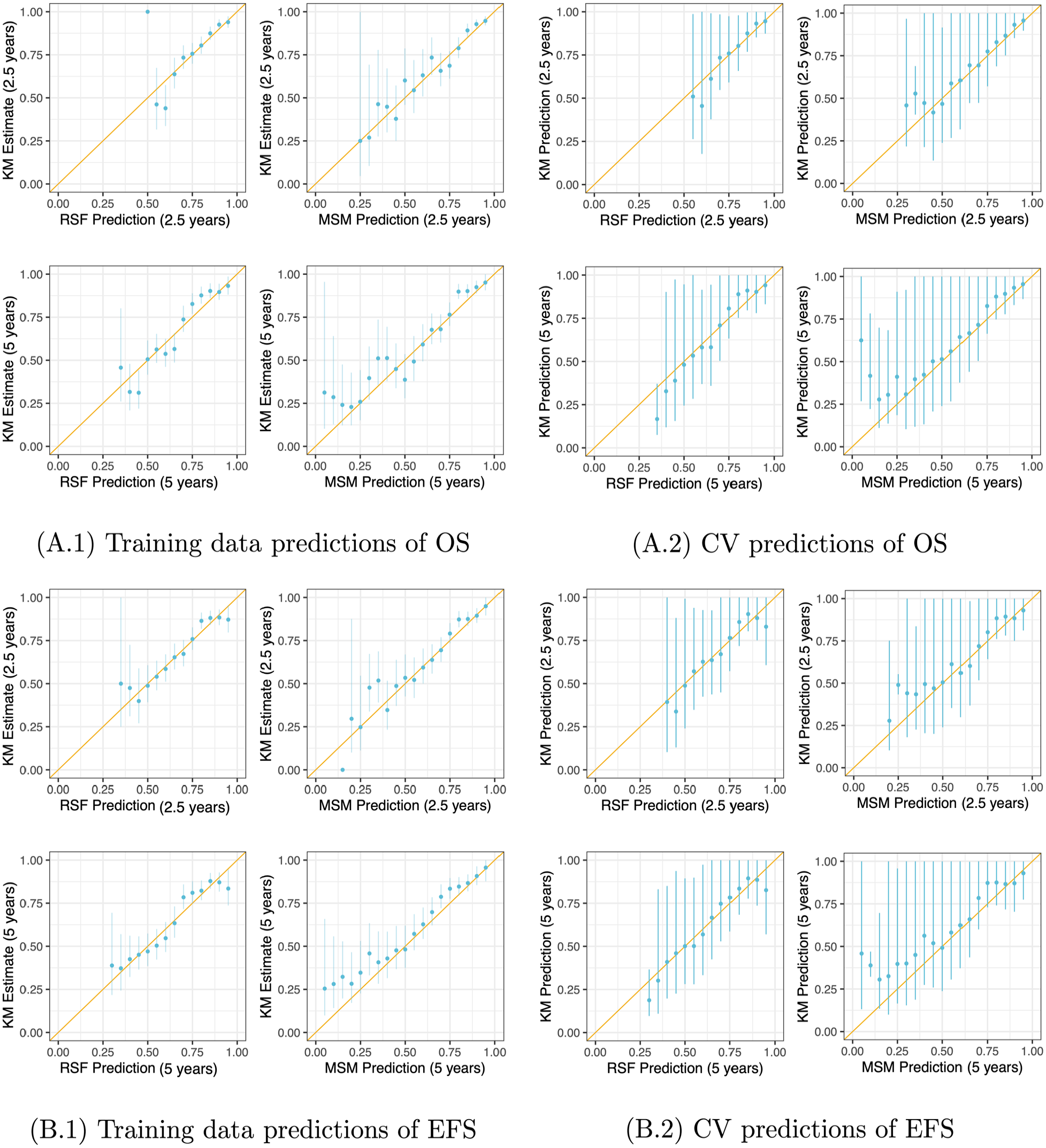
Calibration of (A) overall survival (OS) and (B) event-free survival (EFS) predictions at 2.5 and 5 years from the multistate model (MSM) and random survival forest (RSF) fit using the oropharyngeal squamous cell carcinoma data in the “train-train” setting (A.1, B.1) and using 10-fold cross-validation (CV) (A.2, B.2). In the CV setting, predictions were estimated on all left-out folds and then used to place observations in the testing data into bins; Kaplan-Meier (KM) survival curves were estimated using testing data in each bin. These KM estimates and model-based predictions were then pooled and plotted here. The diagonal yellow line indicates perfect calibration. The vertical blue lines denote 95% confidence intervals for the KM estimates of survival probability based on pooled variance estimates.

While the MSM provides coefficient estimates and credible intervals (see Figure A1 in the Appendix), variable importance (VIMP) is commonly used with RSFs as an alternative method for assessing the “importance” of each covariate in the RSF algorithm. For each RSF (for the outcomes of OS and EFS), VIMP scores are plotted in Figure A2 in the Appendix. We find that that coefficient estimates from the MSM match clinical intuition (e.g., negative p16 status is strongly associated with increased risk of locoregional recurrence, death after locoregional recurrence, and persistent disease), but that missingness rates can drive the VIMP scores for covariates in the RSF. For example, when VIMP scores are calculated from RSFs fit to all available data, p16 status has a relatively low VIMP score (6th out of 8 predictors for both OS and EFS). When the RSF is refit to complete cases only, the VIMP score for p16 increases, resulting in this covariate ranking fourth and third for the outcomes of OS and EFS, respectively. Similar trends are seen among other covariates with missing data; further discussion is provided in the Appendix (Section A.3). Overall, it is important to note that the rate of missingness does appear to influence VIMP scores in an undesirable manner.

Simulation Study

In the results presented in the previous section, we were surprised that after cross-validation the predictive accuracy of the off-the-shelf RSF was comparable to that of the highly specialized MSM, despite the difference in the complexity of their missing data approaches and in the amount of domain-specific knowledge incorporated into their structures. In this section, we aim to gain a better understanding of how robust the RSF’s data-driven non-parametric approach—to both imputation and outcome modeling—is to various amounts and types of missing data, relative to a parametric approach to analysis. Additionally, we investigate whether the structural/disease progression information that is part of the MSM gives any advantage over the RSF’s approach that ignores this structure.

Examining imputation approaches for handling missing data

We conduct simulations to better understand the robustness of the RSF’s hot deck approach³⁰ for imputation compared to a parametric approach—multiple imputation by fully conditional specification (MI-FCS) with a Weibull regression outcome model—within a simpler survival analysis setting of a single event time with various patterns and amounts of missing data. MI-FCS is implemented using the mice package.³⁵

Data generation: We generate a training dataset and a testing dataset, each with a sample size of N = 1000. Both datasets consist of six covariates generated from a standard normal distribution, two pairs of which are correlated and two of which are independent. We generate a true survival time from an exponential distribution with the mean as a function of covariate main effects and interactions and generate a censoring time from an exponential distribution with constant mean. For half of the predictors, we induce missingness at three different within-variable levels (25%, 50%, and 75%) under two different mechanisms: (i) missing completely at random (MCAR) and (ii) missing at random (MAR). Additional details describing this data generation and missingness process are given in the Appendix (Section A.4.1). Testing data are simulated using the same process as outlined above, but no missingness is induced.

In modeling of the survival outcome, we account for the missing values in two different ways: when using the fully parametric analysis approach (Weibull regression), we multiply impute (M = 10) the missing values using MI-FCS, with all six covariates as predictors (main effects only) along with the Nelson-Aalen estimate of the cumulative hazard (evaluated at the observed event time) and the event indicator.³⁶ When using the fully non-parametric analysis approach, we rely on the RSF’s built-in imputation algorithm. We also consider a third intermediate analysis approach that combines the parametric approach to imputation (MI-FCS) and the non-parametric approach to modeling the outcome (RSF).

We then apply each analysis approach—the fully parametric approach that uses MI-FCS for imputation and models the outcome using a Weibull regression model with main effects only, the fully non-parametric approach that uses the RSF for both imputation and outcome modeling, and the intermediate approach that combines MI-FSC and the RSF—to each training dataset with a different pattern of missingness. We estimate survival probabilities at 2.5 years for the training and testing data and evaluate discrimination and calibration of predictions. For the Weibull models fit to the imputed datasets, we average the coefficients across the multiple datasets prior to making predictions. As the RSF does not return coefficient estimates, when applying this approach to the imputed datasets we instead average predictions across the 10 imputed datasets prior to evaluating performance. For RSF predictions on the training data, we only consider out-of-bag predictions. (Note that the concept of “out-of-bag” does not apply to the testing data.) Performance is summarized as average AUC and C-index. We also calculate predictions from the Weibull regression model used to generate the data (with true parameter values and interaction terms), as well as a Weibull regression model with main effects only and a RSF both fit to the complete data; we use the predictive performance of these 3 models as benchmarks in our evaluation. We repeat this process of data generation, estimation, prediction, and performance evaluation 100 times.

Results: We focus first on comparing the fully parametric approach to analysis (i.e., Weibull regression with imputation via MI-FCS) with the fully non-parametric approach to analysis (i.e., RSF for imputation and outcome modeling). The fully parametric approach generally outperforms the fully non-parametric approach in terms of discriminative accuracy across all missing data mechanisms in the testing data, as indicated by larger testing AUCs and C-indices (see Table 3A), except when little data are missing. As the amount of missingness increases, the performance of the RSF deteriorates faster than that of the Weibull regression model.

Table 3.

Results from simulation studies examining (A) imputation approaches and (B) structural components.

(A) Discriminative accuracy in simulation study examining imputation approaches
			Training				Testing
Missingness	Imp. Model	Outcome model	AUC (SD)		C-index (SD)		AUC (SD)		C-index (SD)
None	None	Data-generating	0.74	(0.02)	0.70	(0.01)	0.74	(0.01)	0.71	(0.01)
None	None	Weibull	0.73	(0.02)	0.69	(0.01)	0.72	(0.02)	0.69	(0.01)
None	None	RSF	0.72	(0.02)	0.69	(0.01)	0.73	(0.02)	0.69	(0.01)
MCAR 25%	MI-FCS	Weibull	0.72	(0.02)	0.69	(0.01)	0.71	(0.02)	0.69	(0.01)
MCAR 25%	MI-FCS	RSF	0.72	(0.02)	0.69	(0.02)	0.72	(0.02)	0.69	(0.01)
MCAR 25%	RSF	RSF	0.68	(0.02)	0.66	(0.01)	0.71	(0.02)	0.68	(0.01)
MCAR 50%	MI-FCS	Weibull	0.71	(0.02)	0.69	(0.01)	0.71	(0.02)	0.68	(0.01)
MCAR 50%	MI-FCS	RSF	0.74	(0.02)	0.70	(0.02)	0.71	(0.02)	0.68	(0.01)
MCAR 50%	RSF	RSF	0.65	(0.02)	0.64	(0.01)	0.69	(0.02)	0.67	(0.01)
MCAR 75%	MI-FCS	Weibull	0.71	(0.02)	0.68	(0.01)	0.70	(0.02)	0.68	(0.01)
MCAR 75%	MI-FCS	RSF	0.75	(0.03)	0.72	(0.02)	0.71	(0.02)	0.68	(0.01)
MCAR 75%	RSF	RSF	0.63	(0.02)	0.61	(0.01)	0.67	(0.02)	0.64	(0.01)
MAR 25%	MI-FCS	Weibull	0.72	(0.02)	0.69	(0.01)	0.71	(0.02)	0.69	(0.01)
MAR 25%	MI-FCS	RSF	0.73	(0.02)	0.69	(0.02)	0.72	(0.02)	0.69	(0.01)
MAR 25%	RSF	RSF	0.68	(0.02)	0.66	(0.01)	0.71	(0.02)	0.68	(0.01)
MAR 50%	MI-FCS	Weibull	0.71	(0.02)	0.69	(0.01)	0.71	(0.02)	0.68	(0.01)
MAR 50%	MI-FCS	RSF	0.75	(0.03)	0.71	(0.02)	0.71	(0.02)	0.68	(0.01)
MAR 50%	RSF	RSF	0.65	(0.02)	0.64	(0.01)	0.69	(0.02)	0.66	(0.01)
MAR 75%	MI-FCS	Weibull	0.71	(0.02)	0.68	(0.01)	0.70	(0.02)	0.68	(0.01)
MAR 75%	MI-FCS	RSF	0.77	(0.04)	0.73	(0.03)	0.70	(0.02)	0.67	(0.01)
MAR 75%	RSF	RSF	0.62	(0.02)	0.61	(0.01)	0.65	(0.02)	0.64	(0.01)
(B) Discriminative accuracy in simulation study examining structural components
		Mean AUC (SD)					Mean C-index (SD)
Time	Outcome	MSM	RSF				MSM		RSF
0.5	OS	0.70 (0.02)	0.71 (0.02)				0.70 (0.01)		0.68 (0.01)
1	OS	0.75 (0.02)	0.74 (0.02)				0.70 (0.01)		0.69 (0.01)
0.5	EFS	0.66 (0.02)	0.66 (0.02)				0.64 (0.01)		0.63 (0.01)
1	EFS	0.72 (0.02)	0.70 (0.02)				0.64 (0.01)		0.63 (0.01)

In (A), we consider a single event outcome and summarize discriminative performance under various missingness mechanisms and amounts; “data-generating” refers to predictions from the true model used to simulate the data, which includes interaction terms. In (B), we consider two event outcomes (recurrence and death), which are modeled with a single illness-death multistate model (MSM) and two random survival forests (RSFs)—one for overall survival (OS) and one for event-free survival (EFS). Test set discriminative performance of the MSM and RSFs for predictions of OS and EFS at 0.5 and 1 year are shown. Bold text denotes differences ≥0.02 in area under the curve (AUC) or concordance index (C-index) between analysis approaches within comparable scenarios.

Abbreviations: MAR, missing at random; MCAR, missing completely at random; SD, standard deviation.

We then compare the discriminative accuracy across the parametric and non-parametric outcome models when both are fit using training data imputed with parametric MI-FCS. We find that the discriminative accuracy of predictions from the RSF fit to data imputed using MI-FCS is generally higher than that from the Weibull regression model fit to data also imputed using MI-FCS when missingness is moderate to high. However, although we always evaluate the RSF’s predictive performance on the training data using out-of-bag predictions, we find that AUC and C-index values from training data predictions made using the combined MI-FCS + RSF approach do not closely match those from the testing data. Instead, the training AUC and C-index values appear to be inflated. This over-optimism in performance exists even though out-of-bag predictions attempt to mimic predictions from a separate validation dataset. Furthermore, this inflation of discriminative performance contrasts with the conservative nature of the AUC and C-index values from training data predictions made using only the RSF for both imputation and outcome modeling; in this setting, using out-of-bag predictions results in AUC and C-index values that are overcorrected and underestimate the true discriminative performance on testing data.

Among the calibration plots (in Figure A3 for testing data only), the plot labeled “Data-generating” corresponds to predictions calculated using the true coefficient values and true interaction terms in a Weibull model; we interpret this plot as showing ideal calibration when no estimation error or model misspecification is present. The plot labeled “Weibull: complete” illustrates the calibration of predictions made from a Weibull regression model fit to the complete data; this plot tells us what sort of calibration we can hope for in a more realistic setting in which the true associations (i.e., interactions) between the predictors and outcome are unknown but no error due to missing data is present. Similarly, the plot labeled “RSF: complete” corresponds to realistic target calibration of predictions from the RSF without error due to missing data. We notice that if the true interactions between covariates are unknown in this Weibull regression model, realistically we cannot achieve perfect calibration: in the plot labeled “Weibull: complete,” the upper tail of predicted probabilities overestimates true survival. Thus, we attribute this deterioration in calibration seen for the other Weibull models to the lack of interaction effects, rather than the presence of missing data.

The predictions from both the RSF and Weibull models in the presence of missing data show similar calibration accuracy, regardless of whether a parametric or non-parametric imputation approach is used for the RSF. The slightly S-shaped calibration curves for the RSF indicate that it tends to predict more moderate survival probabilities.

We conduct additional simulations comparing the performance of the RSF and parametric Weibull model in similar settings but with (i) additional non-informative predictors and (ii) auxiliary variables for imputation. Overall, we find patterns in performance similar to those found here. Results from these simulations are presented in more detail in the Supplemental Material (Section S4).

Examining structural components

The goal of the second simulation is to evaluate the potential benefit conferred to the MSM by its structural components, compared to the RSF. In this context, we use the phrase “structural components” to refer to the multiple states and transitions between states that are explicitly specified within the model. The MSM considered here is a simple illness-death model that consists of three states—treatment, recurrence, and death—and three possible transitions: treatment to recurrence, treatment directly to death, or death following recurrence. Although the baseline hazards of this illness-death model are assumed to be non-parametric, we believe that comparing this illness-death model to RSFs (which can each only evaluate a single time-to-event outcome at once due to their lack of structure) allows us to evaluate the contribution of the additional structure to the illness-death model’s predictive accuracy.

Data generation: We simulate transition times for 1000 subjects using three different Weibull distributions, with the scale parameter a function of covariate values and the coefficients on each covariate varying by transition. For more details, see the Appendix (Section A.5.1). We then fit the illness-death model using the mstate package.^37-39 We use the “clock-reset” approach with transition-specific covariate effects and no restriction on proportionality of baseline hazards between transitions. We only include main effects and no interactions in both data generation and model fitting, and do not induce missingness. Two RSFs (one for OS and one for EFS) are fit using the randomForestSRC package with default tuning parameter values.^27-29

Next, we generate new data for validation. We compare the discrimination and calibration of survival predictions for two outcomes—OS and EFS at 0.5 and 1 year—for the 1000 patients contained in these testing data. We repeat data generation, estimation, prediction, and performance assessment 100 times and summarize the predictive performance on the testing data across all 100 repetitions.

We also evaluate the predictive performance of two Cox proportional hazards models—one for OS and one for EFS—in an attempt to compare the performance of the illness-death model to an alternative parametric model that lacks structural information. We present the results of this additional simulation study in the Supplemental Material (Section S5.3).

Results: The discriminative performance, summarized as the mean (standard deviation) of AUC and C-index, is reported in Table 3B. We see that the RSF and the illness-death model perform similarly in terms of discriminative accuracy. The discriminative accuracy of the illness-death model improves slightly relative to that of the RSF at later time points. Overall neither the RSF nor illness-death model consistently outperforms the other by a large margin when predicting OS or EFS. However, the AUC and C-index for the MSM are often very slightly larger than those of the RSF.

We plot the calibration of predictions in Supplemental Figure S7. We find that the predictions from the illness-death model and the RSF are similarly well-calibrated in the range of mid-to-high survival probabilities. The illness-death model shows slightly more stable calibration than the RSF and, when considering the probability of OS at 0.5 year, we also see that the RSF predicts a narrower range of survival probabilities than the illness-death model. For the outcome of EFS, both the illness-death model and RSF tend to slightly overestimate high probabilities of survival compared to the KM estimates.

As an alternative check of the calibration of these predictions, we also compare the predicted probabilities of OS and EFS to true survival probabilities for each subject by calculating true survival probabilities using KM curves estimated from a larger simulated dataset (see Section S2 for details). In Figure 4, we compare the true KM-based survival probabilities to the model-based predicted probabilities for all patients (N = 1000) in the testing data in a single iteration of this simulation. We see that there is less variability around the truth in the illness-death model’s predictions of survival than for the RSF. We also see that the illness-death-predicted probabilities span a greater range than the RSF-predicted probabilities, reinforcing what we previously noted: the data-driven non-parametric approach (the RSF) tends to predict more moderate survival probabilities while the domain-driven parametric and semi-parametric models (illness-death model, Weibull regression, and Bayesian MSM) predict a larger range of probabilities.

Figure 4.

Results from a single iteration of the simulation comparing structural components. Comparison of RSF- and illness-death MSM-predicted probabilities to simulated “true” survival probabilities for all subjects in a single testing dataset. Smooth curves show trends in predictions from each approach using generalized additive models. Ideally, points would fall along the diagonal. For more details on calculation of true survival curves, see the Supplemental Material (Section S2).

We conduct additional variations of this simulation study to determine if different sample sizes or transition and censoring rates impact the predictive performance of the illness-death model or the RSF. We find that reducing the sample size by 50% or increasing it by 100% does not substantially impact predictive performance; we also find that when the rate of observed events is lower, the illness-death model may have a slight advantage over the RSF, although the difference in predictive performance is very slight. Details on these additional simulations and their results are given in the Supplemental Material (Sections S5.1 and S5.2).

Discussion

We found that the domain-driven Bayesian MSM and the data-driven RSF had similar predictive accuracy when applied to the OPSCC data, despite the MSM’s more complex structure and domain-driven approach to imputation. Though the predictive accuracy was overall similar, in many instances the MSM very slightly outperformed the RSF. Through this illustrative example with clinical data supplemented with simulations, we saw that the RSF tended to predict a narrower range of survival probabilities than the parametric models. When predictions were calculated for patients contained in the OPSCC data, substantial disagreement between the MSM- and RSF-predicted probabilities existed for lower estimates of survival. If these two approaches were to be applied in a clinical setting, the choice of statistical approach would have the potential to substantially impact predictions of prognosis for some patients.

Our simulation results suggest that when predictors have high rates of missingness, as seen for some clinical covariates in the OPSCC data, the performance of the RSF’s built-in non-parametric method for imputation can deteriorate. Our simulation results also indicate that combining a parametric approach to imputation—MI-FCS—with a non-parametric approach for outcome modeling—RSF—has the potential to result in accurate predictions in the presence of substantial missingness. Based on these simulation results, we re-analyze the OPSCC data by applying the RSF to data multiply imputed using MI-FCS (see Table A4 for results). We find that when MI-FCS is combined with the RSF, the discriminative accuracy of predictions in the “train-train” setting are higher than that of the domain-driven MSM and the fully non-parametric RSF (i.e., when the RSF is used for both imputation and outcome modeling); however, from simulation results we know that these estimates of predictive accuracy are likely overly optimistic. In the CV setting, this difference decreases and the discriminative accuracy of predictions from all approaches are quite comparable, suggesting that perhaps rates of missing data are low enough for the RSF’s built-in imputation approach to perform satisfactorily in this application.

The treatments the patient received are not considered as covariates in this work. There is variation in the treatments they received, but it generally follows treatment guidelines, which are highly influenced by T and N stage of disease. Because of this high level of confounding, we did not include treatments as variables in the MSM and RSFs.

Calibration plots suggested that probabilities predicted by the RSF are well calibrated, despite being concentrated at moderate values. The tendency of the RSF to predict a narrower range of survival probabilities could be related to the non-parametric data-driven nature of the RSF: this approach is less likely to extrapolate covariate effects and predict extreme survival probabilities than the domain-driven parametric and semi-parametric models. We also noted that assessments of predictive accuracy made using the RSF’s out-of-bag predictions for training data (when the RSF’s built-in approach is also used for imputation) tend to underestimate the approach’s performance on a new testing dataset. We attribute this conservative assessment of performance to the internal cross-validation/regularization built into the RSF algorithm via bootstrapping and out-of-bag predictions, as supported by inflated AUC and C-index values when out-of-bag predictions are not used (see Table A5 in the Appendix). However, when MI-FCS is combined with the RSF, out-of-bag predictions overestimate the true (i.e., testing data) discriminative accuracy. This suggests that MI-FCS could be contributing to overfitting in this setting. These results emphasize the importance of using a separate testing dataset to evaluate predictive performance, as we have shown various scenarios in which out-of-bag predictions from the RSF do not give accurate estimates of the true predictive performance.

In our simulation study comparing parametric and non-parametric imputation approaches, we saw that when there is little missing data, the predictive accuracy of the RSF and the parametric model were similar. However, the RSF’s imputation approach was less robust against large amounts of missing data than the parametric approach. In the calibration plots, we saw that if the true interactions between covariates were unknown and thus not specified in the Weibull regression model, we realistically could not achieve perfect calibration. This underscored a well-known advantage of the RSF: regression trees are well suited for modeling data involving complex interactions.

Ability to incorporate domain knowledge: When considering the clinical utility of these prediction models, other information provided by a model (e.g., measures of association) should also be considered. Here, the MSM has the advantage of providing estimates of intermediate probabilities—the probability of occupying a specific state at a given time—in addition to probabilities of OS and EFS. The RSF, however, is limited to considering each event-time outcome independently. In both the clinical data application and in our simulation study evaluating the advantage conferred by the structural components of the MSM, we saw that the additional structure of the Bayesian MSM and simple illness-death model provided a very slight advantage over the RSF in terms of discriminative accuracy. In our illness-death model simulation, we also saw less variability in the predicted survival probabilities around the truth. Overall, the advantage of the parametric models over the non-parametric RSF was surprisingly small, however, given the additional information being used in these parametric models.

Another advantage of the parametric approach to prediction stems from the ability to specify biologically-informed monotone associations between patient characteristics and survival probabilities. For example, because a positive monotone association between age and risk of death is explicitly specified in the MSM, the survival probability for a given patient with a fixed set of covariates will not increase as the patient ages. Predicted survival probabilities from the RSF, on the other hand, are not guaranteed to decrease monotonically as age increases, resulting in survival predictions with potentially less clinical relevance. We illustrate this pattern by plotting RSF and MSM predictions of OS and EFS for sets of fixed characteristics but with varying age in the Supplemental Material (Section S3). Although the MSM predictions are smooth, linear effects in the MSM may lead to poor extrapolation near the edges of covariate domains.

These conclusions, however, are based only on our specific MSM (i.e., our choice to include main effects only in the model) and our specific simulation and data generation process (i.e., our choice to include certain interaction terms). The performance of the MSM could be enhanced by the addition of interaction terms, non-linear terms, or transformations, among other modifications. In a real data analysis, exploring these options in the context of the given data and application would be key to selecting an appropriate and well-fitting model.

Interpretability: The MSM also has the advantage of quantifying the associations between clinical characteristics and event-time outcomes (in particular, multiple related event-time outcomes simultaneously) through posterior mean estimates and credible intervals. Results of the MSM show that higher N stage is positively associated with decreased probability that treatment will cure the disease and increased risk of distant metastasis. The RSF, however, only provides relative rankings of variable importance based on VIMP, a measure that neither has a clear interpretation nor provides information on the magnitude or direction of the association between a covariate and an outcome. Numerous alternative approaches to “post-hoc interpretation,” as termed in Pintelas et al,⁴⁰ do exist (e.g., SHapley Additive exPlanations (SHAP)⁴¹ and local interpretable model-agnostic explanations (LIME)⁴) and can provide additional information beyond simply rankings of variable importance. However, these approaches do require using a separate method to interpret predictions on top of an already-fitted black box model.

Furthermore, when a substantial proportion of values are missing in a dataset, VIMP may not provide an accurate representation of the relative importance of the covariates in the population; rather, VIMP only reflects the relative importance of observed covariates within the specific sample and does not necessarily allow generalizable conclusions to be drawn. When comparing the VIMP score for p16—a predictor with biologically-confirmed importance—from the RSF fit on all data versus complete cases, we saw that the ranking of p16 increased when only complete cases were considered. Based on these results, we hypothesized that VIMP scores for predictors with larger amounts of missing data would be biased downward. Through simulations, we confirmed that predictors with larger amounts of missing data tended to have larger VIMP scores in RSFs fit to complete data compared to RSFs fit to all data. This example illustrates that while the RSF does provide some measure of variable importance, these VIMP scores can be misleading and frequently underestimate the true variable importance within the population, particularly when substantial missingness exists in the sample.

If these statistical approaches were to be applied in a clinical setting, the interpretability of the MSM could provide it with an advantage over the RSF. In the MSM, the role of each covariate in each transition is apparent, along with the influence of each covariate on predicted survival probabilities; a similar level of understanding cannot be extracted from the RSF. Presenting measures of association between patient characteristics and the outcome in conjunction with predicted probabilities would improve understanding of the main factors driving the prediction and could increase confidence in the reliability of a calculator’s predictions if used in a clinical setting. Estimates of uncertainty of these associations also emphasize the corresponding uncertainty of the calculator’s predictions.

Ease of implementation: The RSF may provide less information about associations present in the data than the MSM, but it does have a computational advantage. The code for the MSM took many months to develop and the program takes over 5 hours to fit, but the RSF takes only a few minutes. This difference in computational cost influences the ease of evaluating the performance of each model via cross-validation.

Conclusions

Through a case study of prognostic predictions for patients with OPSCC, we found that the domain-driven MSM shows a slight predictive advantage over the black-box RSF, despite substantial differences in the level of biological information incorporated into these two approaches. Data-driven machine learning methods, like the RSF, are designed specifically for the problem of prediction and so they tend to excel at this task. Parametric models are often designed for understanding associations and modeling structural aspects of the data but are less frequently optimized for prediction. However, when rates of missingness are high, we found that the parametric structure provided some advantage over data-driven nonparametric approaches. Results from this case study and from simulation studies suggest that, in addition to predictive accuracy, consideration of other differences (e.g., interpretability) are key when selecting the best statistical approach for addressing the research question at hand. Ultimately, selecting the approach that has the greatest potential to aid in clinical treatment decisions requires thoughtful consideration of the specific goals.

Supplemental Material

sj-docx-1-cix-10.1177_11769351231183847 – Supplemental material for Comparing Individualized Survival Predictions From Random Survival Forests and Multistate Models in the Presence of Missing Data: A Case Study of Patients With Oropharyngeal Cancer

Supplemental material, sj-docx-1-cix-10.1177_11769351231183847 for Comparing Individualized Survival Predictions From Random Survival Forests and Multistate Models in the Presence of Missing Data: A Case Study of Patients With Oropharyngeal Cancer by Madeline R Abbott, Lauren J Beesley, Emily L Bellile, Andrew G Shuman, Laura S Rozek and Jeremy M G Taylor in Cancer Informatics

Supplemental Material

sj-docx-2-cix-10.1177_11769351231183847 – Supplemental material for Comparing Individualized Survival Predictions From Random Survival Forests and Multistate Models in the Presence of Missing Data: A Case Study of Patients With Oropharyngeal Cancer

Supplemental material, sj-docx-2-cix-10.1177_11769351231183847 for Comparing Individualized Survival Predictions From Random Survival Forests and Multistate Models in the Presence of Missing Data: A Case Study of Patients With Oropharyngeal Cancer by Madeline R Abbott, Lauren J Beesley, Emily L Bellile, Andrew G Shuman, Laura S Rozek and Jeremy M G Taylor in Cancer Informatics

Footnotes

Acknowledgements

The authors gratefully acknowledge the contributions of the investigators in the University of Michigan HNSPORE/HNOP for their work in patient recruitment and data collection. We thank Carol R. Bradford, MD, Thomas E. Carey, PhD, Douglas B. Chepeha, MD, Sonia Duffy, PhD, Avraham Eisbruch, MD, Joseph Helman, DDS, Kelly M. Malloy, MD, Jonathan McHugh, MD, Scott A. McLean, MD, Tamara H. Miller, RN, Jeff Moyer, MD, Mark E. Prince, MD, Nancy Rogers, RN, Matthew E. Spector, MD, Nancy E. Wallace, RN, Heather Walline, PhD, Brent Ward, DDS, Francis Worden, MD and Gregory T. Wolf, MD. We are also grateful to patients and their families for their willingness to participate in survey and specimen collections in the University of Michigan HNSPORE/HNOP.

Funding:

The author(s) disclosed receipt of the following financial support for the research, authorship, and/or publication of this article: This research was partially funded by NIH grants CA-129102 and CA-97248 and CA-83654. LJB was partially funded by the LDRD Richard Feynman Postdoctoral Fellowship 20210761PRD1. This work is approved for distribution under LA-UR-22-24202. The findings and conclusions in this report are those of the authors and do not necessarily represent the official position of Los Alamos National Laboratory. Los Alamos National Laboratory, an affirmative action/equal opportunity employer, is managed by Triad National Security, LLC, for the National Nuclear Security Administration of the U.S. Department of Energy under contract 89233218CNA000001.

Declaration Of Conflicting Interests:

The author(s) declared no potential conflicts of interest with respect to the research, authorship, and/or publication of this article.

Author Contributions

MRA: data curation, data analysis, design of simulation study, interpretation of results, visualization, drafting of original manuscript, revision of manuscript. LJB: data curation, methodology, data analysis, design of simulation study, interpretation of results, revision of manuscript. ELB, AGS, LSR: data curation, revision of manuscript. JMGT: methodology, design of simulation study, interpretation of results, funding acquisition, supervision, drafting of original manuscript, revision of manuscript. All authors read and approved the final manuscript.

Availability of Data

Patient data are not publicly available due to privacy restrictions.

Research Ethics and Patient Consent

This work consists of secondary analyses of de-identified patient data. Collection and analyses of the data were done in accordance with relevant guidelines and regulations. Patient data collection was approved by the institutional review board of the University of Michigan. Informed written consent was provided by all patients and there was no financial compensation.

ORCID iD

Madeline R Abbott

Supplemental Material

The appendix and supplemental material for this article are available online.

References

Hippisley-Cox

Coupland

Development and validation of risk prediction algorithms to estimate future risk of common cancers in men and women: prospective cohort study. BMJ Open. 2015;5:e007825.

Beesley

Morgan

Spratt

, et al. Individual and population comparisons of surgery and radiotherapy outcomes in prostate cancer using Bayesian multistate models. JAMA Netw Open. 2019;2:e187765.

Aminian

Zajichek

Arterburn

, et al. Predicting 10-year risk of end-organ complications of type 2 diabetes with and without metabolic surgery: A machine learning approach. Diabetes Care. 2020;43:852-859.

Ribeiro

Singh

Guestrin

. “Why should I trust you?”: Explaining the predictions of any classifier. Proc Annu Conf, Assoc Comput Mach, 22nd. 2016:1135-1144.

Lefèvre

Sun

Bajcsy

, et al. Comparison of parametric and non-parametric approaches for vehicle speed prediction. 2014 American Control Conference, 2014:3494-3499. doi: 10.1109/ACC.2014.6858871.

Ying

Heitjan

Chen

TT.

Nonparametric prediction of event times in randomized clinical trials. Clin Trials. 2004;1:352-361.

Zhao

Yan

Van Hentenryck

Prediction and behavioral analysis of travel mode choice: A comparison of machine learning and logit models. Travel Behav Soc. 2020;20:22-35.

Parmezan

ARS

Souza

VMA

Batista

GEAPA

. Evaluation of statistical and machine learning models for time series prediction: identifying the state-of-the-art and the best conditions for the use of each model. Inf Sci. 2019;484:302-337.

González-Recio

Rosa

GJM

Gianola

Machine learning methods and predictive ability metrics for genome-wide prediction of complex traits. Livest Sci. 2014;166:217-231.

10.

Steingrimsson

JA.

Personalized risk prediction in clinical oncology research: applications and practical issues using survival trees and random forests. J Biopharm Stat. 2018;28:333-349.

11.

Bonneville

Resche-Rigon

Schetelig

Putter

de Wreede

LC.

Multiple imputation for cause-specific Cox models: assessing methods for estimation and prediction. Stat Methods Med Res. 2022;31:1860-1880.

12.

Clark

Ostrander

Cushing

BM.

A multistate model predicting mortality, length of stay, and readmission for surgical patients. Health Serv Res. 2016;51:1074-1094.

13.

Jackson

Tom

Kirwan

, et al. A comparison of two frameworks for multi-state modelling, applied to outcomes after hospital admissions with COVID-19. Stat Methods Med Res. 2022;31:1656-1674.

14.

Pan

Kavanagh

Stewart

, et al. Comparison of multistate model, survival regression, and matched case-control methods for estimating excess length of stay due to healthcare-associated infections. J Hosp Infect. 2022;126:44-51.

15.

Eleuteri

Taktak

AFG

Coupland

Heimann

Kalirai

Damato

Prognostication of metastatic death in uveal melanoma patients: A Markov multi-state model. Comput Biol Med. 2018;102:151-156.

16.

Janssen

Donders

Harrell

Jr , et al. Missing covariate data in medical research: To impute is better than to ignore. J Clin Epidemiol. 2010;63:721-727.

17.

Jerez

Molina

García-Laencina

, et al. Missing data imputation using statistical and machine learning methods in a real breast cancer problem. Artif Intell Med. 2010;50:105-115.

18.

Bertsimas

Pawlowski

Zhuo

YD.

From predictive methods to missing data imputation: an optimization approach. J Mach Learn Res. 2018; 18:1-39.

19.

Perez-Lebel

Varoquaux

Le Morvan

Josse

Poline

JB.

Benchmarking missing-values approaches for predictive models on health databases. GigaScience. 2022;11:1-22.

20.

Beesley

Shuman

Mierzwa

, et al. Development and assessment of a model for predicting individualized outcomes in patients with oropharyngeal cancer. JAMA Netw Open. 2021;4:e2120055.

21.

Beesley

Hawkins

Amlani

, et al. Individualized survival prediction for patients with oropharyngeal cancer in the human papillomavirus era. Cancer. 2019;125:68-78.

22.

Hawkins

Mierzwa

Bellile

, et al. Impact of American Joint Committee on Cancer Eighth Edition clinical stage and smoking history on oncologic outcomes in human papillomavirus-associated oropharyngeal squamous cell carcinoma. Head Neck. 2019;41:857-864.

23.

Peterson

Bellile

Wolf

, et al. Cigarette use, comorbidities, and prognosis in a prospective head and neck squamous cell carcinoma population. Head Neck. 2016;38:1810-1820.

24.

Duffy

Taylor

Terrell

, et al. Interleukin-6 predicts recurrence and survival among head and neck cancer patients. Cancer. 2008;113:750-757.

25.

Beesley

Bartlett

Wolf

Taylor

JM.

Multiple imputation of missing covariates for the Cox proportional hazards cure model. Stat Med. 2016;35:4701-4717.

26.

Bartlett

Seaman

White

Carpenter

. Multiple imputation of covariates by fully conditional specification: accommodating the substantive model. Stat Methods Med Res. 2015;24:462-487.

27.

Ishwaran

Kogalur

Blackstone

Lauer

MS.

Random survival forests. Ann Appl Stat. 2008;2:841-860.

28.

Ishwaran

Kogalur

. Fast unified random forests for survival, regression, and classification (RF-SRC). R package version 2.9.2. manual, 2019. Accessed April 25, 2023. https://cran.r-project.org/package=randomForestSRC

29.

Ishwaran

Kogalur

Random survival forests for R. R News. 2007;7:25-31.

30.

Andridge

Little

RJ.

A review of hot deck imputation for survey non-response. Int Stat Rev. 2010;78:40-64.

31.

Heagerty

Saha-Chaudhuri

survivalROC: Time-dependent ROC curve estimation from censored survival data. R package version 1.0.3. 2013. Accessed April 25, 2023. https://CRAN.R-project.org/package=survivalROC

32.

Therneau

. A Package for survival analysis in R. R package version 3.2-3. 2020. Accessed April 25, 2023. https://CRAN.R-project.org/package=survival

33.

Therneau

Grambsch

Modeling Survival Data: Extending the Cox Model. Springer; 2000.

34.

Austin

Steyerberg

EW.

Interpreting the concordance statistic of a logistic regression model: relation to the variance and odds ratio of a continuous explanatory variable. BMC Med Res Methodol. 2012;12:1-8.

35.

Buuren

Groothuis-Oudshoorn

Mice: multivariate imputation by chained equations inR. J Stat Softw. 2011;45:1-67.

36.

White

Royston

Imputing missing covariate values for the Cox model. Stat Med. 2009;28:1982-1998.

37.

Wreede

LCD

Fiocco

Putter

. Mstate: An R package for the analysis of competing risks and multi-state models. J Stat Softw. 2011;38:1-30.

38.

de Wreede

Fiocco

Putter

The mstate package for estimation and prediction in non- and semi-parametric multi-state and competing risks models. Comput Methods Programs Biomed. 2010;99:261-274.

39.

Putter

Fiocco

Geskus

RB.

Tutorial in biostatistics: competing risks and multi-state models. Stat Med. 2007;26:2389-2430.

40.

Pintelas

Livieris

Pintelas

A grey-box ensemble model exploiting black-box accuracy and white-box intrinsic interpretability. Algorithms. 2020;13:17.

41.

Lundberg

Lee

SI.

A unified approach to interpreting model predictions. Adv Neural Inf Process Syst. 2017;30:1-10.

Supplementary Material

Please find the following supplemental material available below.

For Open Access articles published under a Creative Commons License, all supplemental material carries the same license as the article it is associated with.

For non-Open Access articles published, all supplemental material carries a non-exclusive license, and permission requests for re-use of supplemental material or any part of supplemental material shall be sent directly to the copyright owner as specified in the copyright notice associated with the article.

0.00 MB

2.65 MB

7.14 MB