Sage Journals: Discover world-class research

Abstract

Identifying individual mechanisms involved in complex diseases, such as cancer, is essential for precision medicine. Their characterization is particularly challenging due to the unknown relationships of high-dimensional omics data and their inter-patient heterogeneity. We propose to model individual gene expression as a combination of unobserved molecular mechanisms (molecular components) that may differ between the individuals. Considering a baseline molecular profile common to all individuals, these molecular components may represent molecular pathways differing from the population background. We defined an infinite sparse graphical independent component analysis (isgICA) to identify these molecular components. This model relies on double sparseness: the source matrix sparseness defines the subset of genes involved in each molecular component, whereas the weight matrix sparseness identifies the subset of molecular components associated with each patient. As the number of molecular components is unknown but likely high, we simultaneously inferred it and the weight matrix sparseness using the beta-Bernoulli process (BBP). We simulated data from a double sparse ICA with 10/30 components with specific sparseness structures for 100/500 individuals and 500/1000/5000 genes with different noise variance levels to evaluate the reconstruction of the latent structures by our model. For all simulations, the isgICA was able to reconstruct with higher accuracy than 2 state-of-the-art methods (ica and fastICA) the number of components, the weight and source matrix sparsenesses (correlation simulated/estimated >.8). Applying our model to the expression of 1063 genes of 614 breast cancer patients, the isgICA identified 22 components. According to the source matrix, 7 of these 22 components seemed to be specifically related to 3 known molecular pathways with a prognostic effect in early breast cancer (immune system, proliferation, and stroma invasion). This proposed algorithm provides an insight into individual molecular heterogeneity to better understand complex disease mechanisms.

Keywords

Nonparametric Bayesian model independent component analysis individual heterogeneity gene expression molecular mechanisms

Introduction

A comprehensive understanding of the molecular mechanisms of complex diseases, such as cancer, is one of the main current challenges to develop precision medicine. Identifying these mechanisms from omics data, such as gene expression, is challenging due to the complex relationships in various molecular pathways involving hundreds or thousands of actors (eg, genes) and the relatively small number of patients in the available data sets.

To limit the curse of dimensionality, the identification of non-observed high dimensional omics data structures, which provide an insight into the molecular mechanisms, is often performed using latent variable models¹ (LVM) for blind source separation/deconvolution, including principal component analysis (PCA), independent component analysis (ICA), or factor analysis (FA). To identify independent molecular components, we based our work on the ICA model, and we use below the corresponding terminology, that is, the source and the weight matrices corresponding to the parameters representing the association of the components with the genes and the observations, respectively.

To interpret the identified structures as molecular mechanisms or pathways, sparse methods may be used to select a subset of the omics variables associated with each component, similarly to the graphical factor model proposed by Yoshida and West.² As illustrated by Figure 1, the sparseness structure of the source matrix may be considered as a hypergraph matrix. The hypergraph approach is a generalization of the graph methods considering higher-order interactions of the nodes (eg, genes) to model complex relationships,³ which are represented by different (potentially overlapped) subsets of nodes associated to different hyperedges. Each of these latent structures may represent different molecular mechanisms such as pathways, associated to only a subset of the gene expressions. Several sparse approaches have been proposed, especially in the Bayesian framework, imposing sparseness on the source matrix using the spike and slab prior,^4,5 Indian Buffet Process,⁶ Laplace prior,⁷ or the horseshoe prior.⁸

Figure 1.

Independent component analysis matrix sparseness structure interpretation as a hypergraph. The source matrix sparseness (top) represents K molecular components (hyperedges) associated with different gene (node) combinations that may represent different molecular mechanisms or their alterations. The weight matrix sparseness (bottom) defines different profiles defined by individual combinations of these molecular components to characterize patient disease heterogeneity.

Although this approach is suitable to give an insight into mechanisms common to all individuals, it is known in oncology that the tumor may result from different molecular mechanisms (or different alterations/state of the same mechanism) across different patients that complicate the development of drugs applicable to broad cancer populations. A natural way to consider this inter-individual heterogeneity with LVM is to impose a second sparseness structure to the weight matrix, associating the individuals to the components. Again, the corresponding sparseness structure may be considered as a hypergraph (Figure 1), and in which this time, each hyperedge represents the subset of individuals presenting the corresponding molecular mechanisms (see Figure 1).

As the number of molecular mechanisms is unknown (but likely large), and the number of their possible alterations may grow rapidly with the number of individuals, one would prefer not to fix the dimension of the model but to infer the number of components present in the studied population. These 2 modeling perspectives may be considered simultaneously using the beta-Bernoulli process (BBP)⁹ as a prior on the hypergraph matrix of the weight matrix.^6,10 The rationale behind this approach is to consider a prior on the infinite-dimensional model space assigning only a finite number of 1 in the hypergraph matrix almost surely (therefore a finite number of sparse components) in a finite sample.¹¹ In other words, this approach considers that there is an infinite number of molecular alterations, but only a subset is present in our finite sample. This approach has the appealing property to allow the model’s complexity to grow with the number of observations under the regularization of the BBP hyperparameters.^10
-12

While previously mentioned works focused on sparse coding of the weight matrix or of the source matrix, we propose to impose sparseness on the mixture weight matrix and on the source matrix. To our knowledge, this is the first study imposing this double sparseness in an infinite-dimensional model and proposing an optimization procedure to improve the reconstruction of the underlying latent structures. However, the interpretation of the resulting components remains complex and hazardous because they may represent different molecular mechanisms/pathways or their different alterations among the patients. Instead of precisely characterizing these molecular mechanisms, we propose to identify “alterations” from a baseline molecular profile. Our choice was motivated by the assumption that the differential disease progression or drug resistance results in a mixture of multiple molecular alterations, which could be different between the patients. We imposed this baseline constraint by enforcing the first component of the weight matrix to be a vector of ones, that is, all individuals are associated with this component, representing the molecular background of the population (that we named the baseline molecular profile). We also consider a noise component (such as the noisy ICA¹³) to capture the specific individual background (shared with no other individuals) and measurement error.

In this work, we first assessed the ability of our isgICA to reconstruct the weight and the source sparseness structures through a simulation study. We compared our approach for the identification of the number of components and for the reconstruction of the matrices to state-of-the-art algorithms. Finally, we applied our method to model the gene expression heterogeneity in a large gene expression dataset of tumors from breast cancer patients included in clinical trials of anthracycline-based chemotherapy and illustrate the relevance of this algorithm to blindly identify relevant known breast cancer gene expression signatures.

Methods

Infinite sparse graphical independent component analysis (isgICA)

Let $N$ the number of individuals, $P$ the number of genes and $K$ be the number of latent components. The noisy independent component analysis aims to decompose a data matrix $X \in ℝ^{P \times N}$ into the product of 2 matrices plus residual noise as follows:

X = Φ W + E,

(1)

where $W \in ℝ^{K \times N}$ denotes the weight matrix, $Φ \in ℝ^{P \times K}$ denotes the unobserved source matrix, and $E \in ℝ^{P \times N}$ denotes the additive Gaussian noise matrix. As sparseness is a form of non-Gaussianity, it imposes a shrinkage prior on Φ (see the complete model formulation paragraph for prior details), favoring the component independence and interpretability of the components. An alternative approach to introduce sparseness may be to consider a binary matrix $Θ$ representing the sparseness structure of Φ, that is, $X = (Θ \circ Φ) W + E$ , with $\circ$ representing the elementwise product. This equation corresponds to the graphical sparse factor model formulation of Yoshida and West,² which has inspired the name of our approach.

We used this approach to impose sparseness on $W$ , allowing allocation of a subset of the K components to each individual. Considering the sparse binary matrix $Z \in^{K \times N}$ , the model is:

X = Φ (W \circ Z) + E .

(2)

As the number of unobserved molecular mechanisms is unknown but likely high, we consider a nonparametric ICA with an infinite number of components (ie, K = ∞). The beta-Bernoulli process (BBP) is a suitable nonparametric prior for binary matrix (Z) with an infinite number of rows (or columns), providing a finite number of non-zero rows almost surely in the case of a finite sample. The nonparametric nature of this approach allows the model’s complexity to grow with the data (ie, K increases with N), which is an appealing property to infer the number of molecular components present in the studied population, which should increase with the number of individuals.

Baseline profile and isgICA model

We define a baseline profile as a non-sparse latent component, that is, a component associated with all individuals; that is, $Z$ is defined by as $Z = [Z_{0}, Z^{*}]$ where $Z_{0} = {[1, \dots, 1]}_{N}$ , and $Z^{*}$ is drawn from the beta-Bernoulli process. We called the sparse binary components of $Z^{*}$ the baseline profile alterations. The dimension of the corresponding baseline profile isgICA matrices are $Z \in^{K \times (N + 1)}$ , $W \in ℝ^{(K + 1) \times N}$ , and $Φ \in ℝ^{P \times (K + 1)} .$

Complete model formulation

We considered conjugate priors for the elements of the model matrices, which allow for posterior analytical calculation and straightforward inference. The graphical representation of the proposed model is illustrated in Figure 2.

Figure 2.

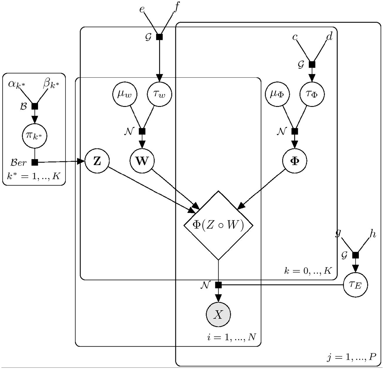
Graphical model representation of the infinite sparse independent component analysis. Observed variables are denoted with shaded nodes, while unobserved variables are shown as white nodes.

The complete model is expressed as:

\begin{matrix} \begin{array}{l} X \sim N (Φ (W \circ Z), diag (τ_{E_{1}}^{- 1}, \dots, τ_{E_{p}}^{- 1})) \\ τ_{E_{j}} \sim Gamma (g, h) \\ Φ_{j, k} \sim N (0, τ_{Φ_{j, k}}^{- 1}) \\ τ_{Φ_{j, k}} \sim Gamma (c_{j, k}, d_{j, k}) \\ W_{k, i} \sim N (0, τ_{W}^{- 1}) \\ τ_{W} \sim Gamma (e, f) \\ Z_{k^{*}, i}^{*} \sim Bernoulli (π_{k^{*}}) \\ Z_{0} = {[1, \dots, 1]}_{N} \\ π_{k^{*}} \sim Beta (\frac{α}{K}, \frac{β (K - 1)}{K}) \end{array} \end{matrix}

(3)

where $i = 1, \dots, N, j = 1, \dots, P, k = 0, \dots, K,$ and $k$ * $= 1, \dots, K$ . These priors apply regularization on the elements of $W$ and Φ using an automatic relevance determination (ARD) prior. Because strongly regularized elements are closed, but not equal to zero, we use the term pseudo-sparseness to distinguish this structure to the stricter sparseness imposed to $W$ by $Z$ . Considering $c = d = 1$ , the combination defines a super-Gaussian prior over the Φ elements, favoring source sparseness, and thus, independence. Considering gamma distribution for the priors over $τ_{W}$ , it corresponds to the Bayesian ridge prior for all the elements of the weight matrix $W$ .

Consistent estimation of the noise precisions ( $τ_{E}$ ), essential to determine the optimal number of latent components, is particularly challenging in a high dimensional setting and is a current hot research topic for matrix factorization noisy models (probabilistic PCA, FA, noisy ICA).¹⁴ Our empirical results from a simulation study confirmed this theoretical statement, highlighting that the model overfits the data, decomposing a part of the noise variance as additional irrelevant components (results not shown). To alleviate this issue, we standardized the input genes and fixed the noise precisions to $τ_{E} = 1$ , that is, to the variance of the centered and scaled gene expressions. This constraint indirectly regularizes the weight and source parameters, allowing identification of only strong signals, but may lead to false negatives in the hypergraph matrix identification (see results section).

Parameter inference and hyperparameter tuning

As the posterior computation using MCMC is notoriously slow when the number of parameters is high, we used variational Bayesian (VB) inference under the mean-field assumption to approximate the true posterior distribution.^15,16 We derived the variational evidence lower bound of the likelihood (ELBO) and the variational parameter update equations in Appendix A1.

For a computational purpose, we used the truncated beta process for the inference, with a maximum number of components noted $K_{m a x}$ .¹⁷ For all simulations and data analysis, we considered the prior hyperparameter values: $K_{m a x} = 100$ , $α = 1$ , $c = d = 1, e = f = 10^{- 6}$ .

Due to the lack of a simple analytical form of the conjugacy between the prior of the beta distribution and the beta distribution for its moments, we tuned the $β$ hyperparameter of the BBP using Bayesian optimization using the R package ParBayesianOptimization¹⁸ based on 6 initialization evaluations and 24 epochs (total of 30 evaluations). Considering $α = 1$ , we reparametrized $β$ as $μ = \frac{1}{1 + β}$ according to Ferrari and Cribari-Neto,¹⁹ which have support in the interval [0; 1] ( $μ = 0$ corresponding to $β = + \infty$ and $μ = 1$ to $β = 0$ ), to avoid restraining the support of $β \in [0; + \infty]$ with an a priori maximum value for the range of BO evaluation points.

Standard whitening ICA

We evaluated the ability of our method to reconstruct the matrix sparseness structures from simulated data sets in comparison with state-of-the-art algorithms. Due to computational issues for our larger scenario (time and/or memory), we used the standard whitening ICA model implemented in the ica²⁰ and the fastICA²¹ R packages, and pre-selected the components with eigenvalue higher than one. The eigenvalue criteria specifies that only components with eigenvalues larger than 1 should be preserved since each component should explain the variance of a single variable.

Results

The simulations, the parameter optimization, and the data visualization were performed using R software (version 3.6.0). The R codes and data are available on https://github.com/Oncostat/isgICA .

Synthetic data

Scenarios

We simulated synthetic datasets from equation (3), according to different scenarios (see Table 1) with $N = {100, 500}$ individuals, $P = {500, 1000, 5000}$ genes, and K $= {10, 30}$ components. The structure of Z was randomly generated to contain approximately 35% of ones. We considered 4 noise parameters ( ${σ_{E}}^{2} = {0.5, 1, 1.5, 2}$ ) to assess the impact of the signal-to-noise ratio.

Table 1.

Simulation scenarios. N, P, and ${σ_{E}}^{2}$ are the number of individuals, the number of genes and the noise variance respectively.

	N = 100	N = 500
K = 10 simulated components
P = 500	${σ_{E}}^{2} = {0.5, 1, 1.5, 2}$	${σ_{E}}^{2} = {0.5, 1, 1.5, 2}$
P = 1000	${σ_{E}}^{2} = {0.5, 1, 1.5, 2}$	${σ_{E}}^{2} = {0.5, 1, 1.5, 2}$
P = 5000	${σ_{E}}^{2} = {0.5, 1, 1.5, 2}$	${σ_{E}}^{2} = {0.5, 1, 1.5, 2}$
K = 30 simulated components
P = 500	${σ_{E}}^{2} = {0.5, 1, 1.5, 2}$	${σ_{E}}^{2} = {0.5, 1, 1.5, 2}$
P = 1000	${σ_{E}}^{2} = {0.5, 1, 1.5, 2}$	${σ_{E}}^{2} = {0.5, 1, 1.5, 2}$
P = 5000	${σ_{E}}^{2} = {0.5, 1, 1.5, 2}$	${σ_{E}}^{2} = {0.5, 1, 1.5, 2}$

For all scenarios, the elements of the source matrix Φ were generated for each component from Gaussian distributions with variance equal to one, and different means (from −3 to 3) to evaluate if the model may identify components with specific patterns, such as mainly positive or negative values, or both (for means closed to 0). Random blocks were generated to assign sparseness structure to this matrix presented by the Figure 5). The elements of the weight matrix W were drawn from a standard Gaussian distribution (mean = 0, variance = 1). We simulated 10 data sets for each scenario.

Performance criteria

As the standard ICA, our model is identifiable up to scaling, sign reversion, and column permutation.²² To evaluate the model reconstruction, we aligned the estimated components to the simulated ones using as a distance the mean of the absolute Pearson correlation coefficients of each pair of the column of the simulated source matrix $Φ$ and non-zero estimated columns of $\hat{Φ}$ . For the component $i$ of the simulated $Φ$ and the component $j$ of the estimated $\hat{Φ}$ ,this distance is estimated by $| \frac{cov (Φ_{., i}, \hat{Φ} ., j)}{σ_{Φ_{., i},} σ_{\hat{Φ}} ., j} |$ , which is invariant to the scaling and sign reversion. We used the Hungarian algorithm for an efficient re-ordering from this distance, using the HungarianSolver function of the RcppHungarian²³ R package.

The mean of the absolute Pearson correlation coefficients between the simulated Φ and Z°W and the column ordered $\hat{Φ}$ and Z°W was presented to assess the reconstruction of the source and weight matrix respectively.

According to the component ordering defined previously, the reconstruction of the sparseness structure of the weight matrix (except the baseline profile, ie, Z*) was assessed with the accuracy criterion, defined by: $\frac{T r u e o n e s + T r u e z e r o s}{N \times K} \in$ [0, 1].

Latent structure reconstruction

We first evaluated the ability of the algorithms to identify the number of components (Figure 3 and Table 2). The isgICA recovered the exact number of latent components in the majority of the simulations, but it underestimated the number in the lower dimension scenarios (P = 500), especially when the number of observations was low with respect to the number of component (N = 100, K = 30). This behavior was slightly more apparent when the noise variance was increased. The number of components selected with the classical whitening ICA using the eigenvalue method increased quickly with the dimension (P/N ratio) to the maximal number of components allowed by this approach (minimum between N-1 and P-1). It also slightly increased when the noise variance was raised in our algorithm.

Table 2.

Number of identified components (median [2.5%-97.5%] percentiles) using the eigenvalue method for the standard ICA and by the isgICA. N, P, and ${σ_{E}}^{2}$ are the number of individuals, the number of genes, and the noise variance respectively.

Model	${σ_{E}}^{2}$	N = 100			N = 500
Model	${σ_{E}}^{2}$	P = 500	P = 1000	P = 5000	P = 500	P = 1000	P = 5000
Eigen-value method		10 simulated components
	0.5	35 [19, 48]	66 [50, 79]	99 [99, 99]	28 [14, 43]	48 [29, 68]	412 [320, 457]
	1.0	54 [33, 66]	92 [82, 99]	99 [99, 99]	42 [20, 62]	82 [54, 106]	496 [470, 499]
	1.5	66 [46, 77]	99 [96, 99]	99 [99, 99]	56 [26, 76]	114 [79, 140]	499 [499, 499]
	2.0	74 [56, 84]	99 [99, 99]	99 [99, 99]	67 [33, 88]	139 [102, 167]	499 [499, 499]
		30 simulated components
	0.5	30 [27, 30]	31 [30, 34]	99 [99, 99]	30 [29, 32]	32 [30, 33]	48 [38, 95]
	1.0	31 [28, 32]	38 [32, 49]	99 [99, 99]	30 [29, 34]	32 [30, 38]	196 [167, 243]
	1.5	32 [30, 34]	56 [43, 70]	99 [99, 99]	31 [30, 35]	33 [31, 42]	338 [313, 371]
	2.0	36 [33, 39]	72 [60, 85]	99 [99, 99]	32 [30, 35]	38 [32, 48]	424 [404, 447]
isgICA method		10 simulated components
	0.5	10 [8, 10]	10 [10, 10]	10 [10, 10]	10 [10, 10]	10 [10, 10]	10 [10, 10]
	1.0	10 [8, 10]	10 [10, 10]	10 [10, 10]	10 [10, 10]	10 [10, 10]	10 [10, 10]
	1.5	10 [7, 10]	10 [10, 10]	10 [10, 10]	10 [10, 10]	10 [10, 10]	10 [10, 10]
	2.0	9 [6, 10]	10 [9, 10]	10 [10, 10]	10 [10, 10]	10 [10, 10]	10 [10, 10]
		30 simulated components
	0.5	11 [8, 14]	16 [13, 17]	20 [19, 22]	25 [20, 26]	29 [27, 30]	30 [29, 30]
	1.0	11 [9, 13]	16 [13, 16]	20 [19, 22]	22 [19, 24]	28 [27, 30]	30 [29, 30]
	1.5	11 [9, 13]	15 [13, 16]	20 [19, 22]	22 [18, 24]	28 [27, 30]	30 [29, 30]
	2.0	11 [9, 13]	15 [13, 16]	20 [18, 22]	20 [16, 23]	28 [27, 30]	30 [29, 30]

Figure 3.

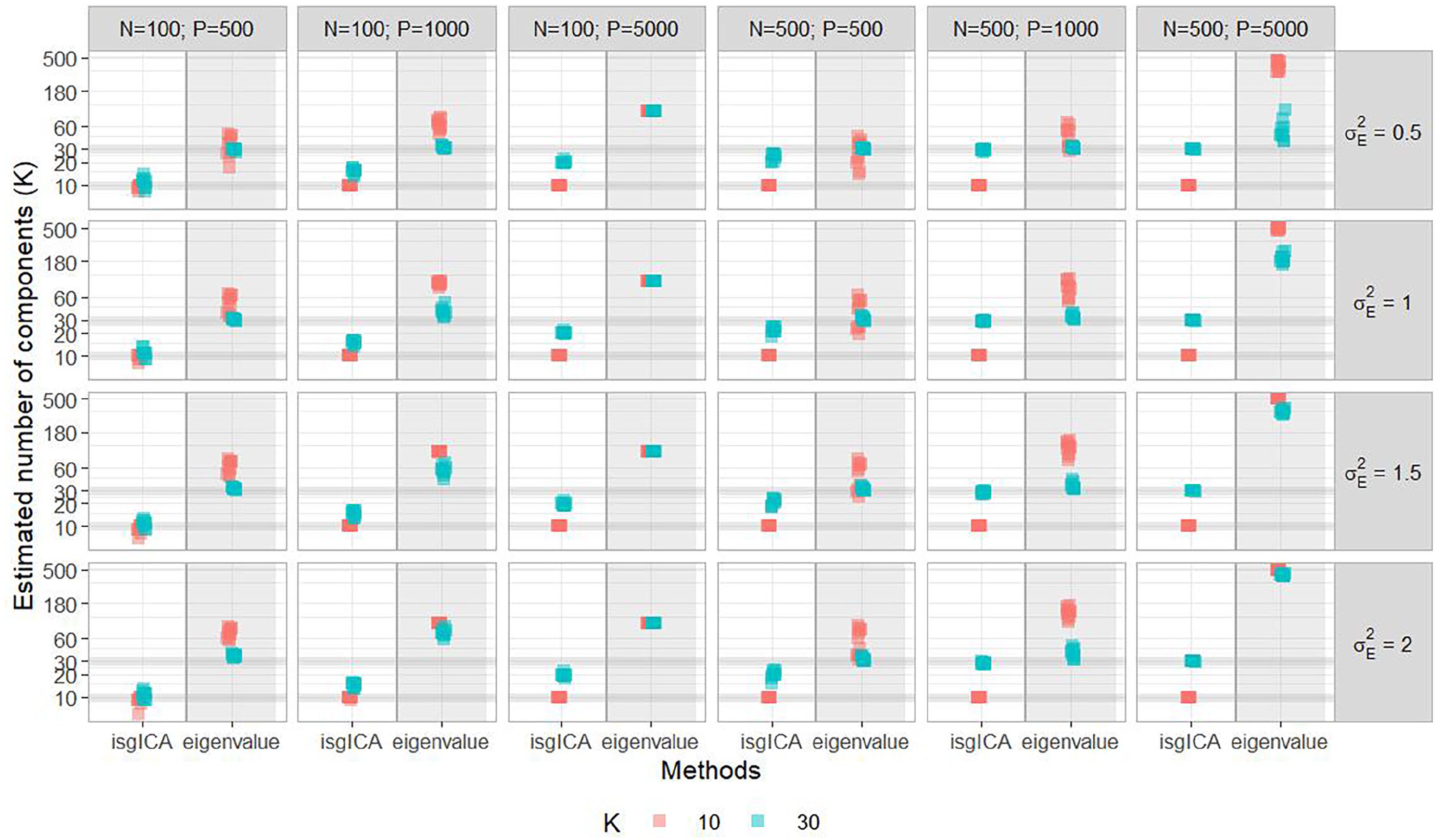
Reconstruction of the number of latent components between isgICA and the standard ICA using the eigenvalue criteria with 10 (red) or 30 (blue) simulated components (K). Each row corresponds to the scenarios with different noise variances ( ${σ_{E}}^{2}$ ) and each column corresponds to different dimensions (N individuals and P genes), for 10 simulations in each scenario.

Due to this over-decomposition using the eigenvalue method in the majority of the scenarios, the calculation of the reconstruction criteria for the ica and fastICA was not possible. In this case, we selected the 10 estimated components (or 30, according to the scenario) for which the source components were the most correlated to the simulated ones. We also performed an oracle sensitivity analysis, fixing a priori the number of components to the simulated ones for these 2 approaches, in order to have a comparison of their reconstruction to the blind reconstruction of the isgICA (see results in Appendix A2, Figures A1 and A2)

The isgICA outperformed the ica for the reconstruction of the source matrix (Φ) when the number of components was estimated using the eigenvalue method (Figure A1). This difference was less clear for the fastICA (correlation to simulated source matrix equal to .818 [.191, .934] (median [2.5%-97.5%] percentiles) for isgICA, .767 [.513,.982] for fastICA, and .189 [.0.28,.834] for ica), especially due to the lower performance of the isgICA in the scenarios with the lowest dimensions (N = 100/P = 500, and N = 500/P = 500). The performance of all methods decreased with the increase of the noise variance, but the isgICA was less impacted for high dimensional scenarios. The oracle fastICA and ica models presented in the majority of the scenarios a performance similar to the isgICA, excepting in the scenarios where the isgICA underperformed, that is, in the case of low dimension.

For all the scenarios, the isgICA outperformed the other methods for the reconstruction of the weight sparse matrices Z°W (mean absolute Pearson correlations equal to .968 [.225, .999] (median [2.5%-97.5%] percentiles) for isgICA, .453 [.194, .972] for the fastICA, .515 [.199, .983] for the ica), except for the scenarios with N = 100/500, P = 500 and K = 30. This result was explained by the over-decomposition using the eigenvalue method. Considering the oracle fastICA and ica models, the reconstruction performances were similar for all methods.

The isgICA results are summarized in the Figure 4. The ability of the isgICA to reconstruct the sparseness structure of the weight matrix ( $Z$ ) was accurate in the majority of the scenarios (accuracy >.8), but decreased when the number of parameters increased (ie, increasing P or K) to reach the simulated 35% of ones in the non-zeros components, corresponding to the accuracy of all-ones Z matrices. However, the good reconstruction of the weight sparse matrix (Z°W) in the high dimension scenarios indicates that this decrease of the accuracy for the strict sparseness is counterbalanced by the pseudo-sparseness induced by the ARD prior on $W$ .

Figure 4.

Reconstruction of the weight sparseness structure (Z), of the weight sparse matrix (Z°W) and sources matrix (Ф) according to different noise variances in rows with 10 (red) and 30 (blue) simulated components (K) and different dimensions (N individuals and P genes) in columns: the accuracy of the reconstruction of Z (first criteria), the mean absolute correlation of Z°W (second criteria) and the mean absolute correlation of Ф (third criteria), for 10 simulations in each scenario.

To illustrate the reconstruction ability of the isgICA, the Figure 5 shows the reconstruction of the sparse weight matrix (Z°W and the source matrix (Φ) for N = 500, P = 5000, K = 10 and ${σ_{E}}^{2} = 0.5$ . In this example, our approach was able to identify the correct number of non-zero components and reconstruct the accuracy of the weight sparseness matrix of .982, the sparse weight matrix with a mean absolute correlation of .999 and the source matrix with a mean absolute correlation of .873. As illustrated in the second row of the Figure 5, the ICA-based algorithm suffers from the standard ICA identifiability issues for the source matrix: the sign of the elements of some components may be reversed regarding the simulated one, and they may present higher values (scaling and sign identifiability issues). However, the ranking of the simulated and estimated values was highly correlated, allowing interpretation of the higher values of the source matrix as the most contributing genes to the components.

Figure 5.

Visual representation of the reconstruction of the weight sparseness structure (Z, top row, accuracy of .982) sparse weight structure (W°Z, middle row, correlation of .999) and sources(Ф, bottom row, correlation of .873) from a diagonal structure and with N = 500, P = 5000, K = 10 and ${σ_{E}}^{2}$ .

It can be noted that the ica method did not converge for 2.9% (14/480) simulations of the high dimension scenario (N = 500, P = 5000, K = 10) due to the large number of components identified using the eigenvalue method. Therefore, the result of this method is slightly overoptimistic and should be interpreted accordingly (including for the context of a real application).

The gain of precision for the (blind) matrix reconstruction and convergence rate for the isgICA relatively to the other methods came at the cost of a larger computational time relatively to the eigenvalue method (few minutes to several hours), that increases quickly with the dimension (Appendix A2, Figure A3).

Application: Early breast cancer data

We applied our method to publicly available gene expression data obtained from tumor biopsies in 614 breast cancer patients that were included in clinical trials of anthracycline-based chemotherapy,^24,25 available in the biospear R package.²⁶ The expression data of 22 277 probes (Affymetrix array) was preprocessed via frozen robust multiarray²⁷ and cross-platform normalization.²⁸ Probes were filtered if the interquartile range ⩽1. The remaining 1689 probes were standardized and then filtered with the package jetset²⁹ to retain a single probe by gene, resulting in a final dataset including the expression of 1063 genes. As in Belhechmi et al,³⁰ we mapped to probes to 3 molecular signatures with a prognostic effect in early breast cancer (Immune System, Proliferation, and Stroma invasion³¹) and one without (SRC activation signature³¹), all the other probes were categorized as “Others”.

Figure 6 presents the hypergraph matrix of the individual heterogeneity. The model identified 22 non-zero components (including the baseline profile).

Figure 6.

Hypergraph matrix of the individual heterogeneity (weight sparseness structure) extracted from the breast cancer dataset using the infinite sparse graphical independent component analysis with baseline profile. The model identified 22 components (including the baseline profile).

To investigate the molecular relevance of these results, we overcame the problems of sign and scale reversion by ranking the absolute source element values amongst each component to identify the most contributive genes to each identified molecular alterations. Figure 7 shows the distribution of the absolute values of the source matrix elements of each component according to the different breast cancer signatures. The proliferation-based signature, immune-system signature, and stroma-related signature seemed to be related to the components 2/5, 4/7/8/15, and 3, respectively. The SRC, which was picked as a “negative control” signature in Belhechmi et al,³⁰ was not straightforward to map to a particular molecular component.

Figure 7.

Distribution of the absolute value of the source matrix elements associated with the probes of genes associated with 3 molecular signatures with a prognostic effect in early breast cancer (GGI, Immune2, and Stroma2) and one without (SRC activation signature). All the other genes were categorized as “Others”. A proliferation-related signature, immune-related signature, and stroma-related signature seemed to be related to components 2/5, 4/7/8/15, and 3, respectively. The SRC was not related to one specific component.

Discussion

In this paper, we proposed a novel approach to characterize inter-patient heterogeneous molecular mechanisms. To our knowledge, this is the first approach that assumes that the molecular profile of each patient is a mixture of different molecular components, which can be shared with the other patients. We modeled these components as alterations from a baseline molecular component shared by all individuals, representing the mechanisms common to all patients, while the noise captures the individual molecular background. Assuming that each molecular component represents alterations of a molecular pathway or a group of related pathways, this approach may help us to understand molecular mechanisms and identify potential targets for drug development.

We illustrated the concept using a gene expression dataset of breast cancer tumor samples from patients included in clinical trials of anthracycline-based chemotherapy. The correspondence of the identified molecular profiles with known molecular pathways that play a prognostic role in early breast cancer (proliferation, immune system, and stroma pathway) suggests that our approach may help characterize the molecular context of particular subpopulations.

In the simulation study, our method was capable of blindly identifying the true number of components and their (sparseness) structures, up to scaling and sign reversion, which are well-known identifiability issues in standard ICA. To alleviate these issues, we proposed to use the absolute values of the source elements to identify the most contributive genes to each component for molecular interpretation. Comparing to 2 other popular ICA algorithms (fastICA and ica), our model better reconstructed blindly the number of components and the weight and source matrices, and had a similar performance when we a priori fixed the true number of components in these 2 algorithms.

Our algorithm was able to provide a better reconstruction performance of the weight sparse matrix (Z°W) than these 2 algorithms, even when the number of components was fixed a priori to the true number in the simulations. Our algorithm was also less sensitive to the increase of the dimension and the random noise variance. However, its lower performance in the lowest dimension scenarios suggests that the regularization may be too strong. Due to the well-known underestimation of the noise variance in high dimensional sparse models,³² we fixed it to 1 (ie, the variance of the classically standardized X if all component elements are equal to 0) to avoid the over-decomposition of the variance that results in an excess of components (not shown). This choice has an impact on the estimates because the noise variance is theoretically lower than 1 if the variance of X is explained by some components. That induces a too low signal-to-noise ratio resulting in posterior means of the component elements close to zero³² (ie, over-regularization), and therefore in an underestimation of the number of components. By contrast, the increase of the dimension decreases the influence of the noise variance, resulting in increasing of the posterior mean of the parameters that escape to the “spike” regularization pattern (Z) in the higher dimension scenarios (as reflected by the all-ones Z matrix posterior). However, the isgICA presents good performances in these settings as these parameters were regularized by the “slab” pattern (ARD prior), resulting in the observed pseudo-sparseness. In further research, the use of independent priors could be explored to alleviate the underestimation of the noise variance. But this approach based on non-conjugate priors requires complex algorithms for inference which could increase the computational time for a high dimensional data set.

As illustrated by our benchmark, the performance of our algorithm came at the cost of an important computational time that could be a practical limitation. A first next step will be to re-implement the current algorithm with GPU computation to scale-up to large datasets.

We showed that this approach is able to identify blindly components deviating from a baseline profile. Future research will focus on improvements for their identifiability and interpretability, including the integration of additional external information. We expect that some mixture weight components can reconstruct observed individual variables not considered by the model. It could be possible to extend this model, fixing the elements of some weight components to the values of observed individual variables, which may be relevant to explain the gene expressions (eg, gender, age, tumor stage). Beyond the adjustment for known characteristics, this extension could be used to perform differential analysis adjusted for unobserved individual characteristics. Moreover, while the bulk sequencing data results of a mixture of several elements (not only tumor cells, but also healthy tissue³³ or tumor microenvironment cells³⁴), other sources of data such as reference molecular profiles could be used to improve the identifiability and interpretability of the components. Another interesting way to integrate external information is to consider the patient characteristics as explanatory variable of the sparseness structure of the source matrix to model different states of the graph, as suggested by Wang et al.³⁵

The joint modeling of our isgICA and a clinical outcome, such as patient survival, could be of particular interest for precision medicine, favoring the identification of independent molecular profiles more specific to the patient prognostic. This extension will support the estimation of component/treatment interaction in the survival model to highlight pathways related to treatment response for the precision medicine context.

Finally, as proposed in the wide literature of omics data deconvolution methods, our approach may also be extended to other non-Gaussian omics data, such as count (raw RNAseq, proteomics) or binary (mutations) data using different link functions.

Conclusion

We developed an isgICA model with a baseline profile to characterize blindly the individual heterogeneity from this baseline profile in a high-dimensional setting. This approach illustrates a novel concept for the identification of composite molecular profiles which could be key to understanding the different mechanisms of disease and identify potential targets to develop new treatments.

Footnotes

Appendix

Funding:

The author(s) received no financial support for the research, authorship, and/or publication of this article.

Declaration of Conflicting Interests:

The author(s) declared no potential conflicts of interest with respect to the research, authorship, and/or publication of this article.

Author Contributions

SLR developed the model, and takes responsibility for the R programs and the accuracy of the data analysis. SLR drafted the manuscript; DD and SM contributed to a critical revision of the manuscript for important intellectual content, supervised the study equally, and gave final approval. All of the authors read and approved the final manuscript.

Data Availability

The breast cancer gene expression dataset is publicly available in the biospear R package. All code and associated data for the infinite sparse graphical independent component analysis with baseline profile is available on .

ORCID iD

Sarah-Laure Rincourt

References

Cunningham

Ghahramani

. Linear dimensionality reduction: survey, insights, and generalizations. J Mach Learn Res. 2015;16:2859-2900.

Yoshida

West

. Bayesian learning in sparse graphical factor models via variational mean-field annealing. J Mach Learn Res. 2010;11:1771-1798.

Feng

Heath

Jefferson

, et al. Hypergraph models of biological networks to identify genes critical to pathogenic viral response. BMC Bioinformatics. 2021;22:287.

West

Nevins

Marks

Spang

Zuzan

. Bayesian factor regression models in the “large p, small n” paradigm. In: Bernardo

Bayarri

Berger

Dawid

Heckerman

Smith

AFM

West

eds. Bayesian Statistics. Vol. 7. Oxford University Press; 2003:723-732.

Knowles

Ghahramani

. Nonparametric Bayesian sparse factor models with application to gene expression modeling. Ann Appl Stat. 2011;5:1534-1552.

Griffiths

Ghahramani

. Infinite latent feature models and the Indian buffet process. In: Proceedings of the 18th International Conference on Neural Information Processing Systems. NIPS-05. MIT Press; 2005:475-482.

Kabán

. On Bayesian classification with Laplace priors. Pattern Recognit Lett. 2007;28:1271-1282.

Carvalho

Polson

Scott

. Handling sparsity via the horseshoe. J Mach Learn Res. 2009;5:73-80.

Hjort

. Nonparametric Bayes estimators based on beta processes in models for life history data. Ann Stat. 1990;18:1259-1294.

10.

Paisley

Carin

. Nonparametric factor analysis with beta process priors. In: Proceedings of the 26th Annual International Conference on Machine Learning - ICML ‘09, Montreal, Quebec, Canada, Association for Computing Machinery; 2009; 777–784. doi:10.1145/1553374.1553474

11.

Hjort

Holmes

Müller

Walker

, eds. Bayesian Nonparametrics. Cambridge University Press; 2010.

12.

Gershman

Blei

. A tutorial on Bayesian nonparametric models. J Math Psychol. 2012;56:1-12.

13.

Hyvarinen

. Gaussian moments for noisy independent component analysis. IEEE Signal Process Lett. 1999;6:145-147.

14.

Bouveyron

Latouche

Mattei

. Exact dimensionality selection for Bayesian PCA. Scand J Stat. 2020;47:196-211.

15.

Beal

MJ.

Variational Algorithms for Approximate Bayesian Inference. 2003. https://cse.buffalo.edu/faculty/mbeal/papers/beal03.pdf

16.

Blei

Kucukelbir

McAuliffe

. Variational inference: a review for statisticians. J Am Stat Assoc. 2017;112:859-877.

17.

Paisley

Jordan

. A constructive definition of the beta process. Published online April 3, 2016. Accessed June 25, 2021. http://arxiv.org/abs/1604.00685

18.

Samuel

. ParBayesianOptimization: Parallel Bayesian Optimization of hyperparameters. Published online 2020. https://cran.r-project.org/web/packages/ParBayesianOptimization/index.html

19.

Ferrari

Cribari-Neto

. Beta regression for modelling rates and proportions. J Appl Stat. 2004;31:799-815.

20.

Helwig

. ica: Independent Component Analysis. Published online 2018. https://CRAN.R-project.org/package=ica

21.

Marchini

Heaton

Ripley

. fastICA: FastICA algorithms to perform ICA and projection pursuit. Published online 2019. https://CRAN.R-project.org/package=fastICA

22.

Sokol

H. Maathuis

Falkeborg

. Quantifying identifiability in independent component analysis. Electron J Stat. 2014;8:1438-1459.

23.

Kuhn

. The Hungarian method for the assignment problem. Nav Res Logist Q. 1955;2:83-97.

24.

Desmedt

Di Leo

de Azambuja

, et al. Multifactorial approach to predicting resistance to anthracyclines. J Clin Oncol. 2011;29:1578-1586.

25.

Hatzis

Pusztai

Valero

, et al. A genomic predictor of response and survival following taxane-anthracycline chemotherapy for invasive breast cancer. JAMA. 2011;305:1873-1881.

26.

Ternès

Rotolo

Michiels

. biospear: an R package for biomarker selection in penalized Cox regression. Bioinformatics. 2018;34:112-113.

27.

McCall

Bolstad

Irizarry

. Frozen robust multiarray analysis (fRMA). Biostatistics. 2010;11:242-253.

28.

Shabalin

Tjelmeland

Fan

Perou

Nobel

. Merging two gene-expression studies via cross-platform normalization. Bioinformatics. 2008;24:1154-1160.

29.

Birkbak

Gyorffy

Szallasi

Eklund

. Jetset: selecting the optimal microarray probe set to represent a gene. BMC Bioinformatics. 2011;12:474.

30.

Belhechmi

Bin

Rotolo

Michiels

. Accounting for grouped predictor variables or pathways in high-dimensional penalized Cox regression models. BMC Bioinformatics. 2020;21:277.

31.

Ignatiadis

Singhal

Desmedt

, et al. Gene modules and response to neoadjuvant chemotherapy in breast cancer subtypes: a pooled analysis. J Clin Oncol. 2012;30:1996-2004.

32.

Moran

Ročková

George

. Variance prior forms for high-dimensional Bayesian variable selection. Published online January 9, 2018. Accessed April 29, 2022. http://arxiv.org/abs/1801.03019

33.

Petralia

Wang

Peng

Yan

Zhu

Wang

. A new method for constructing tumor specific gene co-expression networks based on samples with tumor purity heterogeneity. Bioinformatics. 2018;34:i528-i536.

34.

Chen

Khodadoust

Liu

Newman

Alizadeh

. Profiling tumor infiltrating immune cells with CIBERSORT. Methods Mol Biol. 2018;1711:243-259.

35.

Wang

Baladandayuthapani

Kaseb

, et al. Bayesian edge regression in undirected graphical models to characterize interpatient heterogeneity in cancer. J Am Stat Assoc. 2022;0:1-14.

36.

Chen

Paisley

, et al. Bayesian inference of the number of factors in gene-expression analysis: application to human virus challenge studies. BMC Bioinformatics. 2010;11:552.

Complex Disease Individual Molecular Characterization Using Infinite Sparse Graphical Independent Component Analysis

Abstract

Keywords

Introduction

Methods

Infinite sparse graphical independent component analysis (isgICA)

Baseline profile and isgICA model

Complete model formulation

Parameter inference and hyperparameter tuning

Standard whitening ICA

Results

Synthetic data

Scenarios

Performance criteria

Latent structure reconstruction

Application: Early breast cancer data

Discussion

Conclusion

Footnotes

Appendix

Funding:

Declaration of Conflicting Interests:

Author Contributions

Data Availability

ORCID iD

References