Sage Journals: Discover world-class research

Abstract

We built a novel Bayesian hierarchical survival model based on the somatic mutation profile of patients across 50 genes and 27 cancer types. The pan-cancer quality allows for the model to “borrow” information across cancer types, motivated by the assumption that similar mutation profiles may have similar (but not necessarily identical) effects on survival across different tissues of origin or tumor types. The effect of a mutation at each gene was allowed to vary by cancer type, whereas the mean effect of each gene was shared across cancers. Within this framework, we considered 4 parametric survival models (normal, log-normal, exponential, and Weibull), and we compared their performance via a cross-validation approach in which we fit each model on training data and estimate the log-posterior predictive likelihood on test data. The log-normal model gave the best fit, and we investigated the partial effect of each gene on survival via a forward selection procedure. Through this we determined that mutations at TP53 and FAT4 were together the most useful for predicting patient survival. We validated the model via simulation to ensure that our algorithm for posterior computation gave nominal coverage rates. The code used for this analysis can be found at https://github.com/sarahsamorodnitsky/Pan-Cancer-Survival-Modeling.git, and the results are summarized at http://ericfrazerlock.com/surv_figs/SurvivalDisplay.html.

Keywords

Bayesian hierarchical modeling pan-cancer modeling survival analysis The Cancer Genome Atlas

Introduction

The recently completed The Cancer Genome Atlas (TCGA) program has provided a comprehensive molecular characterization of 33 cancer types from more than 10 000 patients, and the database remains a valuable public resource.¹ The different cancer types are generally defined by their tissue-of-origin. The project has revealed striking heterogeneity in the genomic and molecular profiles across patients within each cancer type. This heterogeneity is presented in several flagship publications (eg, see The Cancer Genome Atlas Network^2,3 and Verhaak et al⁴) in the form of molecularly distinct subtypes, and these subtypes often correlate with clinical end points. However, leveraging molecular heterogeneity for personalized risk prediction on a more granular scale is limited by the number of patients with reliable clinical data for each cancer type.⁵ Moreover, the effects of individual molecular biomarkers on survival or other clinical outcomes are often small, and thus predictive analyses within a single type of cancer are underpowered.⁶

In 2013, TCGA began the Pan-Cancer Analysis Project, motivated by the observation that “cancers of disparate organs reveal many shared features, and, conversely, cancers from the same organ are often quite distinct.”^7,8 The Pan-Cancer Analysis Project can also reveal differences in the effect of genomic changes across different cancer types, as demonstrated by the NOTCH gene family.⁷ This initiative has resulted in several studies across multiple cancer types that have revealed important shared molecular alterations for somatic mutations,⁹ copy number,¹⁰ messenger RNA,¹¹ and protein abundance.¹² If these potential biomarkers have similar clinical effects across multiple types of cancer, then predictive models that are estimated using pan-cancer data will have more power than models that are fit separately for each type of cancer. The TCGA Pan-Cancer Clinical Data Resource (TCGA-CDR)⁵ has facilitated pan-cancer models by curating and standardizing available data for 4 clinical outcomes (overall survival [OS], disease-specific survival, disease-free interval, or progression-free interval) across all 33 TCGA cohorts.

We propose and implement a novel Bayesian hierarchical framework to predict survival from multiple molecular predictors that are shared across multiple cancer types. An important feature of this approach is that it allows for borrowing information across models for each cancer type under the assumption that shared molecular predictors are likely to have a similar effect on survival prognosis, but it also allows sufficient flexibility for the same biomarker to have different effects depending on the type of cancer. Moreover, the Bayesian framework provides a principled way to incorporate prior information from other studies or cohorts, which is well-motivated given the vast body of literature on molecular biomarkers in cancer.

Using our proposed framework, we developed a pan-cancer predictive model for OS, using the somatic mutation profile of each tumor as the primary predictors of interest. We used OS because it is unambiguously defined and is available for almost all types of cancer, despite short follow-up times.⁵ We focus on somatic mutations because they play a critical role in the development of many cancer types,¹³ are available for all cohorts in the TCGA database, and are straightforward to compare across different tissues of origin. A pan-cancer analysis of somatic mutations across 12 different cancer types from TCGA revealed several genes that have frequent mutations across multiple types of cancer.⁹ Their analysis also considered the marginal effect of each gene on OS, via cox proportional hazards models for (1) each cancer type separately and (2) for a fully joint model with all cancer types together; our approach aims to compromise between these 2 strategies. For our application we consider the somatic mutation status of 50 genes, and survival data for 5698 patients comprising 27 different types of cancer. We evaluate and compare several different potential models via a robust cross-validation approach to assess predictive accuracy for this data set.

The rest of this article is organized as follows. In the “Methods” section, we discuss how the data were collected and our approach to filtering out cancer types and genes. We also describe our modeling framework, how we selected the survival distribution we chose to use in our analysis, and our Gibbs sampling algorithm to calculate the posteriors of the model parameters. In the “Results” section, we discuss the results of our model selection procedure and our approach to determining which genes were most predictive of survival. Using the results from these 2 processes, we show the resulting credible interval estimates of our parameters and display survival curves. In the “Discussion” section, we discuss our results and future work that builds on this study for pan-cancer survival modeling.

Methods

Data acquisition and processing

We acquired clinical data for each patient via the TCGA-CDR,⁵ which includes data for 33 cancer types and more than 11 160 patients. We acquired genome-wide somatic mutation data through the TCGA2STAT package for R,¹⁴ which gathers data from the Broad Institute GDAC Firehose. The curated mutation data were available for 27 305 genes and 5793 patients with a binary indicator for whether there was a somatic nonsilent mutation ( $0 = no$ , $1 = yes$ ) within the coding region of each gene.

We first matched the observations in the CDR data set with the mutation data obtained through TCGA2STAT. If any patients were present in one data set but not the other, that observation was removed from the study. We also removed any observations that had a negative survival time, a survival time entered as $0$ , or who were missing both a survival time and an entry for time-to-last-contact. We chose to eliminate 5 cancer types from our study due to high ( $> 90 %$ ) censoring rates, meaning patients survived longer than the duration of the study and their outcome status is unknown. These 5 types were pheochromocytoma and paraganglioma (PCPG), prostate adenocarcinoma (PRAD), testicular germ cell tumors (TGCT), thyroid carcinoma (THCA), and thymoma (THYM). The TCGA-CDR also caution against using OS as an end point for these cancer types, due to the lack of observed survival events. One other cancer type, mesothelioma (MESO), did not have any somatic mutation data available through the TCGA2STAT pipeline, so it was also omitted from our analysis. The 27 cancer types remaining in our study can be found in Table 1 with their corresponding sample sizes.

Table 1.

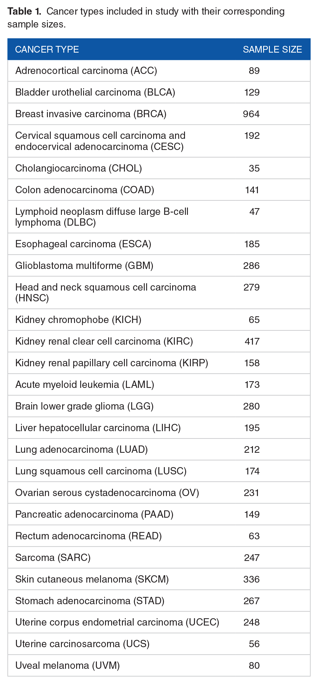
Cancer types included in study with their corresponding sample sizes.

Cancer type	Sample size
Adrenocortical carcinoma (ACC)	89
Bladder urothelial carcinoma (BLCA)	129
Breast invasive carcinoma (BRCA)	964
Cervical squamous cell carcinoma and endocervical adenocarcinoma (CESC)	192
Cholangiocarcinoma (CHOL)	35
Colon adenocarcinoma (COAD)	141
Lymphoid neoplasm diffuse large B-cell lymphoma (DLBC)	47
Esophageal carcinoma (ESCA)	185
Glioblastoma multiforme (GBM)	286
Head and neck squamous cell carcinoma (HNSC)	279
Kidney chromophobe (KICH)	65
Kidney renal clear cell carcinoma (KIRC)	417
Kidney renal papillary cell carcinoma (KIRP)	158
Acute myeloid leukemia (LAML)	173
Brain lower grade glioma (LGG)	280
Liver hepatocellular carcinoma (LIHC)	195
Lung adenocarcinoma (LUAD)	212
Lung squamous cell carcinoma (LUSC)	174
Ovarian serous cystadenocarcinoma (OV)	231
Pancreatic adenocarcinoma (PAAD)	149
Rectum adenocarcinoma (READ)	63
Sarcoma (SARC)	247
Skin cutaneous melanoma (SKCM)	336
Stomach adenocarcinoma (STAD)	267
Uterine corpus endometrial carcinoma (UCEC)	248
Uterine carcinosarcoma (UCS)	56
Uveal melanoma (UVM)	80

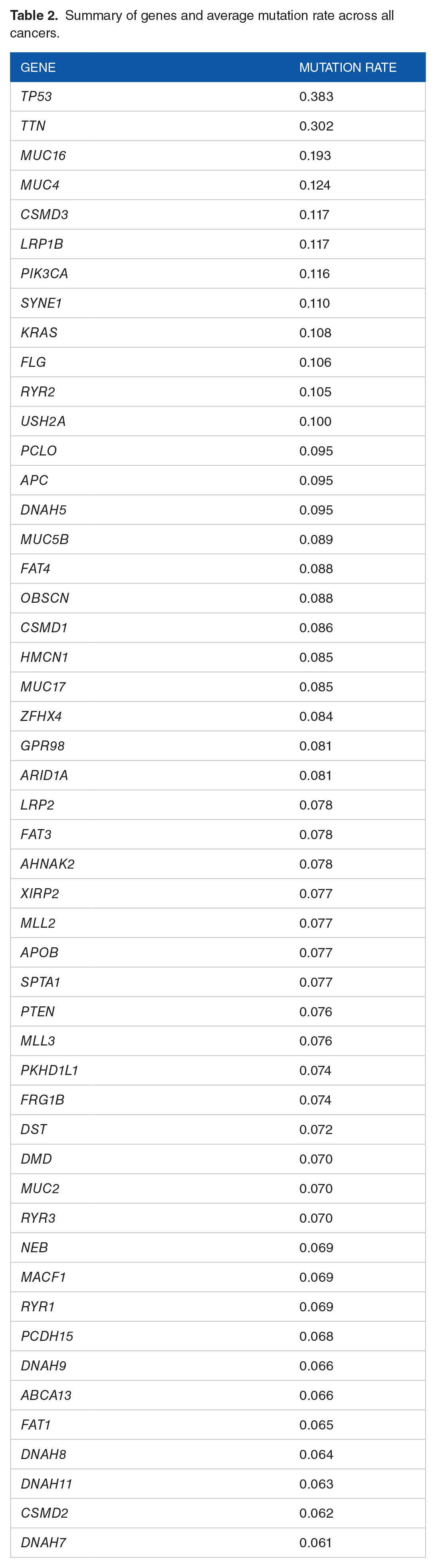
We filtered the genes based on average mutation rate across the 27 cancer types, selecting the top 50 mutated genes. To determine the average mutation rate, we calculated the mutation rate of each gene for each cancer type and took the average by gene across all cancers. In this way, each cancer type was weighted the same in calculating the mean mutation rate. This also ensured that each gene would be represented across most cancers, not just within a few. As a result, certain genes that are highly mutated in particular cancers but not in others were excluded. The genes we incorporated in our study can be found in Table 2 with their corresponding average mutation rates. In total, we used mutation data from 5698 patients.

Table 2.

Summary of genes and average mutation rate across all cancers.

Gene	Mutation rate
TP53	0.383
TTN	0.302
MUC16	0.193
MUC4	0.124
CSMD3	0.117
LRP1B	0.117
PIK3CA	0.116
SYNE1	0.110
KRAS	0.108
FLG	0.106
RYR2	0.105
USH2A	0.100
PCLO	0.095
APC	0.095
DNAH5	0.095
MUC5B	0.089
FAT4	0.088
OBSCN	0.088
CSMD1	0.086
HMCN1	0.085
MUC17	0.085
ZFHX4	0.084
GPR98	0.081
ARID1A	0.081
LRP2	0.078
FAT3	0.078
AHNAK2	0.078
XIRP2	0.077
MLL2	0.077
APOB	0.077
SPTA1	0.077
PTEN	0.076
MLL3	0.076
PKHD1L1	0.074
FRG1B	0.074
DST	0.072
DMD	0.070
MUC2	0.070
RYR3	0.070
NEB	0.069
MACF1	0.069
RYR1	0.069
PCDH15	0.068
DNAH9	0.066
ABCA13	0.066
FAT1	0.065
DNAH8	0.064
DNAH11	0.063
CSMD2	0.062
DNAH7	0.061

We considered the correlation of mutation status between genes across all cancers, for exploratory purposes and to investigate potential issues of multicollinearity for polygenic models. Figure 1 shows a pairwise correlation plot for all genes considered using mutation status across all patients included in this study. The Pearson correlation coefficients between genes were uniformly positive but relatively weak, ranging from $r = - . 07$ to $r = . 32$ . Almost all pairwise associations (96%) were significant at the .05 level based on a Fisher exact test for independence. The positive correlations were expected as the total mutation burden can vary across patients; however, the relative weakness of the correlations suggests that each individual gene may provide unique information and multicollinearity is not a concern. These correlations may change considerably if one were to consider only a single type of cancer or a subset of related cancers.

Figure 1.

Correlation plot for correlations between somatic mutation statuses across tissue types. Blank squares indicate nonsignificant correlation between 2 genes. Squares that contain a circle indicate significant correlations and the magnitude of the correlation is indicated by the color opacity.

Model

We propose a Bayesian hierarchical model for patient survival that incorporates binary mutation status variables and age across 27 cancer types. We centered the age covariate by subtracting out the average age for each cancer type. This reduces collinearity of the age coefficient with the intercept terms, ensuring that the estimated effect of age is not influenced by one cancer having generally older patients and another cancer having generally younger patients. The multilayer nature of our model allows the effect of a mutation at each gene to vary by cancer type while simultaneously inferring the mean and variance of these effects. Thus, the model facilitates the borrowing of information across cancer types by shrinking the estimated effects toward a common mean. Our model can also accommodate censored observations, as discussed in the following subsection. 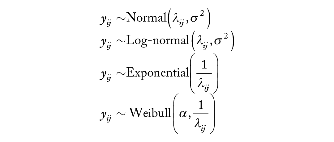We use the following notation in our framework: $y_{i j}$ is the (potentially censored) survival time for patient $j$ in cancer type $i$ , $j = 1, \dots, n_{i}$ , $i = 1, \dots, 27$ . The $x_{i j p}$ is the centered age if $p = 1$ and is the mutation status for gene $p - 1$ , $p = 2, \dots, 51$ . We consider 4 different likelihood models for survival:

\begin{array}{l} y_{i j} \sim Normal (λ_{i j}, σ^{2}) \\ y_{i j} \sim Log-normal (λ_{i j}, σ^{2}) \\ y_{i j} \sim Exponential (\frac{1}{λ_{i j}}) \\ y_{i j} \sim Weibull (α, \frac{1}{λ_{i j}}) \end{array}

For each likelihood we consider a hierarchical linear model for $λ_{i j}$ :

λ_{i j} = β_{i 0} + x_{i j 1} β_{i 1} + x_{i j 2} β_{i 1} + \dots + x_{i j 51} β_{i 51}

where $β_{i p}$ is the linear effect of age if $p = 1$ and mutation at gene $p - 1$ on survival if $p = 2, \dots, 51$ for a patient with cancer type $i$ . This approach extends commonly used parametric Bayesian survival models,¹⁵ and to complete the Bayesian framework we specify prior distributions for the unknown parameters. For the normal and log-normal models, we used an Inverse-Gamma $(0.01, 0.01)$ prior distribution for the residual variation of survival times within each cancer type, $σ^{2}$ . For the Weibull model, we used a Uniform $(0, 5)$ prior for the shape parameter, $α$ . Under the assumption that a mutation at one gene or an increase in 1 year of age may affect survival differently depending on the type of cancer, the linear effect of age and each mutation, $β_{i p}$ , was assumed to vary by cancer type. We assume

β_{i p} \sim Normal ({\tilde{β}}_{p}, λ_{p}^{2}) for p = 0, 51

where ${\tilde{β}}_{p}$ is the mean effect on survival across cancer types and $λ_{p}$ describes the extent to which the effects vary across the different types. Thus, ${\tilde{β}}_{i 0}$ gives the mean intercept and $β_{i 0}$ is an intercept that describes the baseline survival for type $i$ . Similarly, ${\tilde{β}}_{p}$ is the average effect on survival for age if $p = 1$ and for mutation at a gene if $p = 2, \dots, 51$ . For all coefficients and all models, we gave the mean effects independent and diffuse normal priors: ${\tilde{β}}_{p} \sim Normal {(0, 10000}^{2})$ . The parameters $λ_{p}^{2}$ are important because they indicate the degree of effect heterogeneity across cancer types; we used Inverse-Gamma $(0.01, 0.01)$ priors for each $λ_{p}^{2}$ .

Parameter estimation

Depending on the survival model, we employed a different approach to infer the posterior for model parameters. The log-normal and normal models were fit in R using an in-house Gibbs sampler. The sampler is described below; however, more details can be found in Appendix 1.

Initialize ${\tilde{β}}_{p}^{(0)}$ , $λ_{p}^{2 (0)}$ , $σ^{2 (0)}$ . Initialize all censored observations at their time of last contact.

For samples $t = 1, \dots, 20000$ , repeat the following steps:

Draw $β_{i p}^{(t)}$ from $P (β_{i p}^{(t)} | {\tilde{β}}^{(t - 1)}, λ^{2 (t - 1)}, σ^{2 (t - 1)})$ for $i = 1, \dots, 27$ and $p = 0, \dots, 51$ .

Draw $λ_{p}^{2 (t)}$ from $P (λ_{p}^{2 (t)} | β_{i p}^{(t)}, {\tilde{β}}^{(t - 1)})$ for $p = 0, \dots, 51$ .

Draw ${\tilde{β}}_{p}^{(t)}$ from $P ({\tilde{β}}_{p}^{(t)} | β_{i p}^{(t)}, λ_{p}^{2 (t)})$ for $p = 0, \dots, 51$ .

Draw $σ^{2 (t)}$ from $P (σ^{2 (t)} | β_{i p}^{(t)})$ for $i = 1, \dots, 27$ and $p = 0, \dots, 51$ .

Generate survival times for censored observations using $β_{i 1}^{(t)}, \dots, β_{i p}^{(t)}, σ^{2 (t)}$ .

● If assuming the data follows a normal distribution, generate survival times for censored observations from a normal distribution with mean β^(t)_i 0+ $β_{i 1}^{(t)} x_{i j 1} + \dots + β_{i 51}^{(t)} x_{i j 51}$ and variance $σ^{2 (t)}$ that is truncated at the time of last contact for observation $i j$ .

● If assuming the data follows a log-normal distribution, generate survival times from a normal distribution with mean $β_{i 0}^{(t)} + β_{i 1}^{(t)} x_{i j 1} + \dots + β_{i 51}^{(t)} x_{i j 51}$ and variance $σ^{2 (t)}$ that is truncated at the log of the time of last contact for observation $i j$ .

We ran the sampler for 20 000 iterations and used a 10 000 iteration burn-in to ensure convergence of the parameters. In Appendix 2 of this article, we describe how we validated this model fitting procedure.

Posterior samples for the exponential and Weibull models were obtained using the Just Another Gibbs Sampler (JAGS) software.¹⁶ For these models, we ran the sampler for the same number of iterations and employed the same burn-in as for the normal and log-normal models above. In all calculations based on the posteriors of our Gibbs sampler and our JAGS models, we thinned by every 10th iteration to speed up computing time and memory efficiency.

Model selection

To assess which of the normal, log-normal, exponential, and Weibull models was the best fit for the data, we calculated the log out-of-sample posterior predictive likelihood in a fivefold cross-validation procedure, as described below. Consider the $k th$ training-test partition of the data, $k = 1, \dots, 5$ such that $\vec{Y} = {{\vec{Y}}_{k}^{train}, {\vec{Y}}_{k}^{test}}$ . Let $p (y | X)$ be the probability distribution for survival time. On each training fold, we fit the model and generated posterior samples for each parameter. For each posterior sample after burn-in, we computed

P ({\vec{Y}}^{test} | Θ_{o}^{t}) = \prod_{\begin{matrix} (i, j) \\ uncensored \end{matrix}} p (y_{i j} | Θ_{o}^{t}) \prod_{\begin{matrix} (i, j) \\ censored \end{matrix}} \Pr (y_{i j} > y_{i j}^{c} | Θ_{o}^{t})

where $Θ_{o}^{t}$ is a vector of all the $t th$ -iteration posterior samples for the parameters of the probability distribution of survival and $y_{i j}^{c}$ is the censor time for the $j th$ patient in the $i th$ cancer type. After computing this quantity for each iteration, we computed an estimate of the out-of-sample posterior predictive likelihood:

\int P ({\vec{Y}}^{test} | Θ_{0}) P (Θ_{0} | {\vec{Y}}^{train}) d Θ_{0} \approx \frac{1}{T} \sum_{t = 1}^{T} P ({\vec{Y}}^{test} | Θ^{t})

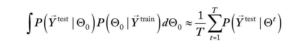
where T is the number of sampling iterations after burn-in and thinning. As stated previously, we chose to thin by every 10th iteration to ease computing time. As a result, this value was calculated based on 1000 Gibbs sampling iterations. After calculating the log-posterior predictive likelihood on each test fold, we took the average likelihood and compared the 4 models. More information on usage of the posterior predictive likelihood can be found in Vehtari and Ojanen.¹⁷

Forward selection

To assess the partial improvement of each gene in predicting survival, we constructed a forward selection approach that would allow us to see which genes were most important in predicting survival across all cancer types. In this way, we were able to determine the relative importance of each gene, and achieve a more parsimonious predictive model. For our forward selection approach, we used the same out-of-sample log-posterior likelihood metric described in the previous section on model comparison. Our forward selection method proceeded as follows:

Calculate the average log-posterior predictive likelihood for the null model (with age and cancer-type intercepts, but no genes) fit on each of the fivefolds.

For each gene, consider the model with only the intercept, age, and that gene included. Calculate the log-posterior predictive likelihood under this model using fivefold cross-validation.

(a) Select the gene that produced the model with the highest log-posterior predictive likelihood. Call this model $M_{1}$ .

(b) Compare the likelihood for this model with the null model; if the likelihood has increased, proceed by adding this gene to the model. Otherwise, stop.

For each remaining gene, add that gene separately to model $M_{1}$ and calculate the resulting mean log-posterior predictive likelihood using fivefold cross-validation.

(a)● Select from the resulting 2 gene models the gene that maximized the log-posterior likelihood. Call this model $M_{2}$ .

(b)● Compare the log-posterior likelihood for $M_{2}$ to $M_{1}$ . If the likelihood has increased, add the new gene to the model and proceed. Otherwise, stop.

Continue until the log-posterior predictive likelihood ceases to increase. At this point, the final model has been found.

The order of the genes added to the model depended on which genes maximized the posterior likelihood at each step. Once a final model had been found, we investigated the effects of each mutation on survival through credible interval plots and survival curves, described further in the “Results” section.

Results

Model selection

The results of the comparison described in the “Methods” section are shown in Table 3. We found that the log-normal model had the highest out-of-sample log-posterior likelihood out of the normal, exponential, and Weibull models. We assumed a log-normal distribution of survival for the remainder of our investigation.

Table 3.

Out-of-sample posterior predictive likelihood.

Model	Log-posterior likelihood
Log-normal	−3667.139
Normal	−3918.152
Exponential	−7053.263
Weibull	−6889.945

In this model, the coefficients are inferred by borrowing information across cancer types. However, we considered an analogous log-normal model in which the coefficients were inferred independently for each cancer type to compare with the model we selected here. We used the same uninformative prior on each coefficient as the one assumed for $\tilde{β} : β_{i j} \sim N {(0, 10000}^{2})$ . However, our in-house Gibbs sampler under this model failed to converge after 30 000 iterations for several coefficients. This demonstrates a drawback to not borrowing across cancer types as our proposed model does. We also considered a Cox proportional hazards model for each cancer type alone. Similarly, the result did not converge for several of the cancer types.

Forward selection

Table 4 displays the mean log-posterior predictive likelihoods for each step in the forward selection procedure. Every model is adjusted for patient age.

Table 4.

Results from forward selection procedure.

Covariates in model	Mean log-posterior likelihood
Age, no genes	−5014.895
Age, TP53	−1009.63
Age, TP53, FAT4	−1009.135
Age, TP53, FAT4, DNAH5	−1009.179

The log-posterior likelihood for the null model, meaning the model with only age as a predictor, was $- 5014.895$ . The model with TP53 added yielded a dramatic improvement, with a log-posterior likelihood value of $- 1009.63$ . The next gene to be added was FAT4, yielding a log-posterior likelihood of $- 1009.135$ . At this point, the posterior likelihood stopped improving. DNAH5 was last to be added, and the model with TP53, FAT4, and DNAH5 as predictors led to a log-posterior likelihood of $- 1009.179$ . We validated convergence of the forward selection procedure by running the process several times to ensure we obtained the same result. Across all 27 cancers, TP53 was mutated in an average of 38.3% of patients, the highest of all genes, and FAT4 in 8.8% (Table 2). The appearance of TP53 here is not surprising (see the “Discussion” section). However, we note that after the inclusion of TP53, the improvement in likelihood by FAT4 was marginal. This final model from our forward selection procedure served as our basis of exploration for subsequent analysis.

We also used our forward selection approach without including TP53 as a potential covariate to see what genes would be added. Our results are given in Table 5.

Table 5.

Results from forward selection procedure without TP53.

Covariates in model	Mean log-posterior likelihood
Age, no genes	−5014.895
Age, APOB	−1011.321
Age, APOB, ARID1A	−1011.694

Without including TP53 as a possible covariate, the first gene to be added was APOB, leading to a log-posterior likelihood of $- 1011.321$ . The addition of ARID1A on top of APOB led to the highest log-posterior likelihood of all genes at $- 1011.694$ though this metric ceased to increase at this point. Of the patients in our study, 7.7% had a mutation at APOB.

Credible intervals for model coefficients

To understand the magnitude and direction of the partial effect of age and a mutation at a gene on patient survival, we computed and visualized the $95 %$ credible interval based on posterior samples for each $β_{i p}$ . The intervals we show here were calculated from the multivariate log-normal model resulting from the forward selection procedure, with cancer type intercepts, age, TP53, and FAT4 included as predictors. The credible intervals for each $β_{i p}$ can be found in Table 6.

Table 6.

Credible intervals for model coefficients across each cancer type.

	Cancer	Intercept	Age	FAT4	TP53
1	ACC	(7.616, 8.347)	(−0.033, 0.007)	(−0.347, 0.67)	(−1.146, 0.020)
2	BLCA	(6.677, 7.379)	(−0.059, −0.005)	(−0.162, 0.732)	(−0.654, 0.180)
3	BRCA	(8.675, 9.021)	(−0.036, −0.015)	(−0.233, 0.771)	(−0.590, −0.037)
4	CESC	(7.757, 8.313)	(−0.030, 0.011)	(−0.226, 0.849)	(−0.558, 0.691)
5	CHOL	(6.402, 7.381)	(−0.047, 0.019)	(−0.745, 0.547)	(−0.537, 0.739)
6	COAD	(7.348, 8.134)	(−0.044, 0.010)	(−0.317, 0.614)	(−0.533, 0.377)
7	DLBC	(7.65, 8.721)	(−0.037, 0.031)	(−0.266, 0.812)	(−0.633, 0.765)
8	ESCA	(6.412, 7.284)	(−0.033, 0.005)	(−0.339, 0.539)	(−0.537, 0.351)
9	GBM	(5.657, 6.036)	(−0.043, −0.017)	(−0.462, 0.655)	(−0.053, 0.624)
10	HNSC	(7.225, 7.906)	(−0.042, −0.013)	(0.016, 0.957)	(−0.991, −0.222)
11	KICH	(8.662, 9.781)	(−0.074, −0.003)	(−0.308, 0.832)	(−1.000, 0.180)
12	KIRC	(7.724, 8.054)	(−0.052, −0.025)	(−0.443, 0.685)	(−0.858, 0.358)
13	KIRP	(7.941, 8.611)	(−0.016, 0.034)	(−0.406, 0.727)	(−0.893, 0.431)
14	LAML	(6.213, 6.666)	(−0.053, −0.025)	(−0.347, 0.843)	(−1.079, 0.028)
15	LGG	(7.676, 8.306)	(−0.072, −0.038)	(−0.282, 0.909)	(−0.369, 0.429)
16	LIHC	(6.761, 7.257)	(−0.024, 0.008)	(−0.154, 0.94)	(−0.668, 0.108)
17	LUAD	(7.188, 7.742)	(−0.032, 0.010)	(−0.174, 0.634)	(−0.603, 0.122)
18	LUSC	(6.549, 7.36)	(−0.054, −0.003)	(−0.229, 0.628)	(−0.189, 0.695)
19	OV	(6.963, 7.568)	(−0.048, −0.015)	(−0.280, 0.906)	(−0.334, 0.356)
20	PAAD	(6.302, 7.071)	(−0.039, 0.004)	(−0.476, 0.572)	(−0.588, 0.238)
21	READ	(7.376, 8.58)	(−0.056, 0.025)	(−0.196, 0.962)	(−0.556, 0.606)
22	SARC	(7.37, 7.844)	(−0.032, −0.004)	(−0.294, 0.842)	(−0.326, 0.386)
23	SKCM	(7.537, 7.927)	(−0.032, −0.011)	(−0.181, 0.425)	(−0.266, 0.515)
24	STAD	(6.495, 7.033)	(−0.034, 0.003)	(0.044, 0.796)	(−0.244, 0.452)
25	UCEC	(8.467, 9.097)	(−0.038, 0.008)	(0.061, 1.212)	(−0.786, 0.099)
26	UCS	(6.270, 7.518)	(−0.079, −0.007)	(−0.269, 0.835)	(−0.627, 0.537)
27	UVM	(7.268, 8.046)	(−0.069, −0.010)	(−0.303, 0.909)	(−0.856, 0.574)

Figure 2 displays the credible intervals across cancer types for each parameter in the model. Panel 2A compares the baseline survival across the different cancer types. Panel 2B reveals the generally deleterious effect of age on patient survival, as indicated by the highlighted orange intervals. For most of the cancers, an increase in age led to a decrease in survival; however, the extent to which age has an effect is not homogeneous or precisely identified for every cancer. For breast cancer (BRCA), the impact of age is more certain, indicated by a narrower credible interval, compared with the effect of age on patients with, eg, uterine carcinosarcoma. Similarly, Figure 2C shows the estimated effect of a TP53 mutation on survival across cancers, and the estimated effect was generally negative for most cancers. This, again, demonstrates a poorer prognosis for patients with a mutation at TP53. Breast cancer and head and neck squamous cell carcinoma (HNSC) had estimated TP53 effects with credible bounds entirely below 0, and adrenocortical carcinoma (ACC) was nearly entirely below 0. FAT4 mutation credible intervals (Figure 2D) appeared to be more positive than those of TP53, with some intervals entirely above 0.

Figure 2.

Credible intervals by cancer type for the intercept (panel A), Age effect (panel B), TP53 effect (panel C), and FAT4 effect (panel D).

Credible intervals for mean mutation effect

We also studied the credible intervals for the mean effect of each covariate. The mean effect for each predictor, ${\tilde{β}}_{p}$ , was assumed constant across cancer types and the individual effect by tumor varied around this mean. The results for ${\tilde{β}}_{p}$ are given in Table 7 and shown in Figure 3.

Table 7.

Credible intervals for mean of model coefficients.

Covariate	Mean effect
Intercept	(7.213, 7.870)
Age	(−0.037, −0.008)
FAT4 mutation status	(0.031, 0.480)
TP53 mutation status	(−0.316, 0.056)

Figure 3.

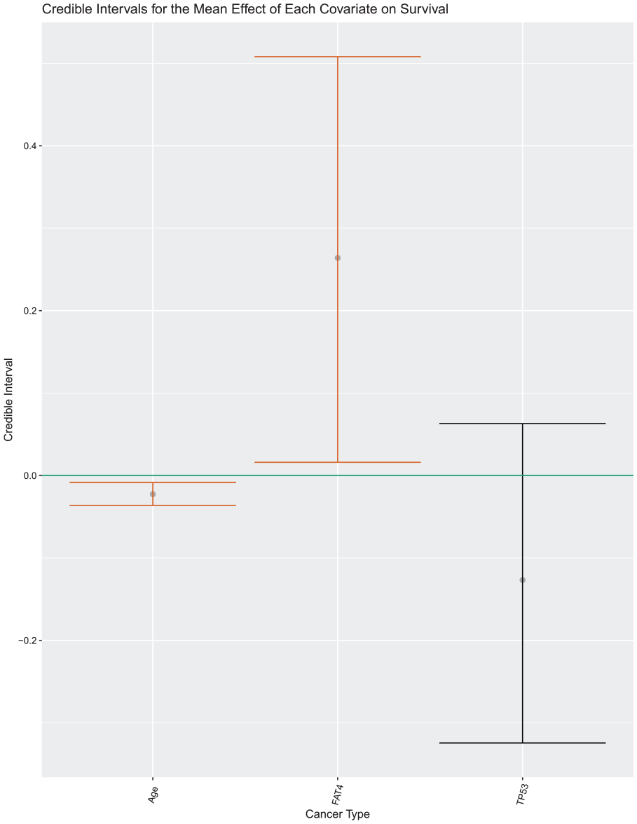
Visual display of the credible intervals for ${\tilde{β}}_{p}, p = 1, \dots, 3$ .

These results indicate the effect of each covariate averaged across cancers; therefore, if a predictor was more potent in one cancer and less so in another, this may not necessarily be represented in estimates for the mean effect. This substantiates why we chose to allow the effect of each covariate to differentiate by tumor type. The credible intervals for age and TP53 mutation status coincide with the $β_{i p}$ interval results as both had entirely negative or nearly entirely negative interval estimates for their respective means. The interval for FAT4 also coincides with the $β_{i p}$ intervals; however, its comparably large width demonstrates a lack of certainty on its effect with age and TP53 in the model.

Survival plots

To visualize the impact of age and a mutation at each of TP53 and FAT4, we show here survival curves computed based on each combination of predictor values. The full collection of survival curves, for any cancer type and any combination of predictors, are available online at http://ericfrazerlock.com/surv_figs/SurvivalDisplay.html. The plots displayed in Figure 4 are for a combination of covariates for patients with ACC, for which we had data on 89 tumors. In our data set, patients with ACC ranged in age from 14 to 83 years, with a median age of 49. The mutation rates for patients with ACC are as follows: 50.6% had no mutations in FAT4 or TP53, 10.1% had mutations in just FAT4, 19.1% had mutations at just TP53, and 4.49% had mutations in both. The impact of the negative coefficient of TP53 is demonstrated in these plots, as prognosis seems to worsen over 5 years if a patient has such a mutation. The deleterious effect of age is also visible, which is to be expected. The seemingly positive effect of FAT4 is also apparent, with calculated survival curves appearing higher compared with those for patients with no mutations at TP53 and FAT4.

Figure 4.

Survival curves under different covariate combinations for adrenocortical carcinoma with ages overlaid. Estimates for 30-year-old patients are shown in black, 50-year-olds in orange, and 80-year-olds in blue. The 95% error bounds are shown in dotted lines.

Discussion

In this article, we propose a novel Bayesian hierarchical model for survival of patients with cancer based on age and mutation status. This model is unique in its ability to allow the effect of each covariate to vary by cancer type. This framework is motivated by the assumption that similar genetic profiles may have similar, though not necessarily identical, effects on patient survival across tissues of-origin. This work may be extended to allow for other clinical covariates to be added to the model, such as stage and grade, and allows the user to adjust the effect of each predictor by cancer type as informed by prior knowledge.

To determine which genes were most important in survival prediction, we used a forward selection procedure that added TP53 and FAT4 to our model. The inclusion of TP53 led to a dramatic improvement in the model fit, while each additional gene reduced the log-posterior likelihood by a marginal amount. This indicates that TP53 is largely the most predictive, which is natural given its high mutation rate across cancer types (see Table 2). In particular, robust effects for TP53 were observed for BRCA and HNSC; the basal-like subtype for BRCA² and the human papilloma virus–negative subtype for HNSC¹⁸ are almost universally TP53-mutated and have relatively poor outcomes. Moreover, there is a vast literature on the mechanistic role of TP53 in cancer progression as an agent of DNA repair¹⁹ and in maintenance of genome integrity. It was also encouraging to see TP53 added to the model as it is considered a tumor driver gene.²⁰ FAT4 appears to be much less predictive than TP53, given its marginal increase in the log-posterior likelihood (from −1009.63 to −1009.135). It is of note that the credible intervals for coefficient in the model were largely positive, despite the existence of literature concluding FAT4 functions as a tumor suppressor.^21,22 A potential explanation is that mutations in FAT4 contribute to the development of certain cancers, but these cancers are comparatively less aggressive than those that arise from mutations in TP53 or other driver genes. An analysis without TP53 achieved comparable predictive performance under our hierarchical model via the inclusion of APOB, suggesting that even genes with lower mutation rates can improve performance. Using the most frequently mutated genes across genome sequencing cohorts often also includes known false positives. Comparing our list of genes with Bailey et al,²⁰ we found that 19 of 50 were on known false-positive lists. However, it was encouraging to see that these known false positives did not make the final survival model. However, our gene set also did not include some known tumor driver genes due to our approach of restricting the genes of interest to those with mutations across the pan-cancer cohort.

In addition, we considered the possibility of collinearity between mutation status variables, prompting us to investigate the correlation levels between variables across all cancer types (Figure 1). Based on this plot, we concluded mutation statuses across all cancer types were not highly associated. However, the results may look different if one is not considering the cancers in aggregate. With that in mind, we propose in future work sorting genes differently to meet the interest of the researchers, ie, exploring genes that are known to be highly mutated in a set of related cancers. In such an instance, it may be necessary to consider collinearity between variables and adjust accordingly.

We also assessed the predictive quality of our model by calculating survival curves for each cancer type based on combinations of age and mutation status based on our model. These plots demonstrated the largely negative effect of increasing age and a TP53 mutation and the less noticeable effect of FAT4. Irrespective of mutation status, the survival curves demonstrate the clear effect age has on survival prognosis, which does not come as much of a surprise. We created a web-based app that allows users to toggle with cancer types and predictors to see what 5-year prognosis is predicted to be. Such a tool may be interesting for academic purposes only.

In our study, we used the TCGA2STAT R package to import TCGA somatic mutation data due to its convenience in data dissemination, providing somatic mutation data in a ready-to-use format for statistical analysis. Although the package does offer convenience, we were not able to acquire data for MESO, which is available through the TCGA Multi-Center Mutation Calling in Multiple Cancers (MC3) data set and through the National Cancer Institute’s (NCI) Genome Data Commons. In the interest of ease of future replication of this study, using the TCGA2STAT data set may make it simpler for scientists to acquire the same data we used. We also did not distinguish the genes we used based on driver mutation status, false-positive status, or otherwise.

In future studies, it would be interesting to apply the model to a subset of the 27 cancer types we selected to group cancers that may be more similar in genetic nature or otherwise. This may elucidate genes unique to predicting patient survival outcome to specific cancer groupings. Interactions between covariates could also be included in the model to assess their relationship to OS. It would also be interesting to investigate alternate approaches to selecting genes to incorporate in the model, possibly incorporating prior knowledge on driver mutation status or false-positive status, or achieving variable selection through a sparsity inducing prior, as is done in Maity et al²³ using horseshoe priors.

Footnotes

Appendix 1

Appendix 2 Funding:

The author(s) disclosed receipt of the following financial support for the research, authorship, and/or publication of this article: This work was supported by the National Institutes of Health (NIH) National Cancer Institute (NCI) grant R21CA231214-01.

Declaration of Conflicting Interests:

The author(s) declared no potential conflicts of interest with respect to the research, authorship, and/or publication of this article.

Author Contributions

SS performed all analyses and drafted the manuscript. KAH provided helpful information and insight regarding the TCGA data and interpretation of the results. EFL conceived of the idea and developed the method with SS. All authors read and edited the manuscript.

ORCID iD

Eric F Lock

References

Hutter

Zenklusen

JC.

The Cancer Genome Atlas: creating lasting value beyond its data. Cell. 2018;173:283-285.

The Cancer Genome Atlas Network. Comprehensive molecular portraits of human breast tumors. Nature. 2012;490:61-70.

Cancer Genome Atlas Research Network. Comprehensive molecular profiling of lung adenocarcinoma. Nature. 2014;511:543-550.

Verhaak

Hoadley

Purdom

, et al. Integrated genomic analysis identifies clinically relevant subtypes of glioblastoma characterized by abnormalities in PDGFRA, IDH1, EGFR, and NF1. Cancer Cell. 2010;17:98-110.

Liu

Lichtenberg

Hoadley

, et al. An integrated TCGA Pan-Cancer Clinical Data Resource to drive high-quality survival outcome analytics. Cell. 2018;173:400-416.

Yuan

Van Allen

Omberg

, et al. Assessing the clinical utility of cancer genomic and proteomic data across tumor types. Nat Biotechnol. 2014;32:644-652.

Weinstein

Collisson

Mills

, et al. The Cancer Genome Atlas Pan-Cancer Analysis Project. Nature Genetics. 2013;45:1113-1120.

Hoadley

Yau

Hinoue

, et al. Cell-of-origin patterns dominate the molecular classification of 10,000 tumors from 33 types of cancer. Cell. 2018; 173:291-304.

Kandoth

McLellan

Vandin

, et al. Mutational landscape and significance across 12 major cancer types. Nature. 2013;502:333-339.

10.

Zack

Schumacher

Carter

, et al. Pan-cancer patterns of somatic copy number alteration. Nat Genet. 2013;45:1134-1140.

11.

Hoadley

Yau

Wolf

, et al. Multiplatform analysis of 12 cancer types reveals molecular classification within and across tissues of origin. Cell. 2014;158: 929-944.

12.

Akbani

PKS

Werner

, et al. A pan-cancer proteomic perspective on the Cancer Genome Atlas. Nat Commun. 2014;5:3887.

13.

Martincorena

Campbell

PJ.

Somatic mutation in cancer and normal cells. Science. 2015;349:1483-1489.

14.

Wan

Allen

Liu

TCGA2STAT: simple TCGA data access for integrated statistical analysis in R. Bioinformatics. 2015;32:952-954.

15.

Ibrahim

Chen

Sinha

Bayesian Survival Analysis. New York, NY: Springer Science+Business Media; 2013.

16.

Plummer

. JAGS: a program for analysis of Bayesian graphical models using Gibbs sampling. In Proceedings of the 3rd international workshop on distributed statistical computing, volume 124; Vienna, Austria, p. 10. https://www.r-project.org/conferences/DSC-2003/Proceedings/Plummer.pdf. Accessed February 4, 2020.

17.

Vehtari

Ojanen

A survey of Bayesian predictive methods for model assessment, selection and comparison. Statist Surv. 2012;6:142-228.

18.

The Cancer Genome Atlas Network. Comprehensive genomic characterization of head and neck squamous cell carcinomas. Nature. 2015;517:576-582.

19.

Olivier

Hollstein

Hainaut

TP53 mutations in human cancers: origins, consequences, and clinical use. Cold Spring Harb Perspect Biol. 2010;2: a001008.

20.

Bailey

Tokheim

Porta-Pardo

, et al. Comprehensive characterization of cancer driver genes and mutations. Cell. 2018;173:371-385.

21.

Cai

Feng

, et al. FAT4 functions as a tumour suppressor in gastric cancer by modulating Wnt/β-catenin signalling. Br J Cancer. 2015;113:1720-1729.

22.

Wei

Xiao

Song

Yuan

Luo

FAT4 regulates the EMT and autophagy in colorectal cancer cells in part via the PI3K-AKT signaling axis. J Exp Clin Cancer Res. 2019;38:112.

23.

Maity

Bhattacharya

Mallick

Baladandayuthapani

Bayesian data integration and variable selection for pan-cancer survival prediction using protein expression data. Biometrics. 2019. doi:10.1111/biom.13132.

24.

Lindley

Smith

AFM

. Bayes estimates for the linear model. J Roy Stat Soc B Met. 1972;34:1-41.

A Pan-Cancer and Polygenic Bayesian Hierarchical Model for the Effect of Somatic Mutations on Survival

Abstract

Keywords

Introduction

Methods

Data acquisition and processing

Model

Parameter estimation

Model selection

Forward selection

Results

Model selection

Forward selection

Credible intervals for model coefficients

Credible intervals for mean mutation effect

Survival plots

Discussion

Footnotes

Appendix 1

Appendix 2

Funding:

Declaration of Conflicting Interests:

Author Contributions

ORCID iD

References