A Method to Categorize 2-Dimensional Patterns Using Statistics of Spatial Organization

Abstract

We developed a measurement framework of spatial organization to categorize 2-dimensional patterns from 2 multiscalar biological architectures. We propose that underlying shapes of biological entities can be approached using the statistical concept of degrees of freedom, defining it through expansion of area variability in a pattern. To help scope this suggestion, we developed a mathematical argument recognizing the deep foundations of area variability in a polygonal pattern (spatial heterogeneity). This measure uses a parameter called eutacticity. Our measuring platform of spatial heterogeneity can assign particular ranges of distribution of spatial areas for 2 biological architectures: ecological patterns of Namibia fairy circles and epithelial sheets. The spatial organizations of our 2 analyzed biological architectures are demarcated by being in a particular position among spatial order and disorder. We suggest that this theoretical platform can give us some insights about the nature of shapes in biological systems to understand organizational constraints.

Introduction

Underlying shapes in biological entities are an important research area related to ontogenesis, evolution, and emergence of ecological patterns. Patterns are typically spatial heterogeneities extended in space, whereas forms are bounded and finite regions. ¹ Methodologically, patterns have been the main objective for some broadly used mathematical models and also have been understood as the main conceptual reference to approach biological shape.^2,3 Quantification of spatial order defines a statistical guideline to characterize, link, and use the concept of pattern and shape (eg, morphometrics). Despite the relevance of understanding the patterns and causal emergence of geometric order, traditional questions about patterns have not been involved with the quantification of spatial organization of them. Natural patterns are usually constructed by the spatial or temporal distribution of constitutive elements in a particular way, and often the global shape is considered as a consequence of that spatial organization. ⁴ Interestingly, a convergence of perspectives has been found in the analysis of ecological structures and the spatial organization of patterns in development. Based on the observation that fairy circles have a life cycle and life span and are biological entities competing for space-related resources, Zhang and Sinclair ⁵ speculated that fairy circles might be analyzed as epithelial architectures as has been done in previous works.^6–11

The existence of hexagonal lattices in both bees’ compound eyes and the honeycombs is an evidence of the packing problems in nature and their tendency to generate similar patterns, even at different scales. In a recent work, Berry et al ¹² found very similar shapes between molecular dynamics simulations of the nuclear pasta phases of dense nuclear matter that are expected deep in the crust of neutron stars and similar spiral-shaped ramps appearing in membrane-bound cellular organelles whose characteristic shapes are those being in the endoplasmic reticulum. They suggest that the very similar geometry of both systems may have similar coarse-grained dynamics and that the shapes are indeed determined by geometric considerations, independent of microscopic details. One interesting question emerging here is whether generic properties of spatial organization exist limiting the arrangement of those geometries. In fact, one of the most intriguing aspects of biology lies in the determination and organization of cellular types, organs, and structures in organisms which are associated with spatial or temporal heterogeneities or patterns,^13–16 which finally are geometries. However, a research focusing exclusively on the categorization of spatial arrangement of these biological geometries is far to be reached. Our main aim here is to introduce a method to categorize the spatial organization of 2-dimensional (2D) patterns. Two biological architectures are analyzed to reach this aim: epithelial topologies and Namibian fairy circles. (We are going to use the term architecture to define a global shape defined by polygonal accumulation. We adopt the word architecture to match the universal epithelial frequency [UEF; polygonal frequency of 49% of 6-sided polygons, 29% of 5-sided polygons, and 20% 7-sided polygons] of epithelial sheets and the self-organized geometric arrangement of the fairy circles of Namibia ⁵ which are called together biological architectures as our main case studies.) Regarding the epithelial tissues, several arguments have been put forward questioning the value of regularity associated with particular polygonality.^17–20 Sánchéz-Gutiérrez et al (2016) ¹⁸ describe how Voronoi diagrams are able to predict the diverse polygon distributions of any natural packed tissue. In that work, the authors demonstrate that Voronoi tessellations and the very different tissues analyzed share a restriction: the frequency of polygonal types correlates with the distribution of cell areas. Regarding this last point, our work is focused on the description of spatial organization in 2D patterns based on statistics of polygonal areas. In addition, we establish the relation between the frequency of polygonal types and cell areas to identify organizational conditions to understand the UEF. Some models predict that in the absence of cell sorting and migration, stochastic cell division would assemble into a distribution of polygonal cell shapes where hexagons, pentagons, and heptagons should be dominant in a UEF: nearly 46% of hexagons, 29% of pentagons, and 20% of heptagons.^6,7,10,11 Experimental data suggest that this polygonal distribution is common to the epithelial tissue of many metazoans.^11,21 Furthermore, the elsewhere proposed hypothesis of similar patterns of UEF with Namibian fairy circles would reflect geometric emergence by biological organization (self-organization). ²² As we can see, polygonal area variability and spatial organization can be strongly linked by a proper quantification of spatial heterogeneity.^23–25 Our definition of spatial heterogeneity is based on the unequal distribution of areas inside polygons. The breaking of spatial homogeneity or regularity in a lattice is called spatial heterogeneity, and we propose a statistical parameter to define quantitatively the spatial organization of 2D patterns. Associating this parameter with eutacticity (it has been shown in a previous work by Contreras-Figueroa et al ¹⁷ that eutacticity is closely linked with regularity and is a suitable measurement of spatial heterogeneity), we proved that there are exclusive biological pattern properties that are different from those found in nonbiological architectures. In fact, according to our proposed parameter, biological spatial organizations are characterized by being in a particular position among spatial order and disorder.

Intuitively, the degrees of freedom in a polygonal merge should increase proportionally to spatial heterogeneity. ²⁶ Statistically, the degrees of freedom are the number of values in a sample that are restricted to vary by a numerical constraint imposed. One important constraint in any spatial region is spatial homogeneity or regularity. Hence, the number of values associated with a group of areas inside a polygon would increase according to variability among those areas. The lack of spatial disparity among areas inside a region is regularity, and the increase of that disparity is spatial heterogeneity (Figure 1). This spatial heterogeneity can be translated in a parameter using the statistical definition of degrees of freedom. Our main hypothesis here is that there exists a parameter based on degrees of freedom of spatial distributions that can be used to characterize space organization in systems on multiple scales. The usage of this parameter might be applied to major questions concerning characterization of tissue organization and some other organismic perspectives (eg, tissue patterning, phenotypical convergence, conserved phenotypes, and evolutionary constraints).

Figure 1.

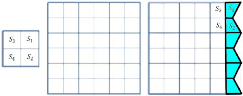
A square, its lattice, and the corresponding subareas. (A) A square is a locality associated with 4 subareas from 4 sublocalities $S_1,S_2,\dots ,S_N$ which are equal. By extension, (B) a global shape $\mathrm{\Gamma }$ with a partition such that all the sublocalities have equal subareas is regular. Statistically, this global shape $\mathrm{\Gamma }$ does not have any degrees of freedom. (C) The right figure shows a global shape that has increased its degrees of freedom as the set of blue areas (right side) defined by sublocalities $S_1\mathrm{and}{S}_2$ are smaller than those of $S_3\mathrm{and}{S}_4$ in 3 of the 9 localities. Disparity of areas inside localities is increased as $S_1\mathrm{and}{S}_2$ are different from $S_3\mathrm{and}{S}_4$ .

Section “Methods” shows the statistical basis of our work: we introduce 2 statistical parameters defining the variability of areas inside a lattice, which will define particular spatial configurations. Section “Mathematics of eutacticity” is about mathematics of eutacticity considering important previous references.^17,26 Our numerical proof in section “Numerical proof associating eutacticity and standard deviation of dispersion mean of a module” will define the amplitude of spatial variability of elements in a lattice, called modules, showing the association between eutacticity with our statistical argument. In section “Generation of global form $\mathrm{\Gamma }$ ,” the method to build global forms called sets gamma is shown, and the statistical categorization of them is given.

Methods

To establish a proper measure of spatial organization, we start by defining a global shape $\mathrm{\Gamma }$ . Given a spatial domain $R$ in $R^2$ , we define $R$ as $R={\cup }_{i=1}^{\gamma }{L}_i$ , where $L_i$ is a convex regular or irregular polygon which will be called a locality and $\gamma$ is a natural number. Each locality is constituted by a subset of a given number of $N_i$ sublocalities, $S_{i1},S_{i2},\dots ,S_{i_{Ni}}$ , such that $L_i={\cup }_{j=1}^{N_i}{S}_{ij}$ . Let $A_{ij}=area(S_{ij})$ be the area of each sublocality. If $A_{ij}=A_{ik}\forall k,j$ , then $L_i$ is regular (Figure 1). In contrast, if $\exists j\ne k$ such that $A_{ij}{A}_{ik}$ , then $L_i$ is not regular. Therefore, let $A_i={\displaystyle {\sum }_{j=1}^{N_i}{A}_{ij}}$ be the sum of all the associated areas of every locality; this set determines $\mathrm{\Gamma }=\left\{A_i\right\}$ . The average of areas of a locality $L_i$ is ${\overline{A}}_i=(1/N_i){\displaystyle {\sum }_{j=1}^{N_i}{A}_{ij}}$ , and ${\mathrm{\sigma }}_i=\sqrt{(1/N_i-1){\displaystyle {\sum }_{j=1}^{N_i}{(A_{ij}-{\overline{A}}_i)}^2}}$ is the standard deviation of each locality. It is important to say that if ${\mathrm{\sigma }}_i=0\Rightarrow A_{ij}=A_{ik}\forall j,k$ . Accordingly, to establish a global measure for regularity of tessellations, we define a mean of global dispersion (MGD) and global dispersion of gamma (GDG) as follows:

$${\overline{\mathrm{\sigma }}}_{{\gamma }_1}=\frac{1}{\gamma }{\displaystyle \sum _{i=1}^{\gamma }{\mathrm{\sigma }}_i}$$

(1)

and

$${\mathrm{\sigma }}_{\mathrm{\Gamma }}=\sqrt{\frac{1}{\gamma -1}{\displaystyle \sum _{i=1}^{\gamma }{({\mathrm{\sigma }}_i-{\overline{\mathrm{\sigma }}}_{{\gamma }_1})}^2}}$$

(2)

The MGD and the GDG will be considered as our main references to define the regularity of a form and hence determine its spatial organization. However, to provide a practical measure of regularity using the statistical framework described, we conduct a numerical proof relating MGD and GDG to a mathematical measure called eutacticity in section “Numerical proof associating eutacticity and standard deviation of dispersion mean of a module.” Eutacticity has been associated with regularity in terms of spatial distribution of areas. ⁷ Although eutacticity has been proposed as a measure of regularity and appears to be a meaningful property to understand spatial order, ¹⁷ it has not been properly explained as a source of information to characterize 2D patterns statistically, establishing particular limits for biological organizations. As a result of our numerical proof, we realize that the statistical framework given before provides an explanation of the meaning of the eutacticity parameter. ²⁶ A brief explanation of eutacticity is included in section “Mathematics of eutacticity” before the proof.

Mathematics of eutacticity

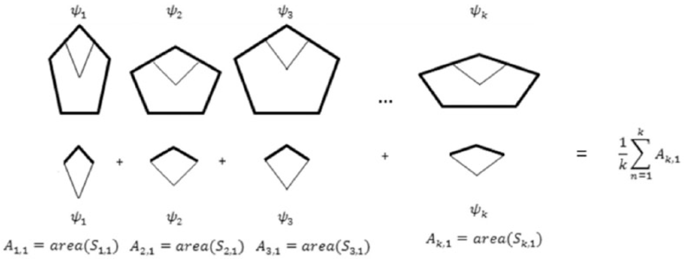
A star $\psi$ is a set of $n$ vectors $\{{\mathbf{u}}_1,{\mathbf{u}}_2,\dots ,{\mathbf{u}}_n\}$ with a common origin in an N-dimensional space $(R^N)$ . It is eutactic if it can be obtained by projecting an orthogonal set. Eutacticity is sharply linked with regularity considering that a given polygon, polyhedron, and, in general, polytope can be associated with a star of vectors (pointing to the center to the vertexes), and it has been demonstrated that stars linked with regular polytopes are highly eutactic. ²⁶ A good numerical criterion for obtaining the eutacticity of a star, suitable for dealing with experimental measurements, was proposed by Coxeter, ²⁷ and it is as follows. Let $B$ be the matrix whose $N$ columns are the components of the vector composing a star $\psi$ , with respect to a given fixed orthonormal basis of $R^2$ . The star is eutactic if and only if

$$\epsilon =\frac{Tr\left(S\right)}{\sqrt{Tr\left(SS\right)}\sqrt{2}}=1$$

(3)

where $S=B{B}^T$ ; $Tr$ denotes the trace and the superindex $T$ denotes the transpose. Note that the parameter $\epsilon$ is capable of indicating the degree of eutacticity of the star represented by $B$ : if it is not strictly eutactic $(\epsilon =1)$ , then this quantity is closer to 1 if the star has a high eutacticity. In our particular case of planar stars, it can be proved that

$$\frac{1}{\sqrt{2}}⩽\epsilon ⩽1$$

(4)

As already mentioned, the strategy was to associate a particular polygon or locality $L_i$ with a star $\psi$ and measure its eutacticity by means of equation (7). From this definition, a measure of spatial heterogeneity could be proposed, and it was used to measure the regularity of any polygon in a mosaic pattern or global form $\mathrm{\Gamma }$ , using sublocality areas. Therefore, we need to prove that while the closer $\epsilon$ is to 1, the more regular the star is (next section). Our hypothesis is that the higher the eutacticity, the partition of the space is more homogeneous (ie, the area variability of the sublocality decreases). Lower values of eutacticity imply unequal partition of the space or more area variability increasing spatial heterogeneity. According to equations (1) and (2), the variability defining regularity must occur inside localities, which will globally give a hint for determining degrees of freedom statistically. To support statistical variation between highly regular stars or highly eutactic stars in contrast to nonregular stars, we need to define spatial variability between 2 experimental groups, highly eutactic and less eutactic stars, and polygons associated with them.

Numerical proof associating eutacticity and standard deviation of dispersion mean of a module

The algorithms used in this section are found in a study by López-Sauceda et al. ²⁶ We will show, in this section, that eutacticity is an important parameter measuring spatial arrangement using the module concept to support the statistical framework of the first section. In the same context, we prove that eutacticity conveys a practical measure of spatial variation inside localities whose $\epsilon$ parameter accounts for MGD and GDG. Spatial organization is the fundamental property to figure out regularity using polygons, and a partition of localities $L_i$ into sublocalities $S_{i1},S_{i2},\dots ,S_{i_{Ni}}$ is proposed using Voronoi tessellations according to a proper algorithm in a study by López-Sauceda et al. ²⁶ The purpose of the study by López-Sauceda et al ²⁶ was the verification of spatial distribution of areas inside localities by comparing highly eutactic and no highly eutactic stars. Therefore, there were 2 experimental groups: ${\psi }_a$ representing highly eutactic stars $\epsilon =1({\psi }_1)$ and ${\psi }_b$ representing nonhighly eutactic stars $\epsilon =0.8({\psi }_2)$ . The properties of stars $\psi$ from any of these 2 groups are as follows. There will be ${\psi }_1,{\psi }_2,\dots ,{\psi }_k$ stars such that (1) they have the same eutacticity $\epsilon$ ; (2) any of them has the same number of vectors $\nu$ ; (3) they are random stars, even though any of them has the same eutacticity value (all of them are geometrically different); and finally, (4) stars ${\psi }_1,{\psi }_2,\dots ,{\psi }_k$ are the building blocks to construct localities $L_1,L_2,\dots ,L_k$ with the number of sublocalities associated with same number of vectors $v$ . In fact, according to property (2), $N_i=N_j=v,\forall i,j$ occurs, which is an important condition to continue with a formal definition of module. Intuitively, a module is a summation of particular sublocalities from many localities, and it will be used to contrast 2 arbitrary values of $\epsilon$ (Figure 2). According to López-Sauceda et al, ²⁶ let us assume that the areas $A_{i,j}$ associated with sublocalities of the 2 groups of stars $\epsilon =1({\psi }_1),\epsilon =0.8({\psi }_2)$ have 2 crucial components: (1) the eutacticity $\epsilon$ of the star $\psi$ and (2) a set of random points ${\omega }_{m,n}$ defining the associated areas $A_{i,j}$ . It is important to highlight that $L_1,L_2,\dots ,L_k$ depend on ${\psi }_1,{\psi }_2,\dots ,{\psi }_k$ (property 4 of stars $\psi$ ). According to this, ${\psi }_1,{\psi }_2,\dots ,{\psi }_k$ are associated with ${\omega }_{m,n}$ . In that sense, let us name the stars ${\psi }_{1,j}^{{\omega }_{1,n}},{\psi }_{2,j}^{{\omega }_{2,n}},\dots ,{\psi }_{k,j}^{{\omega }_{k,n}}$ where $j$ represents the particular sublocality and $n$ is the set of random points $n=1,\dots ,\alpha$ . So, ${\omega }_{m,i}\ne {\omega }_{m,j}$ for every $ij$ . According to this, $m=1,\dots ,k$ is a simple tag to associate star $k$ with ${\omega }_k$ and subsequently with a set $\alpha$ of random points, and the associated areas are $A_{1,j}^{{\omega }_{1,n}},A_{2,j}^{{\omega }_{2,n}},\dots ,A_{k,j}^{{\omega }_{k,n}}$ . Therefore, the module for a particular sublocality is defined using the average of areas of that locality. Modules for particular sublocalities of 2 experimental groups of stars $\epsilon =1({\psi }_1),\epsilon =0.8({\psi }_2)$ are built to contrast its sublocality area variations.

Figure 2.

Construction of a module from $k$ stars. A module is an average derived from an area summation of a particular sublocality (eg, sublocality 1) from $k$ stars $\psi$ with a constant value $\epsilon$ . Stars ${\psi }_1,{\psi }_2,\dots ,{\psi }_k$ are the building blocks to construct localities $L_1,L_2,\dots ,L_k$ . This process is applied to build modules of 2 experimental groups of stars ${\psi }_a$ and ${\psi }_b$ .

For instance, assuming that we need to establish an analysis of module 1 exclusive for sublocality 1 in a locality of $j$ sublocalities, we have Table 1.

Table 1.

Calculation of a module for sublocality 1.

	Set of random points ${\omega }_{m,n}$ defining the associated areas Ai,j for sublocality 1 (algorithm defined in Aguilar-Hidalgo et al 14 )					Summation of areas for star ${\psi }_k$
Stars	${\omega }_{1,1}$	${\omega }_{1,2}$	. . .	${\omega }_{1,\alpha }$
${\psi }_1$	$A_{1,1}^{{\omega }_{1,1}}$	$A_{1,1}^{{\omega }_{1,2}}$	. . .	$A_{1,1}^{{\omega }_{1,\alpha }}$	⇒	$\frac{1}{\alpha }{\displaystyle {\sum }_{n=1}^{\alpha }{A}_{1,1}^{{\omega }_{1,n}}}$
${\psi }_2$	$A_{2,1}^{{\omega }_{2,1}}$	$A_{2,1}^{{\omega }_{2,2}}$	. . .	$A_{2,1}^{{\omega }_{2,\alpha }}$	⇒	$\frac{1}{\alpha }{\displaystyle {\sum }_{n=1}^{\alpha }{A}_{2,1}^{{\omega }_{2,n}}}$
${\psi }_k$	$A_{k,1}^{{\omega }_{k,1}}$	$A_{k,1}^{{\omega }_{k,2}}$	. . .	$A_{k,1}^{{\omega }_{k,\alpha }}$	⇒	$\frac{1}{\alpha }{\displaystyle {\sum }_{n=1}^{\alpha }{A}_{k,1}^{{\omega }_{k,n}}}$

The summation ∑ of module 1 derived from sublocality 1 in a locality of $j$ sublocalities, $k$ stars, and $\alpha$ set of random points is defined as follows:

$$\frac{1}{\alpha }\left({\displaystyle \sum _{n=1}^{\alpha }{A}_{11}^{{\omega }_{1n}}}+{\displaystyle \sum _{n=1}^{\alpha }{A}_{21}^{{\omega }_{1n}}}+\cdots +{\displaystyle \sum _{n=1}^{\alpha }{A}_{k1}^{{\omega }_{1n}}}\right)$$

(5)

Therefore, the average for module 1 is determined as follows:

$$\begin{array}{l}{\overline{A}}_{{\mu }_1}=\frac{1}{\alpha k}{\displaystyle \sum _{i=1}^k{\displaystyle \sum _{n=1}^{\alpha }{A}_{i,1}^{{\omega }_{i,n}}}}\\ {\mathrm{\sigma }}_{{\mu }_1}=\sqrt{\frac{1}{\left(\alpha -1\right)\left(k-1\right)}{\displaystyle \sum _{n=1}^{\alpha }{\displaystyle \sum _{i=1}^k{\left(A_{i1}^{{\omega }_{in}}-{\overline{A}}_{\mu }\right)}^2}}}\end{array}$$

(6)

In general, for any sublocality $A_{i,j}^{{\omega }_{i,n}}$ linked to the star $S_i$ , if we want the average of every star and the average of every set of random points of module $A_{{\mu }_j}$ , it is given as follows:

$$\begin{array}{l}{\overline{A}}_{{\mu }_j}=\frac{1}{\alpha k}{\displaystyle \sum _{i=1}^k{\displaystyle \sum _{n=1}^{\alpha }{A}_{i,j}^{{\omega }_{i,n}}}}\\ {\mathrm{\sigma }}_{{\mu }_j}=\sqrt{\frac{1}{\left(\alpha -1\right)\left(k-1\right)}{\displaystyle \sum _{i=1}^{\alpha }{\displaystyle \sum _{n=1}^k{\left(A_{i,j}^{{\omega }_{i,n}}-{\overline{A}}_{{\mu }_j}\right)}^2}}}\end{array}$$

(7)

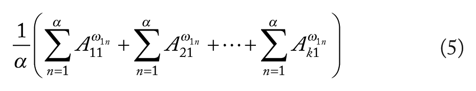
Now fix a star and obtain the average of areas and standard deviation of this locality by summation over $\alpha$ random set of points:

$$\begin{array}{l}{\overline{A}}_{{\mu }_j}\left(S_i\right)=\frac{1}{\alpha }{\displaystyle \sum _{n=1}^{\alpha }{A}_{i,j}^{{\omega }_{i,n}}}\\ {\mathrm{\sigma }}_{{\mu }_j}\left(S_i\right)=\sqrt{\frac{1}{\alpha -1}{\displaystyle \sum _{n=1}^{\alpha }{\left(A_{i,j}^{{\omega }_{i,n}}-{\overline{A}}_{{\mu }_j}\left(S_i\right)\right)}^2}}\end{array}$$

(8)

The average of these standard deviations performing summation over the $k$ stars is as follows:

$${\overline{\mathrm{\sigma }}}_{{\mu }_j}=\frac{1}{k}{\displaystyle \sum _{i=1}^k{\mathrm{\sigma }}_{{\mu }_j}\left(S_i\right)}$$

(9)

where $j$ is the dispersion mean of module which will have the following final standard deviation of dispersion mean of module:

$${\mathrm{\sigma }}_{S\mu }=\sqrt{\frac{1}{\left(k-1\right)}{\displaystyle \sum _{i=1}^k{\left({\mathrm{\sigma }}_{{\mu }_j}\left(S_i\right)-{\overline{\mathrm{\sigma }}}_{{\mu }_j}\right)}^2}}$$

(10)

Figure 3 shows how this standard deviation reflects the spatial variation of areas inside a given number of stars with a particular eutacticity $\epsilon =1({\psi }_1)$ , in contrast to a second set of stars with a particular eutacticity $\epsilon =0.8({\psi }_2)$ . The eutacticity parameter turns into a practical parameter to determine the spatial variation of areas inside localities (equation (10)) contrasting 2 eutactic values. The use of modules translates the meaning of the value $\epsilon$ into MGD and GDG in a global form as spatial heterogeneity because the variation of area sublocalities from 2 different values of eutacticity represents variation in module area for any sublocality (Figure 3).

Figure 3.

Dispersion mean of 5 modules from 100 localities using 100 iterations of sets of random points with 5 sublocalities. Analysis of variance test was performed to contrast eutactic values with statistical differences of $P<.01$ (*) for every module. The standard variation of dispersion mean (bars) for module with $\epsilon =1({\psi }_1)$ and that for module with $\epsilon =0.8({\psi }_2)$ is notably different.

Generation of global form $\mathrm{\Gamma }$

To continue with the measurement of spatial variation of polygonal areas in shapes, we generate global form gamma. Five sets gamma of polygons are built as technical devices to approach global forms. A global form is thus composed of a given set $\gamma$ of polygons defining localities. Those localities may be regular or irregular convex polygons in a constricted area, forming a mosaic as a result of accumulation (ie, architecture). This global shape is composed of convex polygons of any size and number of sides. This conceptual device will provide a reference of variation of polygonal area as an attribute because it depends on the degrees of freedom resulting from heterogeneity of areas. In fact, spatially, regular and semiregular tessellations are not provided for any degree of variation of polygonal areas (ie, identical size of sublocality area). Therefore, to achieve a spatial parameter establishing particular degrees of freedom (spatial heterogeneity) for biological aggregates, we must first recognize heterogeneity of areas in global sets of polygons. It is important to say that these sets $\gamma$ are constructed from lattices defining spatial regions, where random and nonrandom points will define the centroids to delineate the final Voronoi polygons. Then, the polygons emerging from the lattices using Voronoi tessellations will guide the building up of localities $L_i$ for each set gamma.

Lattice construction to establish spatial regions

We built 5 different lattices (using Wolfram Mathematica 10.0) defining spatial regions which have the following properties:

1. The first one is a regular lattice composed of 100 squares of magnitude 1 × 1 in a 10 × 10 matrix (giving 100 square regions; a simplification of these regions is shown in Figure 4).

2. The second one is a lattice which was built up of 65 regions derived from a pentagonal tiling called the Cairo tiling, using the vertexes as references. The regions where random points are spread are the areas around vertexes (Figure 5).

3. The third one is a collection of edited mosaics coming from generic epithelial open access images. These samples are provided with the statistics of cell neighbor number that are universal in some tissues (UEF). The spatial region is delimited by the coordinates of polygonal cells. The number of regions is not fixed because there are 5 different images (Figure 6).

4. The fourth sample is a collection of edited mosaics coming from ecological patterns such as the fairy circles of Namibia (open access images). These patterns have been related to the statistics of epithelial tissues, regarding a multiscale proof of spatial particularities of biological organization.^9,10,15,16 The spatial regions are limited by circles around “fairy circles,” where the center is the centroid of Voronoi polygons, as shown in section “Spatial regions and random points, as basic tools for developing Voronoi tessellation treatment.” The number of regions is not fixed because there are 5 different images (Figure 7).

5. The fifth one is derived directly from the vertexes that constitute the Cairo tiling itself and is used as a control because of its intuitively high regularity. It is composed of 86 regions. The Voronoi polygons built in section “Spatial regions and random points, as basic tools for developing Voronoi tessellation treatment” are derived directly from the vertexes which will be the centroids of polygons (Figure 8).

Figure 4.

Square lattice (set gamma 1). (A) A section of the surface $R$ of 100 square units. (B) One pseudo-random point is included inside each square unit. (C) The random lattice using Voronoi tessellation is generated with n = 50.

Figure 5.

The Cairo tiling random lattice (set gamma 2). (A) The Cairo tiling. (B) One section of the Cairo tiling is shown where there are 2 kinds of vertexes. Red circles show a vertex with 4 neighbors which will define 16 spatial regions, and blue circles show vertexes with 3 neighbors which will define 49 spatial regions. (C) Pseudo-random points are generated inside each region. (D) One example of a Voronoi tessellation is generated (n = 50).

Figure 6.

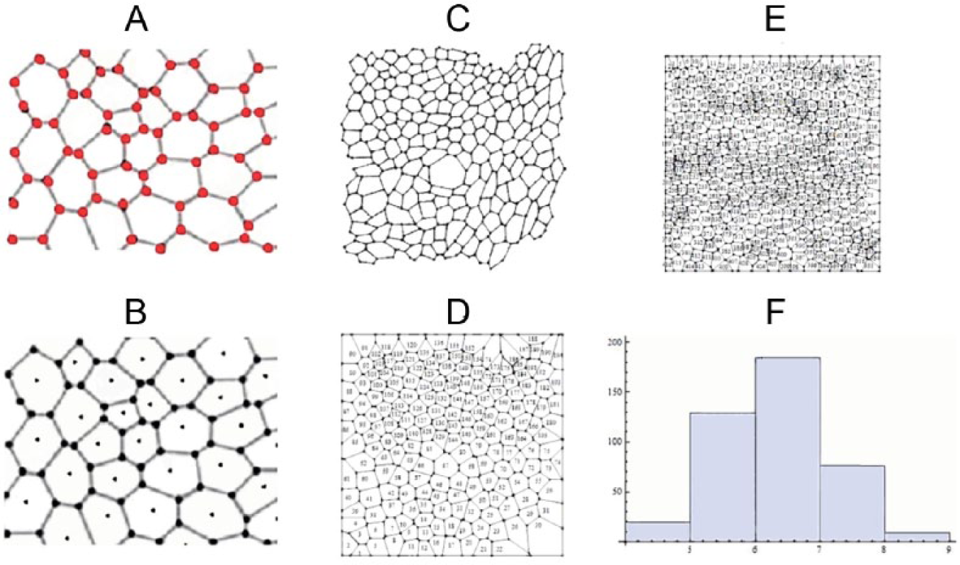
Epithelial topology lattice (set gamma 3). (A) Cell coordinates were extracted from edited images using the vertexes of polygons defining cells. (B) Those polygonal coordinates will define centroids to continue with the Voronoi treatment (n = 5). (C) Sample 0, n = 1, is extracted and edited from an open access image ⁷ to establish the polygonal coordinates of cells which have a regularity mean of global dispersion of 0.92. (D) Using the centroids established by the polygonal coordinates of sample 0, a Voronoi tessellation is obtained generating sample 1. (E) One of the remaining 4 samples obtained, generated by Voronoi treatment, is shown. (F) Universal epithelial frequency is shown which is equal for sample 0 and sample 1.

Figure 7.

Namibia circles lattice (set gamma 4). (A) One edited picture from an open access image of Namibia fairy circles (http://www.dailymail.co.uk/sciencetech/article-3160677/Will-mystery-Namibia-s-fairy-circles-solved-Stunning-images-reveal-astonishing-extent-baffling-grass-rings.html). The circles enclosed 3 Namibia fairy circles in a rough estimate. (B) The center of each circle defines the centroid to continue with the Voronoi treatment. (C) One of the 5 Voronoi tessellations is shown (n = 5).

Figure 8.

The Cairo tiling (set gamma 5). (A) Each vertex of the Cairo tiling defines a region around itself. (B) Eighty-six vertexes will define the centroids of each region. (C) One example of a Voronoi tessellation is generated (n = 1).

Spatial regions and random points as basic tools for developing Voronoi tessellation treatment

Once the lattice with particular spatial regions is defined, a random point is generated inside each cell to define localities in sets gamma 1 and 2. In contrast, centroids in sets 3, 4, and 5 are defined by vertexes of Cairo tiling, the centroids defined by polygonal coordinates, and the center of circles around “Fairy circles,” respectively. The next steps explain how the random and nonrandom points are generated on each lattice to make 5 sets $\gamma$ of polygons:

• Set gamma 1 (square lattice). In total, 100 pseudo-random points are generated inside 100 squares of magnitude 10 × 10, each in a proportional relation 1:1. The lattice is a square matrix of 10 × 10, defining a surface $R$ of 100 square units. In all, 50 Voronoi tessellations are generated using every sample of pseudo-random points, resulting in 50 sets gamma with 100 localities each (Figure 4).

• Set gamma 2 (the Cairo tiling random lattice). In total, 65 pseudo-random points are generated inside 65 regions whose centroids are the Cairo tiling vertexes. The vertexes are of 2 kinds: the vertex of those nodes with (1) 4 polygons as neighbors (16 vertexes) and those with (2) 3 polygons as neighbors (49 vertexes). The ratio to establish the random points is 8.5 units for nodes a and 11.41 for nodes b. These 2 magnitudes are defined regarding the condition that no 2 points are closer than a certain distance r and inscribed inside its own area. Fifty Voronoi tessellations are generated using every sample of pseudo-random points, giving 50 sets gamma of polygons with 65 localities each (Figure 5).

• Set gamma 3 (epithelial topology lattice; sample 0 and sample 1 correspond to this set). Five samples of epithelial topology images extracted from the web were edited to extract the centroids of cells. Also, we extract the number of cell neighbors of the original image ¹⁰ to provide the data for polygonal frequency. Using the centroids, we establish 5 Voronoi tessellations to define the localities, which were different in number for the 5 edited images. Sample 0 is a nonedited lattice using the coordinates as references to extract regularity data. Six sets gamma of polygons are generated as a result (Figure 6).

• Set gamma 4 (Namibia circles lattice). Five samples of Namibia fairy circles images extracted from the web were edited to extract the centroids of circles. Also, we extract the number of cell neighbors of the original image. Using the centroids, we establish 5 Voronoi tessellations to define the localities, which might be different in the number of these localities. Five sets gamma of polygons are generated as a result (Figure 7).

• Set gamma 5 (the Cairo tiling lattice; highly regular control). One Voronoi tessellation is generated using the vertexes of the Cairo tiling. The vertexes are of 3 kinds: the vertexes of those nodes with (1) 4 polygons as neighbors (16 vertexes) and those with (2) 3 polygons as neighbors (49 vertexes) and (3) those marking the borders of the image tiling (21 vertexes). One Voronoi tessellation is generated with 86 localities. One set gamma of polygons is generated as a result (Figure 8).

The 5 sets gamma of polygons that result from this methodology will constitute the material to measure eutacticity. Each polygon of every set gamma is the data source of coordinates to apply equation (3) which is $\epsilon$ parameter. The final number of sets gamma is 112: 50 from square lattice, 50 from the Cairo tiling random lattice, 6 from the epithelial topology lattice, 5 from Namibia circles lattice, and 1 from the Cairo tiling lattice. In addition, MGD (equation (2)) and GDG will be obtained from those coordinates. High spatial heterogeneity will be defined by low MGD and high GDG. A high MGD will imply low spatial heterogeneity or high regularity. Therefore, summation of polygonal eutactic values is a direct measure of MGD, and the standard deviation of this statistical parameter is GDG. The limits of eutactic values are 0.7 for low values and 1 for high eutactic values (equation (4)).

Results

To contrast to polygonal frequencies and regularity measures, we include Kolmogorov-Smirnov (KS) test to analyze the strength of polygonal distributions by themselves, accounting for regularity. We consider the UEF of polygons as a geometric standard and we analyze the statistical distances among polygonal distributions as a quantitative parameter using KS test. Our first hypothesis was a positive correlation between closeness among the distribution of UEF and polygonal distribution of samples (KS values) and the MGD value of samples. According to KS test, some samples can be very close to a UEF; even its regularity remains similar to the mean of a random sample (0.92; Figure 9A). The value of KS is inversely proportional to the distance between 2 statistical distributions. The KS is applied to visualize distribution distances between UEF and the Cairo tiling lattice or set gamma 5 (Figure 9B).

Figure 9.

Polygonal frequency is measured according to statistical distribution distances. Kolmogorov-Smirnov (KS) test is used to detect similarities between polygonal frequencies of sets gamma (blue line) with universal epithelial frequency (red line). (A) The KS distance for sample 0 and sample 1 with universal epithelial frequency is near 0.643 in both cases (blue line). Regularity mean of global dispersion (MGD) for sample 0 is 0.929 and regularity for sample 1 is 0.947. (B) The distance of polygonal distribution of highly regular control (blue line) from universal epithelial frequency (red line) is 0.00001206. The regularity MGD for the Cairo tiling (highly regular control) is 0.961.

In addition, spatial organization of biological patterns remains in gaps of high values for regularity MGD (Figure 10). Hence, our first hypothesis is rejected. In fact, the most notable result in this work is that all samples coming from biological systems, such as epithelial tissues and Namibia circles, have regularity values above 0.94 (Figure 10B). Sample 0 (from epithelial topology lattice or set gamma 4; Figure 10A) was considered a key reference to look at some important statistical differences in terms of regularity. That sample remains in a regularity value inside the limits of random samples (Figure 10A). Sample 0 was built using the polygon vertexes (locality $L_i$ ) of an epithelial sample without Voronoi treatment. This sample represents a set of polygons (N = 195) whose polygonal frequency is very similar to the UEF (KS distance is 0.64). However, this sample was not changed at all in terms of being modified by Voronoi tessellation treatment, and regularity is obtained using polygonal cell coordinates only. There were 2 samples derived from this original lattice, sample 0 and sample 1. Sample 1 (from epithelial topology lattice or set gamma 4; Figure 10B) was developed using the centroids derived from polygonal coordinates of each cell which were the points for the Voronoi tessellation treatment that will constitute the seeds for Voronoi construction that yields a new set of polygons. Regularity in sample 1 (from set gamma 3) increased to 0.947; this agrees with the results of Contreras-Figueroa et al. ¹⁷ As a conclusion, sample 0 and sample 1 have the same number of polygons, and their polygonal frequency is also very close to the UEF. Nevertheless, in terms of regularity, they are not the same; sample 0 is 0.929 and sample 1 is 0.947. In fact, there is no correlation between KS data and regularity of lattices of sets gamma in total data (r = 0.327). With these results, we conclude that spatial organization determining the nature of UEF is not just a fact regarding polygonal frequency; rather, it is related to area distribution inside shapes. Then, polygonal frequency of epithelial topology is only one of at least 2 possible conditions to establish a proper biological spatial organization inside global shapes. Polygonal frequency is only a partial condition determining proper biological spatial organization because a particular distribution of area inside polygons is also necessary. Finally, Figure 10B also shows samples 1 to 5 for set gamma 4 or Namibia circles lattice.

Figure 10.

(A) The range for regularity mean of global dispersion using eutactic average for each set gamma in random lattices remains 0.89 to 0.94, whereas (B) it is 0.94 to 0.968 for epithelium and Namibian fairy circles lattices.

According to our results, the MGD and GDG are not a random fact in lattices from sets gamma. The range for regularity MGD in random lattices remains 0.89 to 0.94 with n = 101 iterations (50 from set gamma 1 or square lattice, 50 from set gamma 2 or the Cairo tiling random lattice, and 1 for sample 0 from set gamma 4 or epithelial topology lattice; Figure 10A), whereas it is in the range of 0.94 to 0.968 values for epithelium (set gamma 4 or epithelial topology lattice; n = 5) and Namibian fairy circles (set gamma 5 or Namibia circles lattice; n = 5) lattices (Figure 10B). Also, the average of regularity in these last 10 different sets gamma (epithelial topology lattice and Namibia circles lattice) reflects the fact that there is a higher level for regularity in epithelium (0.955) and Namibian fairy circles (0.943), in contrast to random lattices (0.917 for set gamma 1 and 0.924 for set gamma 2; Figure 11A). However, the average of standard deviation is lower in epithelium (0.042) and Namibian fairy circles (0.039; Figure 11B) than in random lattices (0.0540 for square lattice, 0.0547 for the Cairo tiling random lattice). It is important to show that the highly regular lattice used as control, such as that emerging from set gamma 5 or the Cairo tiling lattice, is higher at both regularity and standard deviation values (Figure 11).

Figure 11.

(A) The average of total samples per group reflects the fact that there is a higher level for regularity in epithelium topology lattice (0.955 set gamma 4; n = 5) and Namibian circles lattice (0.943 set gamma 5; n = 5) in contrast to square lattice (0.917; n = 50) and the Cairo tiling random lattice (0.924; n = 50). (B) The average of standard deviation is lower in epithelium (0.042 set gamma 3) and Namibian fairy circles (0.039 set gamma 4) than in random lattices (0.0540, 0.0547 sets gamma 1 and 2). Highly regular lattices used as control, such as those emerging from the Cairo lattice (set gamma 5), are higher at both regularity (0.961) and standard deviation values (0.063).

The standard deviation decline is constant throughout sample data of biological architectures (Figure 12). Both epithelial samples and Namibian samples (sets gamma 3 and 4) show a decrease in standard deviation (right black arrow Figure 12) and an increase in regularity, in contrast to random samples from different lattices (sets gamma 1 and 2). However, the order of Cairo tiling pattern (set gamma 5) represents a control to show the closeness with higher regularity or low spatial heterogeneity. Nevertheless, this closeness was not reflected in a reduction in GDG (Figure 11B and right peak in Figure 12), and the polygonal distance with UEF is clear (Figure 9B).

Figure 12.

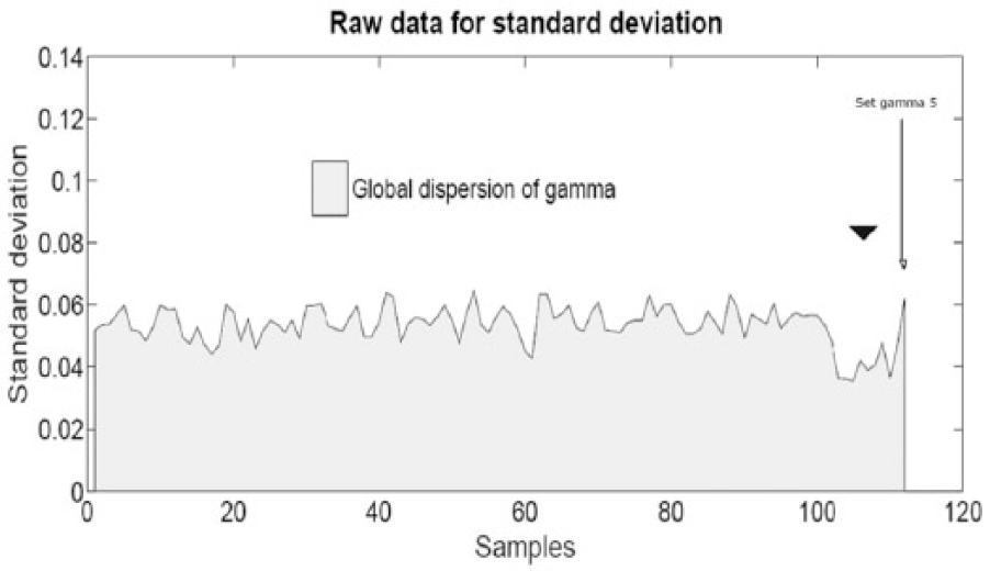
The standard deviation decline is constant throughout samples of biological architectures which can be visualized at right extreme. Sample 112 is a highly regular lattice used as control (Cairo tiling pattern). A draw guide to the eye is used to show the decline of sample (101-111) standard deviation and the increase of that value at the right side (arrow for sample 112 from set gamma 5).

Finally, the Kruskal-Wallis analysis for lattices reveals that there are some lower positive values for some ranks in random lattices (Figure 13A); every biological lattice falls over 1.86 (Figure 13B), which is a statistically high rank. The inclusion of the nonparametric test Kruskal-Wallis is motivated because the distribution of eutactic values is a non-normal distribution. We conclude that there were significant statistical differences in terms of spatial distributions between biological architectures and nonbiological ones.

Figure 13.

(A) The Kruskal-Wallis analysis for lattices reveals that there are some lower positive values for some ranks in random lattices, and (B) every biological lattice falls over 1.862. Sample 0 falls in the rank of 0.337 above the control mark limiting random lattices from negative rank values.

Discussion

In summary, our results suggest that according to our first proposed parameter (MGD value), spatial organizations of those 2 case studies analyzed are demarcated by being in a position among spatial order and disorder (eutactic values below 0.968 and above 0.94; Figure 10B). In contrast, random lattices are limited to be in a different lower rank of spatial organization (0.89 and 0.94; Figure 10A). However, the value of spatial organization for regularity control (0.961) is higher than that of biological samples (0.943 and 0.955; Figure 11). In addition, the difference in GDG (second proposed parameter) between the Cairo tiling and biological tiling was not expected because highly regular lattices should reduce its degrees of freedom (Figure 11B). These results need to be evaluated with some other highly ordered lattices to find a decisive conclusion. Our method proves the information about geometric constructions of 2 biological architectures limited to a zone of particular spatial organization. We conclude that this particular spatial organization is an important condition to start defining the potentiality of geometric constraints in a very complex morphospace. The nature of shapes in terms of statistical organization can be turned into an extended theoretical and practical device ready to understand the limits of biological organization. Nontrivial associations can result from apparently distinct shapes that at the deepest point share the same spatial organizations. In addition, this measure would have practical implementations because the geometric values of the constricted zone can be translated in some other parametric devices ready to provide information about biological behaviors such as resilience, robustness, and evolvability. It is important to continue with the implementation of the test to detect the scope of quantification of spatial organization in defining the very deep essence of shapes and patterns in nature.